Article

Mathematical Modeling of Two Interacting Populations’ Dynamics of Onchocerciasis Disease Spread with Nonlinear Incidence Functions

by
Kabiru Michael Adeyemo
1,
Umar Muhammad Adam
2,
Adejimi Adeniji
3 and
Kayode Oshinubi
4,*
1
Department of Mathematics, Hallmark University, Ijebu-Itele 122101, Nigeria
2
Department of Mathematics, Federal University, Dutse 720222, Nigeria
3
Department of Mathematics and Statistics, Tshwane University of Technology, Pretoria 0183, South Africa
4
School of Informatics, Computing and Cyber Systems, Northern Arizona University, Flagstaff, AZ 86011, USA
*
Author to whom correspondence should be addressed.
Mathematics 2024, 12(2), 222; https://doi.org/10.3390/math12020222
Submission received: 30 October 2023 / Revised: 30 December 2023 / Accepted: 5 January 2024 / Published: 9 January 2024

Abstract

:
The transmission dynamics of onchocerciasis in two interacting populations are examined using a deterministic compartmental model with nonlinear incidence functions. The model undergoes qualitative analysis to examine how it behaves near disease-free equilibrium (DFE) and endemic equilibrium. Using the Lyapunov function, it is demonstrated that the DFE is globally stable when the threshold parameter R 0 1 is taken into account. When R 0 > 1 , it suffices to show globally how asymptotically stable the endemic equilibrium is and its existence. We conduct the bifurcation analysis by looking at the possibility of the model’s equilibria coexisting at R 0 < 1 but near R 0 = 1 using the Center Manifold Theory. We use the sensitivity analysis method to understand how some parameters influence the R 0 , hence the transmission and mitigation of the disease dynamics. Furthermore, we simulate the model developed numerically to understand the population dynamics. The outcome presented in this article offers valuable understanding of the transmission dynamics of onchocerciasis, specifically in the context of two populations that interact with each other, considering the presence of nonlinear incidence.

1. Introduction

Commonly Known as “river blindness” [1], onchocerciasis is a neglected tropical illness that is brought on by the filarial nematode Onchocerca volvulus, a parasitic worm [2].
Onchocerciasis [3] is transferred via the repeated bites of black flies, specifically those belonging to the Simulium species. It is commonly found and widespread in that region [4]. Understanding the spread of this disease and how it can be mitigated is still a subject of discussion among researchers, public health experts, and modelers because it still puts a given population at risk. Researchers have investigated the interaction between infectious disease and species coexistence [5], and the impact of Lotka-Volterra on infectious disease [6]. It is imperative to know that there are other models that are variants of predator-prey models, such as Holling-Tanner model [7] with an infected prey. Refs. [8,9] consider the effect of disease with respect to treatment, the influence of education awareness vector control, and the age group with the informative period discrimination of serology; however, the incidence was not the point of focus.
An optimal control of the disease can be achieved by applying mitigation strategies of personal protection using treated bed-net wearing, permethrin-treated cloths, surgical care for humans with body deformation and impaired vision, education campaigns, and the use of insecticides [10]. Ivermectin can be delivered consistently either annually or biannually in Nigeria, which would effectively lower the risk of illness. In addition, public health management measures are required to reduce the risk of infectious human-blackfly contact, which can result in infections with onchocerciasis and blindness [11]. In South Sudan, the incidence of epilepsy linked to onchocerciasis is predicted to drop significantly by over 50% during the first five years of yearly mass medication administration with at least 70% coverage. The frequency of onchocerciasis-associated epilepsy can be halved in approximately 10 years, but the reduction is slower when vector control at a high efficacy level is the only tactic used. Better outcomes were obtained in avoiding new instances of onchocerciasis-associated epilepsy when vector control was implemented concurrently with mass medication administration, and its efficacy levels were raised [11]. Ref. [8], looks into the consequences of four control measures: mass drug treatment with ivermectin, public health education, larviciding, and trapping. It also gives a mathematical transmission model of onchocerciasis dynamics. According to the model, the best way to stop onchocerciasis from spreading is to combine all four therapies. Along with simulation and numerical data, the research also deduces the basic reproduction rate in the presence of the interventions. Overall, the study’s conclusions point to the need for a thorough strategy to control onchocerciasis in order to effectively treat the illness. Mass Ivermectin administration was disrupted by the COVID-19 pandemic, which had an impact on the short-term trends and the progress of onchceriacis elimination by 2030 [12]. The most impacted programs will be those with shorter histories of mass drug administration and those in environments with significant pre-intervention endemicity. Reducing coverage is not as successful as reducing the influence of COVID-19 on mass medication administration or as biannual mass drug administration is. There should be little impact on programs that had already moved to biennial mass medication administration [6]. Significant progress has been made in reducing the burden of this parasitic disease over the past few decades. In 1995, nearly 19 million individuals were estimated to be afflicted with onchocerciasis. However, promisingly, projections indicate that by 2025, the prevalence of this disease is expected to have declined substantially, with only approximately four million cases remaining. This marked reduction in the number of affected individuals reflects the impact of various control measures and interventions. The majority are anticipated to reside in hypoendemic areas that are not the primary focus of mass drug administration efforts, underscoring the complex dynamics of disease control strategies and regional variations in disease prevalence [13].
Researchers have conducted various studies exploring potential methods to mitigate the transmission of the disease. In one study [14], researchers utilized the skin snip survey in West Africa to assess the impact of mitigating black flies through larviciding. In another study [15], the authors employed a microsimulation model to determine the optimal duration for combining annual ivermectin treatment [16] and vector mitigation in an onchocerciasis mitigation program in West Africa, aiming to identify effective strategies for disease control. Additionally, in the studies [8,17], the researchers employed computer simulation models to investigate onchocerciasis prevention. While one study examined the effects of four strategies on control of the disease’s spread, the other concentrated on macrofilaricide, which targets adult worms.
Furthermore, a simple mathematical framework is presented in [18] to analyze host age-profiles of infection prevalence in northern Cameroon. The mathematical approach used in the study in northern Cameroon is likely to account for the age-dependent characteristics and concerns in disease transmission. The supplied model, on the other hand, presents a more complete representation, with age-specific compartments for humans and explicit vector dynamics. Furthermore, the given model integrates recovery and mortality rates for both human and vector populations, allowing for a thorough examination of age-group interactions and the impact of mortality on disease dynamics. The framework chosen relies on the individual research aims and the level of detail sought in capturing onchocerciasis transmission dynamics. A deterministic framework with estimated parameter values from the Mexican onchocerciasis control program is presented in [19] to assess the construction of models for onchocerciasis utilizing a variety of methodologies.
The recent COVID-19 pandemic has been extensively studied by many researchers and it is important to mention an article from which we employ some of the ideas presented since one of the improvements we added in this research is to consider nonlinear incidence functions. To capture the dynamics of the COVID-19 pandemic, lag parameters should be included to account for before an exposed person could become infected. Therefore, it was investigated in [1] employing the SEIR epidemic model, which incorporated a time delay and convex incidence.
The onchocerciasis transmission model focuses on vector-borne transmission, human-vector interactions, and age structure, taking into account the disease’s peculiar dynamics. The SEIR model for COVID-19, on the other hand, focuses on human-to-human transmission, asymptomatic spread, immunity dynamics, vaccination, and the influence of public health measures. The assumptions of each model are customised to the specific characteristics of the respective diseases, emphasising the importance of disease-specific modelling methodologies in informing effective public health interventions.
Having reviewed some papers in the research area considered in this article, the novelty of our work lies in the introduction of two interacting populations and adding nonlinear incidence functions to the mathematical model we developed, which is an extension of our previous work in [20] in which we presented the local stability analysis of the model. In this work, we investigate the dynamics of onchocerciasis transmission using nonlinear incidence functions. There are four distinct populations among the human population, which represent different states or groups within the population, while three compartments make up the vector population, representing different stages or categories of the vector population. The global asymptotic behavior in disease-free (disease-free equilibrium as DFE), endemic equilibria and the bifurcation analysis was shown and examined. Finally, we present some quantitative analysis. The remainder of the paper is structured as follows: Section 2 provides a description of the model and theorems on positivity of solutions; Section 3 focuses on the demonstration of global stability theorems; and Section 4 conducts a bifurcation analysis of the model. In Section 5, we present some quantitative analysis and make some concluding remarks in Section 6.

2. Model Description

There are two populations considered for interaction purposes; black flies and humans. The human population is compartmentalized into four: the susceptible human; S h , the exposed human; E h , the infectious human; I h and the recovered human; R h . The black fly population is compartmentalized into three: the susceptible-vector; S v , the exposed-vector; E v and the infectious-vector. The total numbers of humans and vectors at a specific time t, are represented as; N = S h ( t ) + E h ( t ) + I h ( t ) + R h ( t ) and V = S v ( t ) + E v ( t ) + I v ( t ) . It is assumed that spread of onchocerciasis in susceptible hosts occurs only through contact with an infectious vector. By assumption, the susceptible vector would become infectious after the contact with a host that is infected during a blood meal. It is expected that the study population is sizable to be modeled deterministically. The dynamics of onchocerciasis epidemics are described by the system of nonlinear ODEs with non-negative initial conditions that follow.
d S h ( t , x i ) d t = Ψ h ( x i ) i = 0 L δ λ h ( x i ) S h ( t , x i ) I v ( t ) 1 + ν h ( x i ) I v ( t ) μ h ( x i ) S h + w ( x i ) R h ( t , x i ) d E h ( t , x i ) d t = i = 0 L δ λ h ( x i ) S h ( t , x i ) I v ( t ) 1 + ν h ( x i ) I v ( t ) ( α h ( x i ) + μ h ( x i ) ) E h ( t , x i ) d I h ( t , x i ) d t = i = 0 L α h ( x i ) E h ( r ( x i ) + γ h ( x i ) + μ h ( x i ) ) I h ( t , x i ) d R h ( t , x i ) d t = i = 0 L r ( x i ) I h ( μ h ( x i ) + w ( x i ) ) R h ( t , x i ) d S v d t = Ψ v δ λ v ( x i ) S v ( t ) I h ( x i , t ) 1 + ν v I h ( x i , t ) μ v S v ( t ) d E v d t = δ λ v ( x i ) S v ( t ) I h ( x i , t ) 1 + ν v I h ( x i , t ) ( α v + μ v ) E v ( t ) d I v d t = α v E v ( t ) ( μ v + γ v ) I v ( t ) }
with initial conditions:
S h ( 0 , x i ) = S 0 h ( x i ) , E h ( 0 , x i ) = E 0 h ( x i ) , I h ( 0 , x i ) = I 0 h ( x i ) , R h ( 0 , x i ) = R 0 h ( x i ) , S v ( 0 ) = S 0 v , E v ( 0 ) = E 0 v , I v ( 0 ) = I 0 v
Model assumptions
The following assumptions form the basis of the compartmental model’s formulation:
  • Every member of the human population is initially vulnerable to the illness, which means they could get it.
  • Infected sensitive individuals in the human population go into the exposed state, where they are not contagious.
  • After being exposed, the affected persons develop into infectious individuals, who can spread the illness to other people.
  • Infected people can die naturally or from the disease, but if not, they return to be cured of their human illness through treatment.
  • After individuals recover from the infection, they become susceptible to the disease once more, implying that they can potentially contract it in future.
  • Since all black flies are initially prone to the sickness, it follows that they have the potential to contract the infection.
  • When susceptible black flies become infected, they transition into the exposed state, where they are still not able to infect humans with the disease.
  • The black flies in the exposed state subsequently progress to becoming infectious, where they can transmit the disease to humans.
  • There is no distinct recovered class for the population of black flies since the infected black flies stay infectious for the whole of their lives.
In Table 1 and Table 2, we present the description of population state variables and parameters of the onchocerciasis model respectively.

Existence and Positivity of the Model Solutions

We address the dynamics of the positive, bounded, and invariant solutions to the proposed model of system (1) in this section. Both for humans and black flies, this explains population dynamics. Under the above criteria, the system discussed here is relevant to biology.
Ω = ( S h ( t , x i ) , E h ( t , x i ) , I h ( t , x i ) , R h ( t , x i ) ) R + 4 : N h i = 0 L Ψ h ( x i ) μ h ( x i ) , ( S v ( t ) , E v ( t ) , I v ( t ) ) R + 3 : N v Ψ v μ v ,
These results provided show that the governing model in system (1) is well-posed in a region that is feasible Ω as
Ω = Ω h × Ω v R 4 × R 3
Theorem 1. 
Within the domain Ω, there is a contained and bounded solution set
S h ( t , x i ) , E h ( t , x i ) , I h ( t , x i ) , R h ( t , x i ) , S v ( t ) , E v ( t ) , I v ( t ) .
Proof. 
If N h = S h ( t , x i ) + E h ( t , x i ) + I h ( t , x i ) + R h ( t , x i ) represents the total size of the human population, then N v = S v ( t ) + E v ( t ) + I v ( t ) represents the total number of black fly population. Model (1) gives us the following
d N h ( t , x i ) d t Ψ h ( x i ) i = 0 L μ h ( x i ) N h ( t , x i )
and
d N v d t Ψ v μ v N v
It follows from (3) and (4) that
N h ( t , x i ) Ψ h ( x i ) μ h ( x i ) [ 1 e 1 μ h ( x i ) t ] + N h ( 0 , x i ) e μ h ( x i ) t ]
and
N v Ψ v μ v [ 1 e μ v t ] + N v ( 0 ) e μ v t
Taking the lim s u p as t gives N h Ψ h ( x i ) μ h ( x i ) and N v Ψ v μ v . This analysis demonstrates that all solutions pertaining to the human population are limited to the solution set Ω h , while all solutions related to the black fly population are confined within the solution set Ω v . It is enough to say that Ω is positive invariant because N h ( t , x i ) i = 0 L Ψ h ( x i ) μ h ( x i ) whenever N h ( 0 , x i ) Ψ h ( x i ) μ h ( x i ) and N v ( t ) Ψ v μ v if N v ( 0 ) Ψ v μ v , Therefore, the model (1) solution set exists and is given as Ω = Ω h × Ω v R + 4 × R + 3
To complete the analysis, it is crucial to demonstrate that the solutions of system (1) are non-negative within the solution set Ω for any time t > 0 . This is particularly important as the variables in the system represent the populations of humans and black flies, which are inherently non-negative.
Positive invariance assures that populations such as susceptible, exposed, infectious, and recovered individuals stay positive across time, given non-negative initial conditions. This mathematical condition is critical for the model’s validity since it corresponds to the physical fact that populations cannot have negative counts. Positive invariance ensures that the model’s predictions are realistic and that the dynamics of onchocerciasis transmission depicted by the model remain epidemiologically relevant throughout the simulation.
Theorem 2. 
Given non-negative initial conditions within the solution set Ω, the solutions S h ( t , x i ) , E h ( t , x i ) , I h ( t , x i ) , R h ( t , x i ) , S v ( t ) , E v ( t ) , and I v ( t ) of model (1) will stay non-negative within Ω for all t > 0 . This guarantees that over the course of the whole time period, the populations of black flies and humans, which are represented by these variables, will always remain non-negative.
Proof. 
Initial conditions are given as, S 0 h ( x i ) , E 0 h ( x i ) , I 0 h ( x i ) , R 0 h ( x i ) , S 0 v , E 0 v , I 0 v , are positive and from (1),
d S h ( t , x i ) d t + i = 0 L b λ h ( x i ) I v ( t ) 1 + ν h ( x i ) I v ( t ) + μ h ( x i ) S h ( t , x i ) 0 ,
by integrating (5), we have
i = 0 L S h ( t , x i ) i = 0 L S 0 h ( x i ) e x p 0 t b λ h ( x i ) I v ( η ) 1 + ν h ( x i ) I v ( η ) d η + μ h ( x i ) t 0 ,
this implies ∀ t > 0 and a R + , we have
S h ( t , x i ) i = 0 L S 0 h ( x i ) e x p 0 t b λ h ( x i ) I v ( η ) 1 + ν h ( x i ) I v ( η ) d η + μ h ( x i ) t 0 .
We have, S h ( t , x i ) > 0 for any arbitrary x i . In the same vein
d E h ( t , x i ) d t + i = 0 L ( ( α h ( x i ) + μ h ( x i ) ) ) E h ( t , x i ) 0
so that
d d t i = 0 L E h ( t , ( x i ) ) e x p ( α h ( x i ) + μ h ( x i ) t ) 0
By means of Integration (7), we have ∀ t > 0 and for all a R + , that
E h ( t , a ) i = 0 L E 0 h ( x i ) e x p ( α h ( x i ) + μ h ( x i ) ) t
Hence, E h ( t , x i ) > 0 for any arbitrary x i Also we have
d I h ( t , x i ) d t i = 0 L ( r ( x i ) + γ h ( x i ) + μ h ( x i ) ) I h ( t )
so that
d d t I h ( t ) e x p ( r ( x i ) + γ h ( x i ) + μ h ( x i ) ) t 0
Similarly, (8) becomes
I h ( t , a ) i = 0 L I 0 h e x p ( r ( x i ) + γ h ( x i ) + μ h ( x i ) ) t > 0 for all t > 0 for all a R +
Therefore, for each arbitrary x i , I h ( t , x i ) > 0 . From (1), we obtain
d R h ( t , x i ) d t + i = 0 L ( μ h ( x i ) + w ( x i ) ) R h ( t , x i ) 0 ,
and integrating (9), we have, t > 0 and a R , that
R h ( t , a ) i = 0 L R 0 h ( x i ) e x p ( ( μ h ( x i ) + w ( x i ) ) t ) > 0
Hence, R h ( t , x i ) > 0 for any arbitrary x i . In same manner, we obtain
d S v d t + i = 0 L b λ v I h ( t ) ) 1 + ν v I h ( t ) + μ v S v ( t ) 0
so that
d d t S v ( t ) e x p 0 t b λ v I h ( η ) ) 1 + ν v I h ( η ) d ( η ) + μ v t 0
Integrating (9), we have
S v ( t ) S 0 v e x p 0 t b λ v I h ( η ) ) 1 + ν v I h ( η ) d ( η ) + μ v t > 0 t > 0
Also we have
E v ( α v + μ v ) E v ( t ) ,
which on integration gives
E v ( t ) E v ( 0 ) e x p ( α v + μ v ) t > 0 t > 0 ,
we obtain,
I v + ( μ v + γ v ) I v ( t ) ,
to have
I v ( t ) I v ( 0 ) e x p ( μ v + γ v ) t > 0 , t > 0
The theorem on the existence of solutions establishes the mathematical well-posedness of a model describing onchocerciasis transmission. Ensuring meaningful predictions, the model includes a derivative, d E h ( t , x i ) d t , representing the rate of change of exposed humans over time. The interplay between terms involving α h (per capita rate of progression), μ h (human mortality rate), I h (rate of transition to infectious state), and R h (number of humans recovered) is crucial. α h dictates the speed of transition from exposed to infectious states, μ h counters this progression through mortality, I h contributes to the increase in infectious individuals, and R h represents the number of recovered individuals. Together, it is important to note that these components enlighten the dynamics of the movement from exposed to infectious states in the human population, ensuring the model’s flow in describing the transmission of onchocerciasis.

3. Analysis of DFE and Endemic Equilibrium

3.1. Disease-Free Equilibrium (DFE)

The DFE points represent steady state which depicts the lack of infection in the populations of black flies and humans. This means that onchocerciasis is not present within the individuals at these points. The DFE, E 0 , of the model (1) depicts that S * ( x i ) h 0 , E h * ( x i ) = I h * = 0 ( x i ) = R h * ( x i ) = 0 , S v * 0 , E v = I v = 0 substituting into (1), we obtain S * ( x i ) h = Ψ h ( x i ) μ h ( x i ) and S v * = Ψ v μ v . Consequently we obtain E 0 as
E 0 = Ψ h ( x i ) μ h ( x i ) , 0 , 0 , 0 , Ψ v μ v , 0 , 0
In the analysis of the models with a presence of the infectious disease, a fundamental concept is the basic reproduction number ( R 0 ), this indicates the level of incidence which requires the degree of response to be either immediate. It plays a crucial role in determining whether a disease will fade out or remain within the population. A next generation matrix is introduced to obtain the R 0 of the system (1) and is represented as
R 0 = R h R v
where R h = i = 0 L δ α h ( x i ) λ h ( x i ) Ψ h ( x i ) μ h ( x i ) ( α h ( x i ) + μ h ( x i ) ) ( r ( x i ) + γ h ( x i ) + μ h ( x i ) ) and R v = δ α v λ v Ψ v μ v ( α v + μ v ) ( γ v + μ v ) . The R 0 for onchocerciasis is instrumental in determining whether the disease will fade out or remain within population. R h represents the average number of humans that are infected by a single infectious black fly over its expected period of contagiousness, assuming all human populations are susceptible. On the other hand, R v represents the average number of black flies that are infected by a single human during the contagious duration, considering completely susceptible black fly inhabitants. These values provide information on the disease’s potential for persistence and propagation.

3.2. Global Stability Analysis

Here, we explore the global asymptotic stability of the DFE and EE for the special case with no loss of immunity acquired by the recovered individuals. We use the concept of Lyapunov functions to analyze the global stability.

3.3. Global Stability of Disease-Free Equilibrium

The following result establishes the global asymptotic behavior of system (1) around E 0 which is determined by the basic reproduction number R 0 .
Theorem 3. 
The disease-free equilibrium (12) of model (1) is globally asymptotically stable in Ω whenever R 0 1
Proof. 
Consider the linear Lyapunov function of the form
M = c 1 E h ( t , x i ) + c 2 I h ( t , x i ) + c 3 E v ( t ) + c 4 I v ( t )
where
c 1 = α b ( x i ) μ v ( x i + μ h ( x i ) ) ( r ( x i ) + γ h ( x i ) + μ h ( x i ) )
c 1 = 1 μ b ( r ( x i ) + γ h ( x i ) + μ h ( x i ) )
c 3 = 1 δ λ v Ψ v
c 4 = α v + μ v δ γ v α v Ψ v
In what follows, the time derivative of M along the solutions of the model (1) yields
M ˙ = α h ( x i ) μ v ( α h ( x i ) + μ h ( x i ) ) ( r ( x i ) + γ h ( x i ) + μ h ( x i ) ) × i = 0 L δ λ h ( x i ) S h ( t , x i ) I v 1 + ν h ( x i ) I v ( α h ( x i ) + μ h ( x i ) ) E h ( t , x i ) + 1 = 0 L α h ( x i ) E h ( t , x i ) ( r ( x i ) + γ h ( x i ) + μ h ( x i ) ) I h ( t , x i ) μ v ( r ( x i ) + γ h ( x i ) + μ h ( x i ) ) + 1 δ λ v Ψ v δ λ v S v I h ( t , x i ) 1 + ν v I h ( t , x i ) ( α v + μ v ) E v + α v + μ v δ λ v α v Ψ v [ α v E v ( μ v + γ v ) I v ]
By simplifying further, we have
M ˙ = i = 0 L δ α h ( x i ) λ h ( x i ) S h ( t , x i ) I v μ v ( α h ( x i ) + μ h ( x i ) ) ( r ( x i ) + γ h ( x i ) + μ h ( x i ) ) ( 1 + ν h ( x i ) I v ) I h ( t , x i ) μ v + S v I h ( t , x i ) Ψ v ( 1 + ν v I h ( t , x i ) ) ( α v + μ v ) ( μ v + γ v ) I v δ λ v α v Ψ v i = 0 δ α h ( x i ) λ h ( x i ) Ψ h ( x i ) I v μ h μ v ( α ( x i ) + μ h ( x i ) ) ( r ( x i ) + γ h ( x i ) + μ h ( x i ) ) ( α v + μ v ) ( μ v + γ v ) I v δ λ v Ψ v = ( α v + μ v ) ( μ v + γ v ) δ λ v α v Ψ v [ R 0 1 ] I v
Therefore M ˙ 0 for R 0 0 if and only if I v = 0 . Further, one sees that
( S h ( t , x i ) , E h ( t , x i ) , I h ( t , x i ) , R h ( t , x i ) , S v ( t ) , E v ( t ) ) Ψ h ( x i ) μ h ( x i ) , 0 , 0 , 0 , Ψ v μ v , 0
as t since I v 0 as t . Consequently, the largest compact invariant set in { ( S h ( t , x i ) , E h ( t , x i ) , I h ( t , x i ) , R h ( t , x i ) , S v ( t ) , E v ( t ) , I v ( t ) ) Ω : M ˙ = 0 } is the singleton { E 0 } and by LaSalle’s invariance principle [7], E 0 is globally asymptotically stable in Ω . □
The global asymptotic stability analysis of the endemic equilibrium is considered next for the special case with ω ( x i ) = 0 . The disease-present (endemic) equilibrium of the model (1) is referred to as the steady-state solution where at least one of the infected compartments is nonzero. Let the arbitrary endemic equilibrium of the model (1) be represented by E e = ( S h * * ( x i ) , E h * * ( x i ) , I h * * ( x i ) , R h * * ( x i ) , S m * * , E m * * , I m * * ) In order to do this, nonlinear Lyapunov function is used of Goh-Volterra type [6,15].
Theorem 4. 
The unique endemic equilibrium, E e , of the model (1) is globally asymptotically stable if R 0 > 1 .
Proof. 
Let R 0 > 1 so that there exists a unique endemic equilibrium and consider the nonlinear Lyapunov function defined by
M = S h ( t , x i ) S h * * ( x i ) S h * * ( x i ) ln S h ( t , x i ) S h * * ( x i ) + E h ( t , x i ) E h * * ( x i ) E h * * ( x i ) ln E h ( t , x i ) E h * * ( x i ) + i = 0 L α h ( x i ) + μ h ( x i ) α h ( x i ) I h ( t , x i ) I h * * ( x i ) I h * * ( x i ) ln I h ( t , x i ) I h * * ( x i ) + S v S v * * S v * * ln S v S v * * + E v E v * * E v * * ln E v E v * * + α v + μ v α v I v I v * * I v * * ln I v I v * *
With Lyapunov time-derivative given as
M ˙ = S ˙ h ( t , x i ) S h * * ( x i ) S h ( x i ) S ˙ h ( t , x i ) + E ˙ h ( t , x i ) E h * * ( x i ) E h ( x i ) E ˙ h ( t , x i ) + i = 0 L α h ( x i ) + μ h ( x i ) α h ( x i ) I ˙ h ( t , x i ) I h * * ( x i ) I h ( x i ) I ˙ h ( t , x i ) + S ˙ v S v * * S v S ˙ v + E ˙ v E v * * E v E ˙ v + α v + μ v α m I ˙ v I v * * I v I ˙ v
Using equations of the model (1) in (16) we obtain
M ˙ = Ψ h ( x i ) i = 0 L δ λ h ( x i ) S h ( t , x i ) I v 1 + ν h ( x i ) I v μ h ( x i ) S h ( t , x i ) i = 0 L S h * * ( x i ) S h ( t , x i ) Ψ h ( x i ) δ λ h ( x i ) S h ( t , x i ) I v 1 + ν h ( x i ) I v μ h ( x i ) S h ( t , x i ) + i = 0 L δ λ h ( x i ) S h ( t , x i ) I v 1 + ν h ( x i ) I v + [ α h + μ h ] E h ( t , x i ) i = 0 L E h * * ( x i ) E h ( t , x i ) δ λ h ( x i ) S h ( t , x i ) I v 1 + ν h ( x i ) I v + [ α h + μ h ] E h ( t , x i ) + i = 0 L α h ( x i ) + μ h ( x i ) α h ( x i ) × ( α h ( x i ) E h ( t , x i ) [ r ( x i ) + μ h ( x i ) + γ h ( x i ) ] ) I h ( t , x i ) i = 0 L I h * * ( x i ) ( α h ( x i ) + μ h ( x i ) ) I h ( t , x i ) α h ( x i ) × ( α h ( x i ) E h ( t , x i ) [ r ( x i ) + μ h ( x i ) + γ h ( x i ) ] ) I h ( t , x i ) + Ψ v δ λ v S v I h ( t , x i ) 1 + ν v I h ( t , x i ) μ v S v S v * * S v Ψ v δ λ v S v I h ( t , x i ) 1 + ν v I h ( t , x i ) μ v S v + δ λ v S v I h ( t , x i ) 1 + ν v I h ( t , x i ) + [ α v + μ v ] E v E v * * E h ( t , x i ) δ λ h ( x i ) S h ( t , x i ) I v 1 + ν h ( x i ) I v + [ α h + μ h ] E v + α v + μ v α v α v E v [ μ v + γ v ] I v I v * * I v ( α v E v [ μ v + α v ] I v )
Let g ( I v ) = I v 1 + ν h ( x i ) I v and g ( I h ) = I h ( t , x i ) 1 + ν v ( x i ) I h ( t , x i ) then simplifying M ˙ gives
M ˙ = i = 0 L Ψ h ( x i ) 1 S h * * ( x i ) S h ( t , x i ) i = 0 L μ h ( x i ) S h ( t , x i ) 1 S h * * ( x i ) S h ( t , x i ) + i = 0 L δ λ h ( x i ) S h * * ( x i ) g ( I v ) i = 0 L E h * * ( x i ) δ λ h ( x i ) S h ( t , x i ) g ( I v ) E h ( t , x i ) + i = 0 L ( α h ( x i ) + μ h ( x i ) ) E h * * ( x i ) i = 0 L ( α h ( x i ) + μ h ( x i ) ) α h ( x i ) ( r ( x i ) + μ h ( x i ) γ h ( x i ) ) I h ( t , x i ) i = 0 L ( α h ( x i ) + μ h ( x i ) ) I h * * ( x i ) E h ( t , x i ) I h ( t , x i ) + i = 0 L α h ( x i ) + μ h ( x i ) α h ( x i ) ( r ( x i ) + μ h ( x i ) + γ h ( x i ) ) I h * * ( x i ) + Ψ v 1 S v * * S v μ v S v 1 S v * * S v + δ λ v S v * * ( x i ) g ( I h ) E v * * δ λ v S v g ( I h ) E v + ( α v + μ v ) E v * * ( α v + μ v ) ( μ v + γ v ) I v α v ( α v + μ v ) I v * * E v I v + ( α v + μ v ) ( μ v + γ v ) I v α v
At the endemic equilibrium E e , we get from model (1) that
Ψ h ( x i ) = i = 0 L δ λ h ( x i ) S h * * ( x i ) g ( I v * * ) + i = 0 L μ h ( x i ) S h * * ( x i ) α h ( x i ) + μ h ( x i ) = i = 0 L δ λ h ( x i ) S h * * g ( I v * * ) E h * * ( x i ) r ( x i ) + μ h ( x i ) + γ h ( x i ) = i = 0 L α h ( x i ) E h * * ( x i ) I h * * ( x i ) Ψ v = δ λ v S v * * g ( I h * * ) + μ v S m * * α v + μ v = δ λ v S m * * g ( I h * * ) E v * * μ v + γ v = α v E v * * I v * *
Using (16) in (18), we have
M ˙ = i = 0 L μ h ( x i ) S h * * 2 S h * * ( x i ) S h ( t , x i ) S h ( t , x i ) S h * * ( x i ) + i = 0 L δ λ h ( x i ) S h * * ( x i ) g ( I v * * ) i = 0 L δ λ h ( x i ) ( S h * * ) 2 g ( I v * * ) S h ( x i ) + δ λ h ( x i ) S h * * ( x i ) g ( I v ) i = 0 L E h * * ( x i ) δ λ h ( x i ) S h ( t , x i ) g ( I v ) E h ( t , x i ) + δ λ h ( x i ) S h * * ( x i ) g ( I v ) i = 0 L δ λ h ( x i ) S h * * ( x i ) I h ( t , x i ) g ( I v * * ) I h * * ( x i ) i = 0 L δ λ h ( x i ) I h * * ( x i ) E h ( t , x i ) g ( I v * * ) E h * * ( x i ) I h ( t , x i ) + i = 0 L δ λ h ( x i ) S h * * g ( I v * * ) + μ v S v * * 2 S v * * S v S v S v * * δ λ v S v * * g ( I h * * ) δ λ v ( S v * * ) 2 g ( I h * * ) S v + δ λ v S v * * g ( I h ) E v * * δ λ v S v g ( I h ) E v + δ λ v S v * * g ( I h ) δ λ v S v * * I v g ( I h * * ) I v * * δ λ v I v * * E v g ( I h * * ) E v * * I v + δ λ v S v * * g ( I h * * )
Simplifying further, we have
M ˙ = i = 0 L μ h ( x i ) S h * * 2 S h * * ( x i ) S h ( t , x i ) S h ( t , x i ) S h * * ( x i ) + i = 0 L δ λ h ( x i ) S h * * g ( I v * * ) × 4 S h * * ( x i ) S h ( t , x i ) E h * * ( x i ) S h ( t , x i ) g ( I v ) E h ( t , x i ) S h * * g ( I v * * ) I h * * ( x i ) E h ( t , x i ) I h ( t , x i ) E h * * ( x i ) I h ( t , x i ) g ( I v * * ) I h * * ( x i ) g ( I v ) + i = 0 L δ λ h ( x i ) S h * * g ( I v * * ) δ λ ( x i ) S h * * ( x i ) I h ( t , x i ) g ( I v * * ) I h * * ( x i ) + i = 0 L δ λ h ( x i ) S h * * ( x i ) I h ( t , x i ) g 2 ( I v * * ) I h * * ( x i ) f ( I v ) δ λ h ( x i ) S h * * g ( I v * * ) + μ v S v * * 2 S v * * S v S v S v * * + δ λ v S v * * g ( I h * * ) × 4 S v * * S v E v * * S h ( t , x i ) g ( I h ) E v S v * * g ( I h * * ) I v * * E v I v E v * * I v g ( I h * * ) I v * * g ( I h ) + δ λ v S v * * g ( I h * * ) δ λ v S v * * I v g ( I h * * ) I v * * + δ λ v S v * * I v g 2 ( I h * * ) I v * * g ( I h ) δ λ v S v * * g ( I h * * )
Further simplification yields
M ˙ = M ˙ 1 M ˙ 2 δ λ h ( x i ) S h * * ( x i ) g ( I v * * ) 1 g ( I v ) g ( I v * * ) + I h ( t , x i ) I h * * ( x i ) + I h ( t , x i ) g ( I v * * ) I h * * ( x i ) g ( I v ) M ˙ 3 M ˙ 4 δ λ v S v * * g ( I h * * ) 1 g ( I h ) g ( I h * * ) + I v I v * * + I v g ( I h * * ) I v * * g ( I h )
where
M 1 = i = 0 L μ h ( x i ) S h * * ( x i ) S h * * ( x i ) S h ( t , x i ) + S h ( t , x i ) S h * * ( x i ) 2 , M 2 = i = 0 L δ λ h ( x i ) S h * * ( x i ) g ( I v ) × S h * * ( x i ) S h ( t , x i ) + E h * * ( x i ) S h ( t , x i ) g ( I v ) E h ( t , x i ) S h * * g ( I v * * ) + I h * * ( x i ) E h ( t , x i ) I h ( t , x i ) E h * * ( x i ) + I h ( t , x i ) g ( I v * * ) I h * * ( x i ) g ( I v ) 4 M 3 = μ v S v * * S v * * S v + S v S v * * 2 M 4 = δ λ v S * * S v * * S v + E v * * S v ( t , x i ) g ( I h ) E v S v * * g ( I h * * ) + I v * * E v I v E v * + I v g ( I h * * ) I v * * g ( I h ) 4
Using arithmetic mean and geometric mean inequality and whenever g ( I h * * ) g ( I h ) = I v * * I v , it follows (22) that M 0 with M = 0 if and only if S h ( t , x i ) = S h * * ( x i ) , E h ( t , x i ) = E h * * ( x i ) , S h ( t , x i ) = S h * * ( x i ) , I h ( t , x i ) = I h * * ( x i ) , S m ( t ) = S m * * , E m ( t ) = E m * * , I m ( t ) = I m * * .
This further implies
R h ( t , x i ) r ( x i ) I h * * μ h = R h * * .
Since
( S h ( t , x i ) , E h ( t , x i ) , I h ( t , x i ) , S m ( t ) , E m ( t ) , I m ( t ) ) ,
tends to
( S h * * ( x i ) , E h * * ( x i ) , I h * * * * ( x i ) , S m * * , E m * * , I m * * ) .
as t .
Therefore, by LaSalle’s principle, the largest compact invariant subset of the set where M is the the endemic equilibrium point, E e .
Thus, every solution in Ω approaches E e for R 0 > 1 and E e is globally asymptotically stable. □

4. Bifurcation Analysis

Bifurcation analysis refers to the mathematical investigation of qualitative changes in the behavior of a dynamical system as a parameter crosses a critical value known as a bifurcation point. This analysis aims to understand the various types of bifurcations and their impact on the system’s dynamics, such as changes in stability, the emergence of new solutions, or the appearance of periodic or chaotic behavior. Bifurcation analysis plays a vital part in understanding the behavior of complex dynamical systems and can provide insights into their underlying mechanisms.
Theorem 5 
([21]). Consider the following general system of ordinary differential equation with a parameter φ:
d y d t = f ( y , φ ) , f : R n × R R a n d f C ( R n × R )
where 0 is an equilibrium point of the system (that is, f ( 0 , φ ) 0 for all φ) and we have the following assumptions:
  • A = D y f ( 0 , 0 ) = D y f ( 0 , 0 ) , is the linearization matrix of the system in Theorem 5 around the equilibrium 0 where φ evaluated at 0. A’s simple eigenvalue is zero, while its other eigenvalues have real components that are negative;
  • The right eigenvector κ of Matrix A is non-negative, while the left eigenvector η corresponds to the zero eigenvalue.
Let f k represent k t h component of f and
m = k , i , j = 1 n η k κ i κ j 2 f k y i y j ( 0 , 0 ) ,
n = i , j = 1 n η k κ i 2 f k y i φ ( 0 , 0 )
The signs of m and n dictate the system’s local dynamics entirely around 0.
  • m > 0 , n > 0 . When φ < 0 with | φ | < < 1 , 0 is locally stable asymptotically and ∃ an unstable equilibrium that is positive; when 0 < φ < < 1 , 0 is unstable and ∃ a negative, locally stable asymptotically equilibrium;
  • m < 0 , n < 0 . When φ < 0 with | φ | < < 1 , 0 is unstable; when 0 < φ < < 1, 0 is locally stable asymptotically, and ∃ an unstable equilibrium that is positive;
  • m > 0 , n < 0 . When φ < 0 with | φ | < < 1 , 0 is unstable, and ∃ a locally asymptotically stable equilibrium that is negative; when 0 < φ < < 1 , 0 is stable, and a unstable equilibrium appears that is positive;
  • 0 transforms φ ’s stability from stable to unstable when it goes from negative to positive. As a result, a negatively unstable equilibrium turns positive and asymptotically stable locally. In particular, if m > 0 and n > 0 , then there exists a backward bifurcation.
To illustrate the potential for the model’s (1) equilibria to coexist at R 0 < 1 but near R 0 = 0 , the Center Manifold Theory described by [21] Let the onchocerciasis model (1) be written in the vector form
d ρ d t = Σ ( ρ )
where ρ = ρ 1 , ρ 2 , ρ 3 , ρ 4 , ρ 5 , ρ 6 , ρ 7 T and Σ = σ 1 , σ 2 , σ 3 , σ 4 , σ 5 , σ 6 , σ 7 T so that S h ( t ; x i ) = ρ 1 ; E h ( t ; x i ) = ρ 2 ; I h ( t ; x i ) = ρ 3 ; R h ( t ; x i ) = ρ 4 ; S v ( t ) = ρ 5 ; E v ( t ) = ρ 6 ; and I v ( t ) = ρ 7 : Then model (1) becomes
d ρ 1 d t = Ψ h ( x i ) δ λ h ( x i ) ρ 1 ρ 7 1 + ν h ( x i ) ρ 7 μ h ( x i ) ρ 1 + ω ( x i ) ρ 4 = σ 1 d ρ 2 d t = δ λ h ( x i ) ρ 1 ρ 7 1 + ν h ( x i ) ρ 7 ( α h ( x i ) + μ h ( x i ) ) ρ 2 = σ 2 d ρ 3 d t = α h ρ 2 ( r ( x i ) + μ h ( x i ) + γ h ( x i ) ) ρ 3 = σ 3 d ρ 4 d t = r ( x i ) ρ 3 ( μ ( x i ) + ω h ( x i ) ) ρ 4 = σ 4 d ρ 5 d t = Ψ v δ λ v ( x i ) ρ 5 ρ 3 1 + ν h ( x i ) ρ 3 μ v ( x i ) ρ 5 = σ 5 d ρ 6 d t = δ λ v ( x i ) ρ 5 ρ 3 1 + ν h ( x i ) ρ 3 ( α v + μ v ) ρ 6 = σ 6 d ρ 7 d t = α v ( μ v + γ v ) x 7 = σ 7 }
Let λ h ( x i ) be a bifurcation parameter such that λ h ( x i ) = λ h * ( x i ) when R 0 = 1 . Then
λ h * ( x i ) = i = 0 L μ h ( x i ) μ v ( α h ( x i ) + μ h ( x i ) ) ( r ( x i ) + μ ( x i ) h + γ h ( x i ) ) ( μ v + γ ) ( α v + μ v ) δ 2 α h ( x i ) Ψ h ( x i ) α v λ v Ψ v
The linearization matrix M ( E 0 ; λ h * ( x i ) ) of the model (1), evaluated at the DFE E 0 and the bifurcation parameter λ h * ( x i ) , is given
M ( E 0 ; λ h * ( x i ) ) = μ h ( x i ) 0 0 ω ( x i ) 0 0 A 0 B 0 0 0 0 C 0 α h ( x i ) D 0 0 0 0 0 0 r ( x i ) E 0 0 0 0 0 G 0 μ v 0 0 0 0 K 0 0 L 0 0 0 0 0 0 α v M
where A = i 0 L δ λ h * ( x i ) Ψ h ( x i ) μ h ( x i ) , B = ( α h ( x i ) + μ h ( x i ) ) , C = i 0 L δ λ h * ( x i ) Ψ h ( x i ) μ h ( x i ) , D = ( r ( x i ) + γ h ( x i ) + μ h ( x i ) ) , E = ( μ h ( x i ) + ω ( x i ) ) , G = δ λ v Ψ v μ v , K = δ λ v Ψ v μ v , L = ( α v + μ v ) , M = ( μ v + γ v ) .
The eigenvalues of M ( E 0 , λ h ( x i ) ) can be acquired by the characteristic equation’s solution.
( ξ + μ h ( x i ) ) ( ξ + μ h ) ( ξ + μ h ( x i ) + ω ( x i ) ) P 1 ( ξ ) = 0 ,
where P 1 ( ξ ) is a polynomial of degree four. Consequently, M ( E 0 , λ * ( x i ) ) possesses a simple zero eigenvalue; the remaining eigenvalues are real and negative. Let us represent the eigenvector corresponding on right to this zero eigenvalue as κ = κ 1 , κ 2 , κ 3 , κ 4 , κ 5 , κ 6 , κ 7 7 so that M ( E 0 , λ h * ( x i ) ) κ = 0 . Then we have
μ h ( x i ) κ 1 + ω ( x i ) κ 4 + A κ 7 = 0 B κ 2 A κ 7 = 0 α h ( x i ) κ 2 + D κ 3 = 0 r ( x i ) κ 3 + E κ 4 = 0 G κ 3 μ v κ 5 = 0 G κ 3 + L κ 6 = 0 α v κ 6 + M κ 7 = 0
From (25), the components of the right eigenvector κ are given by
κ 1 = U κ 6 κ 2 = ( r ( x i ) + γ h ( x i ) + μ h ( x i ) ) ( α v + μ v ) μ v κ 6 δ λ v Ψ v α ( x i ) κ 3 = ( α v + μ v ) μ v κ 6 δ λ v Ψ v κ 4 = r ( x i ) ( α v + μ v ) μ v κ 6 δ λ v Ψ v ( μ h ( x i ) + ω ( x i ) ) κ 5 = ( α v + μ v ) κ 6 μ v κ 6 = 1 T 1 κ 7 = α v κ 6 μ v + γ v
U = i = 0 L ( α v + μ v ) μ v δ λ v Ψ v α h ( x i ) μ h ( x i ) ( μ h ( x i ) + ω ( x i ) ) ( r ( x i ) α h ( x i ) ( α h ( x i ) + μ h ( x i ) + ω ( x i ) ) + ( γ h ( x i ) + μ h ( x i ) ) ( r ( x i ) + γ h ( x i ) + μ h ( x i ) ) ( μ h ( x i ) + ω ( x i ) )
and
T 1 = α v [ ( α v + μ v ) ( μ v + γ v ) ( r ( x i ) + μ h ( x i ) + γ h ( x i ) + μ v ( α h ( x i ) + μ h ( x i ) ) ) + i = 0 L ( α h ( x i ) + μ h ( x i ) ) ( r ( x i ) + μ h ( x i ) + γ h ( x i ) ) ( 2 μ v + γ v + α v ) ]
Further, M ( E 0 , λ * ( x i ) ) has a left eigenvector, η = ( η 1 , η 2 , η 3 , η 4 , η 5 , η 6 , η 7 ) , associated with the zero eigenvalue, which can be obtained from η M ( E 0 , λ * ( x i ) ) = 0 as follows: = −(αh(ai) + µh(ai))(r(ai) + µh(ai) + δh(ai))(αm + µm)(µm + δm)
η 1 = 0 η 2 = δ λ v α v α h ( x i ) Ψ v η 7 ( α h ( x i ) + μ h ( x i ) ) ( r ( x i ) + μ h ( x i ) + γ h ( x i ) ) ( α v + μ v ) η 3 = δ λ v α v Ψ v η 7 ( r ( x i ) + μ h ( x i ) + γ h ( x i ) ) ( α v + μ v ) η 4 = 0 η 5 = 0 η 6 = α v η 7 α v + μ v η 7 = ( α h ( x i ) + μ h ( a i ) ) ( r ( x i ) + μ h ( x i ) + γ h ( x i ) ) ( α v + γ v )
We see from the system in Theorem 5 that all the second-order partial derivatives at E 0 and λ ( x i ) are zero except the following:
2 f 1 y 1 y 7 = 2 f 1 y 7 y 1 = δ λ h * ( x i ) ,
2 f 2 y 1 y 7 = 2 f 2 y 7 y 1 = δ λ h * ( x i ) ,
2 f 5 y 3 y 5 = 2 f 5 y 5 y 3 = δ λ v , 2 f 6 y 3 y 5 = 2 f 6 y 5 y 3 = δ λ v
2 f 1 d y 7 2 = i = 0 L 2 δ λ h ( x i ) ν h ( x i ) Ψ h ( x i ) μ h ( x i ) , 2 f 2 d y 7 2 = i = 0 L 2 δ λ h ( x i ) ν h ( x i ) Ψ h ( x i ) μ h ( x i )
2 f 5 y 3 2 = 2 δ λ v Ψ v μ v , 2 f 6 y 3 2 = 2 δ λ v Ψ v μ v
tegether with
2 f 1 7 h ( x i ) = δ Ψ h ( x i ) μ h ( x i )
and
2 f 2 7 h ( x i ) = b Ψ h ( x i ) μ h ( x i )
If we let the bifurcation coefficients m and n of Theorem 5 be m 1 and n 1 respectively, it then follows from the above partial derivatives that
m 1 = i , j , k = 1 7 η k κ i κ j 2 f k y i y j ( E 0 , λ h * ( x i ) ) = 2 η 1 κ 1 κ 7 2 f 1 y 1 y 7 + η 1 κ 7 2 2 f 1 2 y j + 2 η 2 κ 1 κ 7 2 f 2 y 1 y 7 + η 2 κ 7 2 f 2 y 7 2 + 2 η 5 κ 3 κ 5 f 5 y 3 y 5 + η 5 κ 3 2 2 f 5 y 3 2 + 2 η 6 κ 3 κ 5 f 6 y 3 y 5 + η 6 κ 3 2 2 f 6 2 y 3
Substituting the appropriate right eigenvector (26), the left eigenvector (29) and the second-order partial derivatives obtained earlier into m 1 yields
m 1 = i = 0 L δ 2 λ h * ( x i ) λ v α v 2 α h ( x i ) Ψ v η 7 κ 6 2 U ( α h ( x i ) + μ h ( x i ) ) ( r ( x i ) + μ h ( x i ) + γ h ) ( α v + μ v ) ( μ v + γ v ) + i = 0 L δ λ v α v 2 α h ( x i ) Ψ v η 7 κ 6 2 ( α h ( x i ) + μ h ( x i ) ) ( r ( x i ) + μ h ( x i ) + γ h ( x i ) ) ( α v + μ v ) ( μ v + γ v ) 2 × 2 δ λ h * ( x i ) ν h ( x i ) Ψ h ( x i ) μ h ( x i ) 2 α v ( α v + μ v ) η 7 κ 6 2 Ψ v α v μ v ( α v + μ v ) ν v η 7 κ 6 2 δ λ v Ψ v
Similarly, we obtain
n 1 = k , i = 0 7 η k κ i 2 f k y i λ h ( E 0 , λ h * ( x i ) ) = 2 η 1 κ 7 2 f 1 y 7 λ h + 2 η 2 κ 7 2 f 2 y 7 λ h ( x i ) = i = 0 L 2 δ 2 α h ( x i ) α v 2 λ v Ψ v Ψ h ( x i ) η 7 κ 6 ( μ v + γ v ) ( α h ( x i ) μ h ( x i ) ) ( r ( x i ) + μ h ( x i ) + γ h ( x i ) ( α v + μ v ) μ h ( x i ) )
The signs of m 1 and n 1 are important in determining the direction of bifurcation at R = 1 [21] One sees that m 1 > 0 and n 1 > 0 and by item (iv) of Theorem 5, the model (1) has the ability of exhibiting a backward bifurcation characteristics. Thus, we have the following result:
Theorem 6. 
The onchocerciasis model given by (1) undergoes a phenomenon of backward bifurcation at E 0 and R 0 = 1 .
Figure 1 demonstrates that when the basic reproduction number R 0 grows, the vector force of infection changes qualitatively. This shift could suggest a shift in disease transmission patterns. When R 0 exceeds a crucial threshold, the force of infection among vectors may suddenly increase or shift. This could indicate a tipping point in the disease’s ability to spread within the population as labeled at different points on the diagram in Figure 1 showing when the DFE is globally stable at R 0 < 1 and unstable, and also when the unique endemic equilibrium is globally stable R 0 > 1 .

5. Quantitative Analysis

5.1. Simulation of Numerical Analysis

The numerical simulation of the model we developed in this paper was implemented using Python algorithm to obtain the dynamical behavior of the model population states. We used the following initial conditions: S h ( 0 , x i ) = 9000 , E h ( 0 , x i ) = 800 , I h ( 0 , x i ) = 10 , R h ( 0 , x i ) = 50 , S v ( 0 ) = 800 , E v ( 0 ) = 20 , I v ( 0 ) = 50 . We chose the time period of 10 weeks for our simulation. The parameters used for the simulation can be found in Table 2. We varied some of these parameters, while some were estimated and taken from the literature.
We provide a numerical approach for understanding transmission and varying the parameters to see how each compartment reacts when these parameters are changed. To accomplish this, we use the Runge-Kutta technique [22], which is a well-known and successful method for solving initial-value problems in differential equations. Because of its high precision and computational complexity level, the fourth order of the Runge-Kutta approach is utilized to create high-order accurate numerical methods for solving most infectious disease differential equations.
We consider the model (1) with its initial conditions, this is represented as:
y m = g 1 ( t , y 1 , y 2 , , y n ) ; y j ( t 0 ) = y 0 , j = 1 , 2 , 3 . , n
the y i s depicts the model (1) compartments. In providing solutions for the model, we use the RKF approach in two orders (order four and order five), such that the algorithm is implemented in distinct iteration phases. The fourth-order method has five phases and the fifth-order approach has six stages, and the mathematical representation is presented as follows in Equation (34):
v 1 = h f i ( t , y 1 , x 2 , , y n ) , v 2 = h f i ( t + 1 4 h , y 1 + 1 4 v 1 , y 2 + 1 4 v 1 , , y n + 1 4 v 1 ) , v 3 = h f i ( t + 3 8 h , y 1 + 3 32 v 1 + 9 32 v 2 , y 2 + 3 32 v 1 + 9 32 v 2 , , y n + 3 32 v 1 + 9 32 v 2 ) , v 4 = h f i ( t + 12 13 h , y 1 + 1932 2197 v 1 7200 2197 v 2 + 7296 2197 v 3 , y 2 + 1932 2197 v 1 7200 2197 v 2 + 7296 2197 v 3 , y n + 1932 2197 v 1 7200 2197 v 2 + 7296 2197 v 3 ) , v 5 = h f i ( t + h , y 1 + 439 216 v 1 8 v 2 + 3680 513 v 3 845 4104 v 4 , y 2 + 439 216 v 1 8 k 2 + 3680 513 v 3 845 4104 v 4 , y n + 439 216 v 1 8 v 2 + 3680 513 v 3 845 4104 v 4 ) , v 6 = h f i ( t + h , y 1 8 27 v 1 + 2 v 2 3544 2565 v 3 + 1859 4104 v 4 11 40 v 5 , y 2 8 27 v 1 + 2 v 2 3544 2565 v 3 + 1859 4104 v 4 11 40 v 5 y n 8 27 v 1 + 2 v 2 3544 2565 v 3 + 1859 4104 v 4 11 40 v 5 ) ,
As a result, it is considered the standard Runge-Kutta approach.The simulation is carried out investigating the population of each compartment against time, which is measured in weeks.
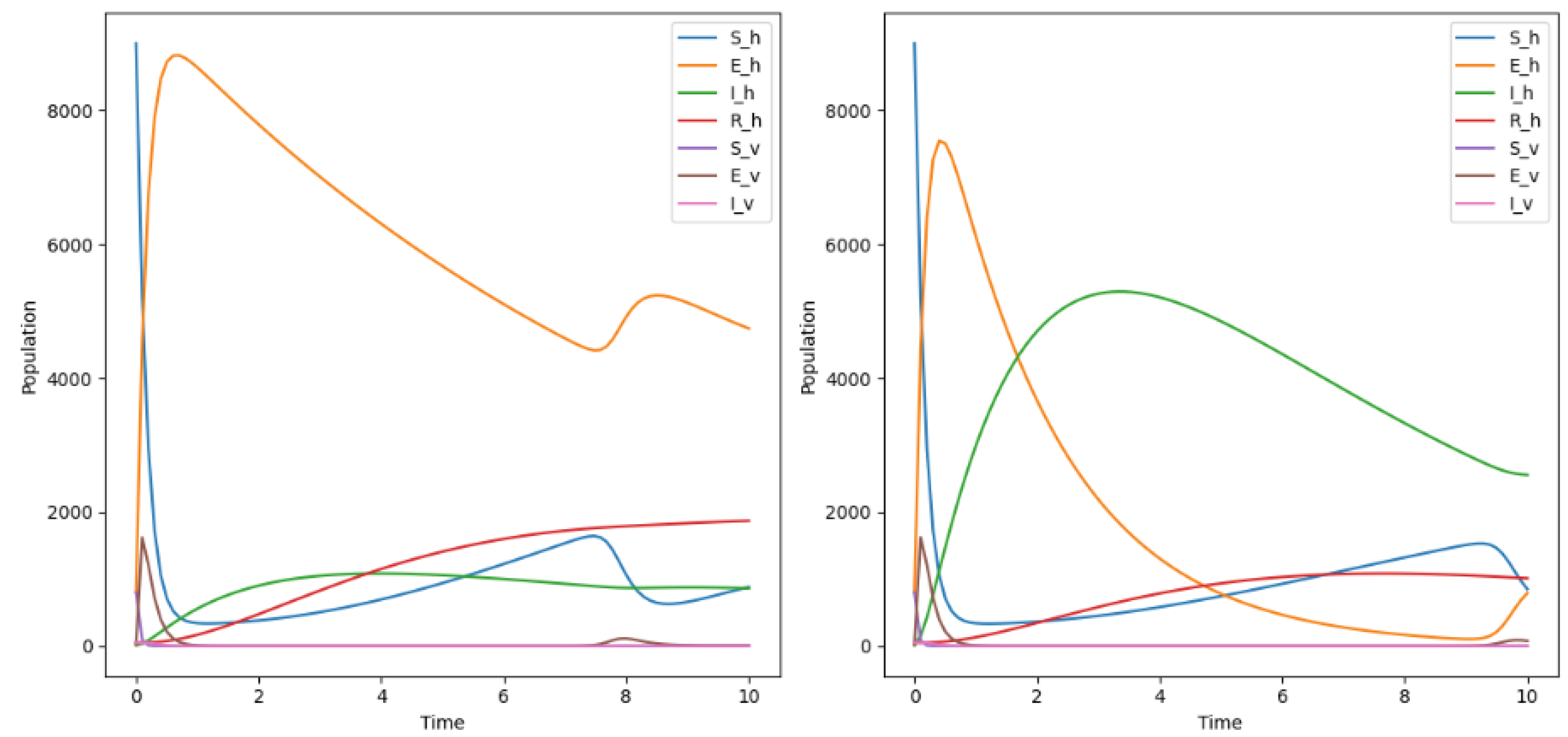
Figure 2 depicts the dynamics of our model and captures the first peak of the disease spread after almost twenty days of infected humans. We observe that very few black flies are exposed and infected which signifies the rapid decline in the population state varieties, noting that we have a lot of humans susceptible to the disease. Our simulation result is able to capture dynamics of the disease in the human and vector populations showing a significant in the exposed class in humans and vectors by extension infectious state if they rapidly progress to the population state.
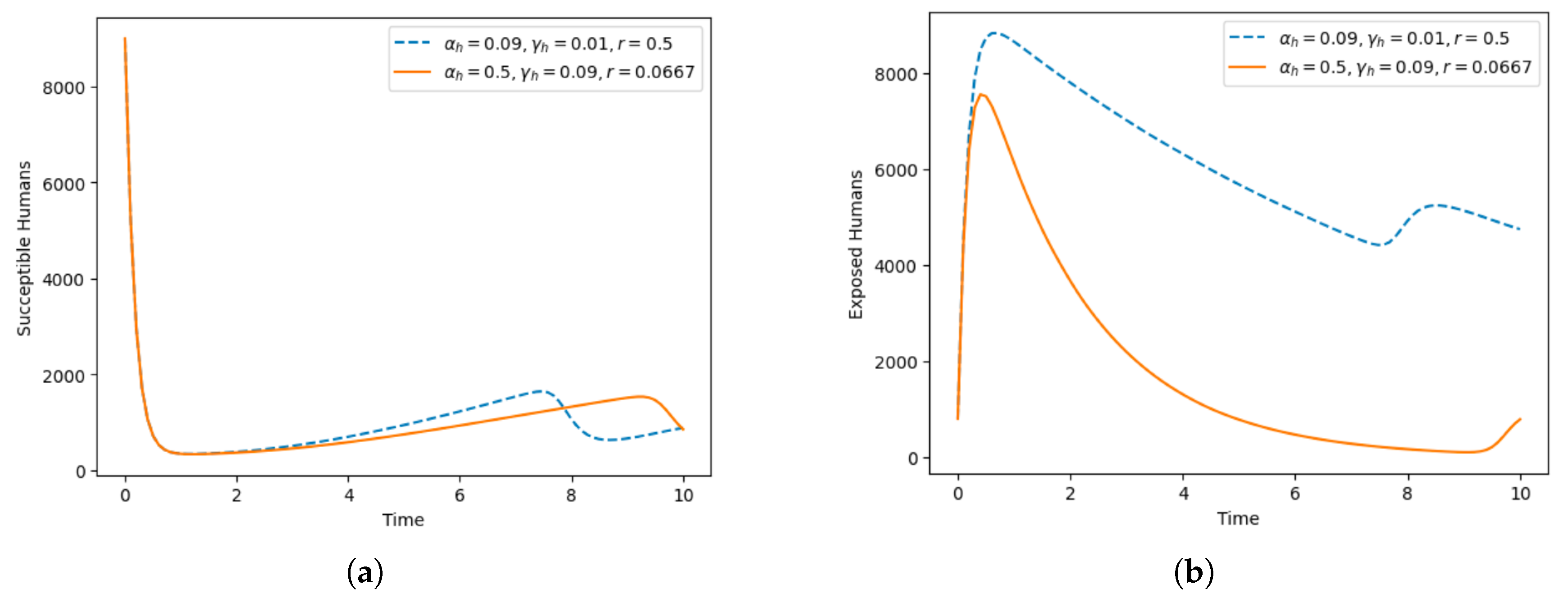
In the implementation of the numerical technique to foster understanding of each compartments, we provided Figure 3 and Figure 4. Looking at Figure 3a, this considers the susceptible population of humans against time measured in weeks. Varying the parameters of α h , γ h , and r which denote the progression of human from exposed to infectious state, mortality rate, and rate at which infected individual move to recovered state respectively, it can be inferred that the lower the infection rate, the more susceptible population is free of the Onchocerciasis disease. Figure 3b explain the dynamic attitude of the exposed compartment when the individual from the susceptible compartment become exposed to the onchocerciasis disease, higher rate of exposure of the individual to the infected disease will result in much spikes within one week one week but this can be mitigated if the exposure of individuals from the disease can be reduced, meaning the lower the exposure then the slower the movement rate. Observing Figure 4a,b which is the infected and recovered population, we can see that the exposure of the human population to the disease, increase with massive high spike. The higher the value of α h and γ h of the human, the higher the population of the infected individuals and the lower their recovery rate; what this means is that more people are affected with the Onchocerciasis disease. Looking at the recovered population, we can see that increase in the movement (r) to the recovery compartment (i.e the movement from the infected compartment to the recovered compartment) and lower values for the α h and γ h , begins to the reduce the spike of the infected people and give a gradual spike in the recovered people who were once infected.

5.2. Sensitivity Analysis

5.2.1. Sensitivity Analysis of Basic Reproduction Number, R h

The sensitivity analysis is obtained by taking a partial derivative of the basic reproduction number with respect to each of its parameters. It identifies the parameters that most influence the disease’s transmission and assesses the potential effects of parameter uncertainty on the dynamics of the epidemic. With regard to its parameters, let us assume Q, the sensitivity index of the fundamental reproduction number, R h , is as follows:
S Q R h = R h Q · Q R h
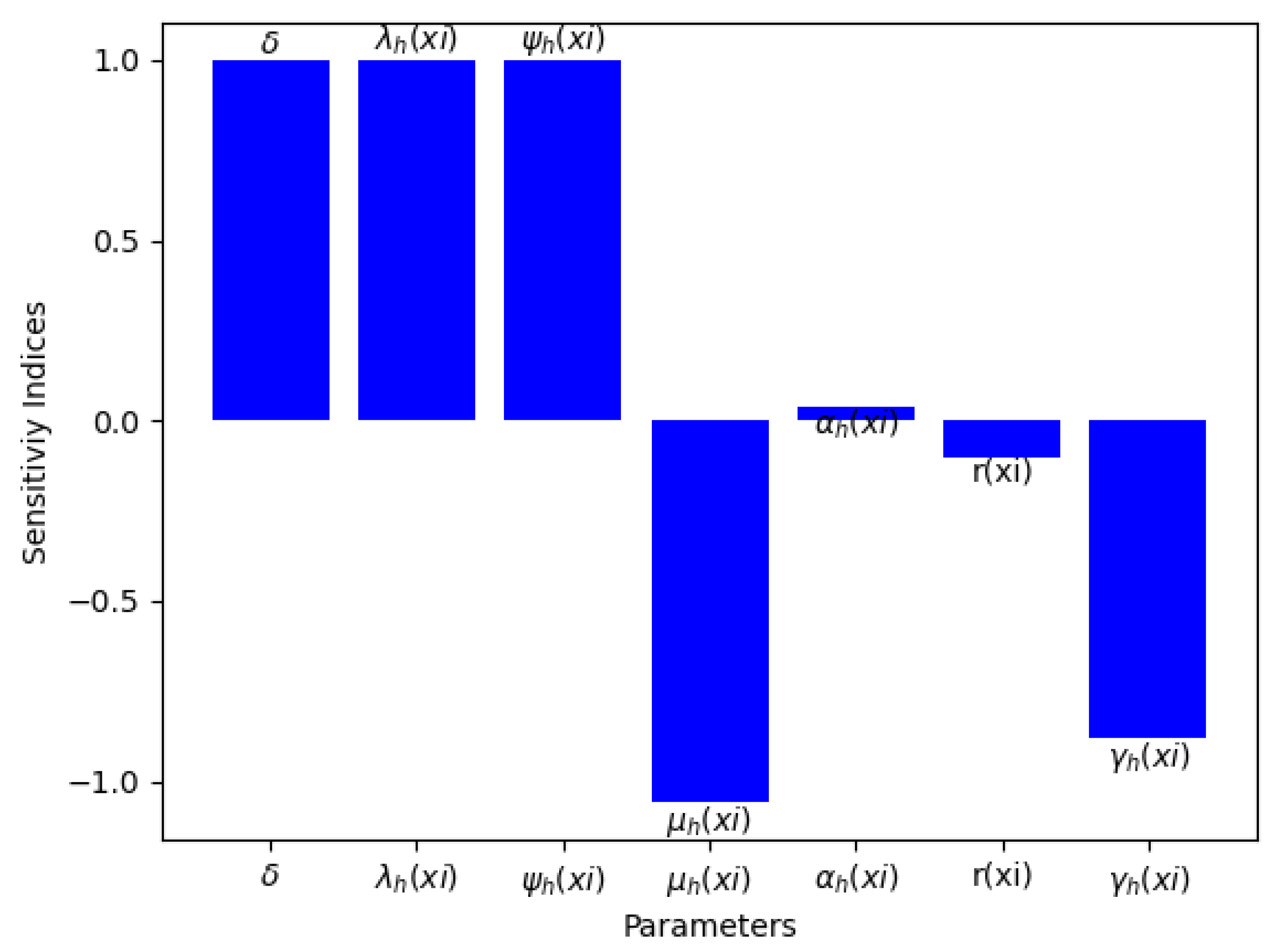
Table 3 shows that three of the sensitivity indices are negative and four are positive. The basic reproduction number’s sensitivity analysis reveals a direct relationship between R h and the vector’s biting rate, the recruitment term of susceptible humans, and the likelihood that an infectious vector bite will cause a human to contract the disease. In contrast, other parameters have an inverse relationship with R h . Table 3 and Figure 5 present the sensitivity indices as they relate to R h .
What can be deduced from the sensitivity analysis of R h is that if the rate at which the bite of an infectious vector is reduced by means of prevention, the threshold parameter R h will decrease, which means the spread of the disease will be curtailed.

5.2.2. Sensitivity Analysis of Basic Reproduction Number, R v

With regard to parameter P, the sensitivity index of the basic reproduction number, R v , is as follows:
S P R v = R v P · P R v
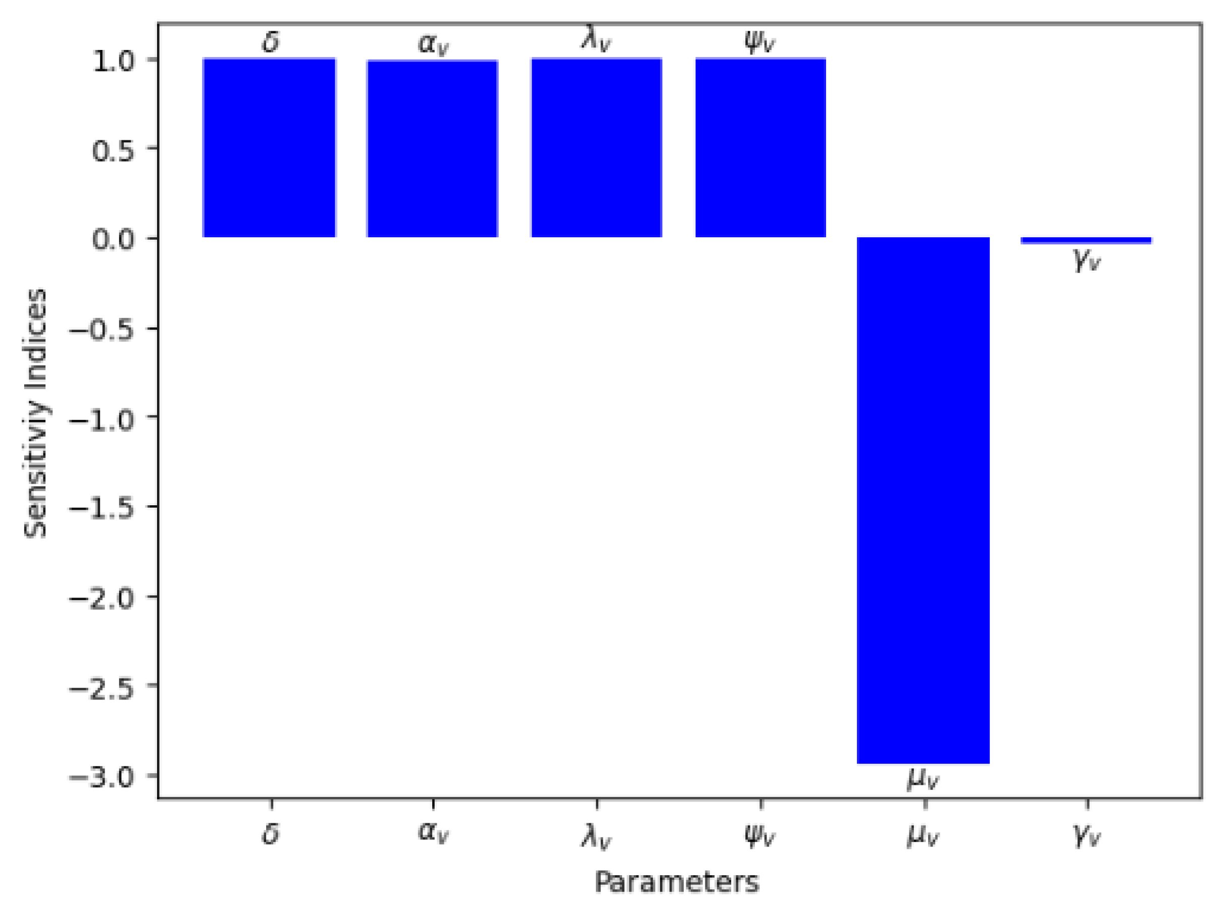
Table 4 displays that four of the sensitivity indices are positive and the other two are negative. The basic reproduction number, R v , underwent sensitivity analysis. The results indicate that there is a direct correlation between R v and the vector’s biting rate, susceptible vectors’ recruitment term, the vectors’ progression from the exposed to the infectious states, and the likelihood that a bite will transmit a parasite to a susceptible vector. The sensitivity indices with respect to R v are shown in Table 4 and Figure 6.
What can be deduced from the sensitivity analysis is that if the bite rate is reduced among vectors and there is no quick progression of exposed vector to being infectious, the threshold parameter R v will decrease, which means the spread of the disease will be curtailed.

6. Conclusions

In this paper, we investigate the dynamics of onchocerciasis transmission, taking into account nonlinear incidence functions. The human population is divided into four variable states, representing different states or compartments within the population. Similarly, the vector population is divided into three variable states, representing different stages or categories of the vector. We analyze the global asymptotic behavior of the model at both the DFE and the unique endemic equilibrium. Additionally, we conduct a bifurcation analysis to examine the qualitative changes in the system’s dynamics as parameters vary. This analysis allows us to understand how the system’s behavior may change as it undergoes bifurcation points. We present some quantitative analysis to understand the dynamics of the disease across the population state variables to suggest possible ways to mitigate the disease. The sensitivity analysis shows how the threshold parameter, the basic reproduction number, can be influenced by some of the model parameters. We observed that if the bite rate of infectious vectors can be prevented perhaps by means of non-pharmaceutical interventions, it will reduce the disease spread. Future work could perform a scenario simulation and hypothesis testing for the model to understand in-depth the disease dynamics. Another future direction would be to extend the model to optimal control and simulate the control model and further extend the optimal control model by showing the effectiveness of control measures using a cost-effectiveness method. However, the simulation results presented provide insights into the dynamics of the disease, which can be useful in public health decision making.

Author Contributions

Conceptualization, K.M.A.; methodology, K.O., U.M.A. and K.M.A.; software, K.O. and U.M.A.; validation, K.O., A.A. and U.M.A.; formal analysis, U.M.A., K.O., A.A. and K.M.A.; investigation, K.O., A.A. and K.M.A.; resources, K.O.; data curation, K.O. and U.M.A.; writing and original draft preparation, K.O. and K.M.A.; writing—review and editing, K.M.A., A.A. and K.O.; visualization, K.O. and U.M.A.; supervision, K.O. and A.A.; project administration, K.O. and A.A. All authors have read and agreed to the published version of the manuscript.

Funding

This research received no external funding.

Data Availability Statement

The data used for this research are available in public databases.

Acknowledgments

We thank our several collaborators for the fruitful discussions during the development of this work.

Conflicts of Interest

The authors declare no conflicts of interest.

References

  1. Babasola, O.; Kayode, O.; Peter, O.J.; Onwuegbuche, F.C.; Oguntolu, F.A. Time-delayed modelling of the COVID-19 dynamics with a convex incidence rate. Inform. Med. Unlocked 2022, 35, 101124. [Google Scholar] [CrossRef] [PubMed]
  2. Amazigo, U.; Noma, M.; Bump, J.; Benton, B.; Liese, B.; Yaméogo, L.; Zouré, H.; Seketeli, A. Chapter 15: Onchocerciasis. In Disease and Mortality in Sub-Saharan Africa, 2nd ed.; The International Bank for Reconstruction and Development/The World Bank: Washington, DC, USA, 2006. [Google Scholar]
  3. Mopecha, J.P.; Thieme, H.R. Competitive dynamics in a model for Onchocerciasis with cross-immunity. Can. Appl. Math. Q. 2003, 11, 339–376. [Google Scholar]
  4. World Health Organization. African Programme for Onchocerciasis Control: Meeting of national onchocerciasis task forces, September 2012. Wkly. Epidemiol. Rec. Relev. Épid. Hebd. 2012, 87, 494–502. [Google Scholar]
  5. Holt, R.D.; Pickering, J. Infectious disease and species coexistence: A model of Lotka-Volterra form. Am. Nat. 1985, 126, 196–211. [Google Scholar] [CrossRef]
  6. Venturino, E. The influence of diseases on Lotka-Volterra systems. Rocky Mt. J. Math. 1994, 24, 381–402. [Google Scholar] [CrossRef]
  7. Latipah, K.; Putri, A.; Syafwan, M. Stability analysis of prey predator model Holling type II with infected prey. J. Phys. Conf. Ser. 2020, 1554, 012038. [Google Scholar] [CrossRef]
  8. Hassan, A.; Shaban, N. Onchocerciasis dynamics: Modelling the effects of treatment, education and vector control. J. Biol. Dyn. 2020, 14, 245–268. [Google Scholar] [CrossRef]
  9. Hamley, J.I.; Walker, M.; Coffeng, L.E.; Milton, P.; de Vlas, S.J.; Stolk, W.A.; Basáñez, M.G. Structural uncertainty in onchocerciasis transmission models influences the estimation of elimination thresholds and selection of age groups for seromonitoring. J. Infect. Dis. 2020, 221, S510–S518. [Google Scholar] [CrossRef]
  10. Ogunmiloro, O.M.; Idowu, A.S. Bifurcation, sensitivity, and optimal control analysis of onchocerciasis disease transmission model with two groups of infectives and saturated treatment function. Math. Methods Appl. Sci. 2022, 6, 12–29. [Google Scholar] [CrossRef]
  11. Idowu, A.S.; Ogunmiloro, O.M. Transmission dynamics of onchocerciasis with two classes of infection and saturated treatment function. Int. J. Model. Simul. Sci. Comput. 2020, 11, 2050047. [Google Scholar] [CrossRef]
  12. Hamley, J.I.; Blok, D.J.; Walker, M.; Milton, P.; Hopkins, A.D.; Hamill, L.C.; Downs, P.; De Vlas, S.J.; Stolk, W.A.; Basáñez, M.G. What does the COVID-19 pandemic mean for the next decade of onchocerciasis control and elimination? Trans. R. Soc. Trop. Med. Hyg. 2021, 115, 269–280. [Google Scholar] [CrossRef] [PubMed]
  13. Melchers, N.V.; Coffeng, L.E.; Boussinesq, M.; Pedrique, B.; Pion, S.D.; Tekle, A.H.; Zouré, H.G.; Wanji, S.; Remme, J.H.; Stolk, W.A. Projected Number of People With Onchocerciasis-Loiasis Coinfection in Africa, 1995 to 2025. Clin. Infect. Dis. 2020, 70, 2281–2289. [Google Scholar] [CrossRef] [PubMed]
  14. Remme, J.; De Sole, G.; Van Oortmarssen, G. The predicted and observed decline in onchocerciasis infection during 14 years of successful control of Simulium spp. in west Africa. Bull. World Health Organ. 1990, 68, 331. [Google Scholar] [PubMed]
  15. Plaisier, A.; Alley, E.; Van Oortmarssen, G.; Boatin, B.; Habbema, J. Required duration of combined annual ivermectin treatment and vector control in the Onchocerciasis Control Programme in west Africa. Bull. World Health Organ. 1997, 75, 237. [Google Scholar] [PubMed]
  16. Poolman, E.M.; Galvani, A.P. Modeling targeted ivermectin treatment for controlling river blindness. Am. J. Trop. Med. Hyg. 2006, 75, 921. [Google Scholar] [CrossRef] [PubMed]
  17. Alley, W.S.; van Oortmarssen, G.J.; Boatin, B.A.; Nagelkerke, N.J.; Plaisier, A.P.; Remme, J.H.; Lazdins, J.; Borsboom, G.J.; Habbema, J.D.F. Macrofilaricides and onchocerciasis control, mathematical modelling of the prospects for elimination. BMC Public Health 2001, 1, 12. [Google Scholar] [CrossRef] [PubMed]
  18. Basanez, M.G.; Boussinesq, M. Population biology of human onchocerciasis. Philos. Trans. R. Soc. London. Ser. B Biol. Sci. 1999, 354, 809–826. [Google Scholar] [CrossRef] [PubMed]
  19. Basáñez, M.G.; Ricárdez-Esquinca, J. Models for the population biology and control of human onchocerciasis. Trends Parasitol. 2001, 17, 430–438. [Google Scholar] [CrossRef]
  20. Adeyemo, K.M. Local Stability Analysis of Onchocerciasis Transmission Dynamics With Nonlinear IncidenceFunctions in Two Interacting Populations. Eur. J. Math. Anal. 2023, 3, 22. [Google Scholar] [CrossRef]
  21. Castillo-Chavez, C.; Song, B. Dynamical models of tuberculosis and their applications. Math. Biosci. Eng. 2004, 1, 361–404. [Google Scholar] [CrossRef]
  22. Kennedy, C.A.; Carpenter, M.H. Higher-order additive Runge–Kutta schemes for ordinary differential equations. Appl. Numer. Math. 2019, 136, 183–205. [Google Scholar] [CrossRef]
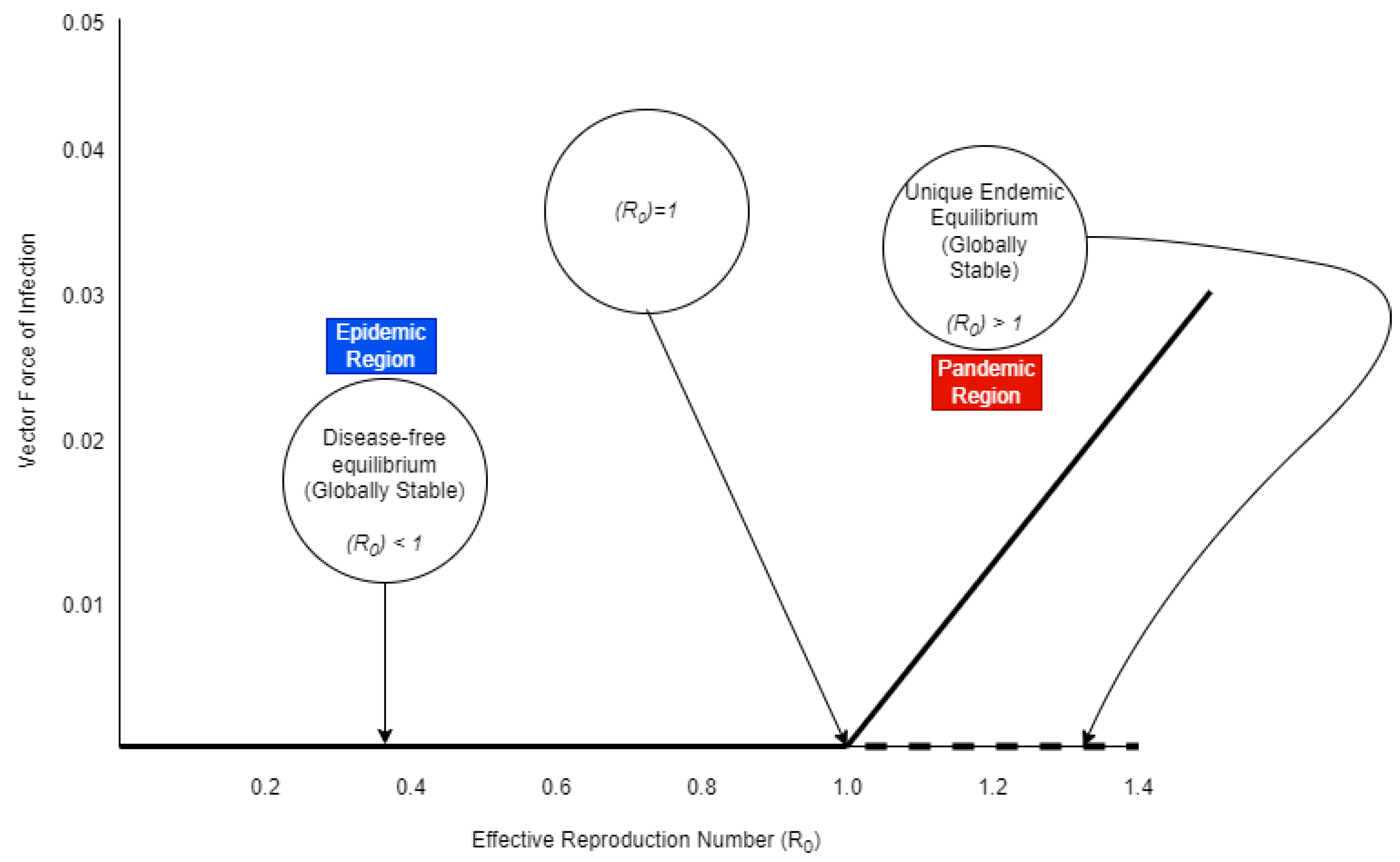
Figure 1. Forward Bifurcation plot of the Onchocerciasis model.
Mathematics 12 00222 g001
Figure 2. Simulation of the population state with varying parameters of onchocerciasis model dynamics, (left): α h = 0.09 , γ h = 0.01 , r = 0.05 , (right): α h = 0.05 , γ h = 0.09 , r = 0.0667 .
Mathematics 12 00222 g002
Figure 3. Susceptible and exposed human population. (a) Dynamic behavior of susceptible human population with varying parameters and (b) Dynamic behavior of exposed human population with varying parameters.
Mathematics 12 00222 g003
Figure 4. Infected and recovered human population. (a) Dynamic behavior of infected human population with varying parameters and (b) Dynamic behavior of recovered human population with varying parameters.
Mathematics 12 00222 g004
Figure 5. Graph of parameters and their sensitivity indices.
Mathematics 12 00222 g005
Figure 6. Graph of parameters and their sensitivity indices.
Mathematics 12 00222 g006
Table 1. The description of parameters of the onchocerciasis model.
SymbolsDefinitions
Ψ h ( x i ) Term of recruitment for susceptible individuals at a discrete age x i
Ψ v Term of recruitment for the susceptible vectors
δ Vector’s rate of biting
λ h ( x i ) Probability that a human will contract a disease at a specific age x i as a result of being bitten by an infectious vector
λ v Probability that a bite will cause a parasite to spread to a susceptible vector
μ h ( x i ) Human mortality rate per capita at a discrete age x i
μ v Per capita vector death rate
γ h ( x i ) Human disease-related mortality rate at a given age x i .
γ v Rate of disease-induced vector mortality
α h ( x i ) Per capita rate at discrete age x i of human progression from the exposed state to the infectious state
α v The rate at which vectors move from an exposed state to an infectious state per person
r ( x i ) Percentage of individuals who, after treatment, go from an infectious state to a recovered state at a discrete age x i
ω ( x i ) At each discrete age x i , the per capita transition rate from the recovered human condition to the susceptible state
ν h ( x i ) Factors that prevent sickness in humans at specific ages x i .
ν v Factors that suppress illness in vectors
Table 2. Parameter values.
SymbolsValueSource
Ψ h ( x i ) 0.459Estimated
Ψ v 0.4Estimated
λ v 0.758[10]
λ h ( x i ) 0.8354[11]
α h ( x i ) 0.5[12]
α v 0.6[13]
γ h ( x i ) 0.09[10]
γ v 0.085[10]
δ 0.08[10]
μ v 17.3809[11]
μ h ( x i ) 0.01567[11]
ω ( x i ) 0.05[12]
ν h ( x i ) 0.01[12]
ν v 0.013[13]
r ( x i ) 0.0667[13]
Table 3. Parameter Sensitivity Index for R h .
ParametersSensitivity Index
δ 1
λ h ( x i ) 1
Ψ h ( x i ) 1
μ h ( x i ) 1.05749081780538
α h ( x i ) 0.0395138311016970
r ( x i ) 0.100955636880930
γ h ( x i ) 0.881067376415387
Table 4. Parameter Sensitivity Index of R v .
ParametersSensitivity Index
δ 1
α v 0.978554014717723
λ v 1
Ψ v 1
μ v 2.93623530191190
γ v 0.0423187128058188
Disclaimer/Publisher’s Note: The statements, opinions and data contained in all publications are solely those of the individual author(s) and contributor(s) and not of MDPI and/or the editor(s). MDPI and/or the editor(s) disclaim responsibility for any injury to people or property resulting from any ideas, methods, instructions or products referred to in the content.