Article

Visualizing Convergence Dynamics across Regions and States: h-Convergence

1
King’s Business School, King’s College London, 30 Aldwich, London WC2B 4BG, UK
2
SEAM, University of Messina, Piazza Pugliatti 1, 98100 Messina, Italy
Mathematics 2024, 12(2), 256; https://doi.org/10.3390/math12020256
Submission received: 18 December 2023 / Revised: 8 January 2024 / Accepted: 9 January 2024 / Published: 12 January 2024
(This article belongs to the Special Issue Mathematical and Statistical Modeling of Socio-Economic Behavior)

Abstract

:
Researchers interested in studying whether convergence dynamics are in place among regions within the same country have adopted both statistical tools and empirical frameworks developed when studying convergence across different economies. We show that this approach is risky, because when an analysis is conducted at the regional level, the absolute and club convergence processes are more likely to co-exist than in the case of world economies. We propose an empirical approach where the two hypotheses are not taken as competing. Our procedure uncovers periods of convergence and periods of divergence for the three samples we studied: Italy observed at both the regional and provincial levels; EU regions; and world economies. We find a process of absolute convergence for Italian regions from 1951 to 1999, and that their convergence process ends in 1971 after a period which we define as clustering convergence. We also find a process of convergence across European regions from 1977 to 1993; that ends in 1985 in favor of a process of clustering and divergence. Finally, our procedure uncovers a process of absolute convergence from 1964 to 1975 and divergence from 1975 to 1999 in the case of world economies.

1. Introduction

Researchers studying whether club convergence dynamics and/or absolute convergence processes occur among regions within the same country adopt both statistical tools and empirical frameworks developed when studying convergence across different economies—among many others, see Gonzalez-Paramo and Martinez-Lopez (2003) [1], Lima (2010) [2], Kholodilin, Oshchepkov and Siliverstovs (2012) [3], Goech and Huter (2016) [4], Puente (2017) [5], Eichengreen (2019) [6], Lehmann, Oshchepkov and Silvagni (2020) [7], Savoia (2020) [8] and Ram (2021) [9].
The approaches above take the Absolute Convergence Hypothesis (ACH hereafter) and the Club Convergence Hypotheses (CCH hereafter) as nested hypotheses, in the sense that evidence in favor of the former is taken as evidence against the latter and vice versa. To the best of our knowledge, none of the authors studying regional convergence asks whether, or subsequently how, the empirical framework should be adjusted in the case of analysis of convergence processes at the regional level—that is, when a different level of aggregation is of interest. When examined closely, this testing strategy is potentially risky. Indeed, observations at the regional level are much more likely to be dependent upon each other than in the case of world economies. Regions within the same economy share not only commercial flows, political relationships, and migration dynamics as world economies do, they also share culture, institutions, natural resources, luck, and government policies; in short, they share all the characteristics that are defined as new engines of growth according to the new growth theory (Acemoglu 2009 [10]).
The above raises several considerations when the analysis of regional convergence processes is of interest. At the regional level, observations that are geographically close or at a similar level of development are likely to converge with each other—that is, likely to generate one cluster of observations—before eventually converging with regions that are geographically distant or at different stages of development. In turn, this means that studies examining regional convergence are more likely to conclude in favor of club convergence and against absolute convergence compared to those studying samples of world economies. Indeed, because the speed of convergence among similar or closer regions is likely to be faster than that among all regions, key absolute convergence dynamics may be overshadowed.
To illustrate our argument above with a real example, we applied the framework proposed by Quah (1997) [11] to the case of Italian regions. For this sample of regions, we showed that the existing clustering dynamic does not necessarily exclude the more general underlying absolute convergence process, and vice versa. Furthermore, we also found that if the two hypotheses are taken as competing processes, the analysis is likely to lose some essential information on when the clustering and/or convergence processes began and/or ended. Therefore, this has clear implications when investigating the reason why these processes ended or began.
Our results support the development of an approach where convergence processes are not assumed to be similar among samples of economies at different levels of aggregation; in addition, they call for a testing procedure that allows us to study the ACH and the CCH independently of each other. To this aim, in the current study we build on non-parametric density estimation and critical smoothing techniques. We show that convergence processes can be studied by means of the critical bandwidth for unimodality, rather than the critical amount of smoothing for bimodality as initially proposed by Bianchi (1997) [12]. The procedure we propose identifies periods where economies experience club and absolute convergence, as well as periods where economies experience club convergence and divergence.
We apply our procedure to four samples of economies, including Italian regions, Italian provinces, EU regions, and a sample of world economies. Our aim is not to study whether these economies convergence, cluster, or diverge over time, as excellent research on these questions already exists. Instead, we aim to propose an empirical approach that can help visualize convergence dynamics, clustering, and divergence processes over time, so as to provide policymakers with information on when observations will eventually converge, cluster, or diverge—information that should be considered key as far as policy decisions are concerned.
Our results show that the distribution of per capita GDP for these samples of observations does not randomly fluctuate. We find that there are periods of convergence and clustering as well as periods of divergence and clustering. More specifically, we find a process of absolute convergence and club convergence for Italian regions between 1951 and 1999. In contrast with the relevant literature, we also find that the convergence process in Italy ends in 1971, after a period of what we define as clustering convergence—that is, observations cluster in groups that converge until 1971, when government public intervention ends. We also find a process of convergence across European regions between 1977 and 1993. In this case, the convergence process ends in 1985 in favor of a process of clustering and divergence. Interestingly, the procedure we propose also uncovers a process of absolute convergence between 1964 and 1975, followed by divergence between 1975 and 1999, in the case of world economies, despite all the distributions displaying a bimodal shape. The testing procedure we propose is robust to log-transformations, which are relevant across convergence and growth studies, where variables are typically log-linearized before analysis is performed.
The remainder of the paper proceeds as follows. In Section 2 we present the data and motivate our analysis by showing that the results of convergence dynamics analysis may be misleading when analysis approaches proposed for economies are applied to regions. The discussion will also show that the CCH and ACH are not necessarily competing hypotheses. This conclusion suggests developing an empirical methodology where the two hypotheses are de-nested. Section 3 presents our testing procedure. Section 4 reports the empirical results, and Section 5 provides some concluding remarks.

2. Convergence Dynamics for Regions and States: Challenges

2.1. Data

We build our discussion on the time evolution of the relative GDP per capita for three economies, although the analysis of convergence dynamics could build on other metrics, such as human capital or institutional convergence. However, the main discussion in the field revolves around GDP, so we prefer to use this variable. Our three samples include (i) Italy, observed at the regional level over the sample period 1951–1999, and observed at the province level over the sample period 1970–1999; (ii) EU regions over the sample period 1977–1993 and (iii) a sample of world economies observed from 1960 to 2000.
Among many others, the sample of Italian regions has been recently adopted for the study of convergence dynamics and processes by Fanti, Pareira, and Vigillito (2023) [13]—see also the references of this paper. In our view, this database is especially interesting in three respects. First, it represents the only sample—at least among those studied in this paper—where the distribution of incomes per capita moves in the direction suggested by Quah (1997) [11] and Bianchi (1997) [12], among others: the distribution of relative income per capita goes from unimodality to bimodality. However, especially during the mid-1950s to the mid-1970s, that Italian regions converge with each other is evidence that is not in question. Secondly, the cross-sectional dimension of the sample is small—twenty regions. In turn, this dimension is similar to the dimension of the sample used by Silverman (1981) [14] when designing a test for multimodality that builds on the idea of critical smoothing. Hence, we show that the empirical approach we propose allows for the analysis of small samples. Finally, to our knowledge, when this database has been used to perform distribution-based analyses of convergence papers generally conclude against absolute convergence (Terrasi 1999) [15].
The sample of Italian provinces is of interest in the context of the current study as a means of checking whether results confirm, or disconfirm, the analysis that builds upon regions by drawing on a larger and more volatile sample. Specifically, Italy had 95 provinces during the period under analysis. Rich regions contained some poor provinces, and some rich provinces were located in poor regions. This sample contains smaller observations within regions. The number of provinces increased over time to 103; these new provinces came from the disaggregation of existing provinces. For these reasons, the sample of provinces is more likely to exhibit lower persistency than the regional sample (for a more recent set of data on these questions, see Calcagnini and Perugini 2019 [16]).
The sample of EU regions is of interest in the context of the current study because some studies concluded in favor of convergence across the EU at the national level (Quah, 1993 [17]; Barro and Sala-i-Martin, 1991 [18]); however, at the regional level, disparities among per capita incomes seem to persist (Goech and Huter 2016 [4]). It is therefore of interest to study whether these contrasting results depend upon the different levels of aggregation of the observations, on larger cross-sectional dimensions, or because different sample periods are analyzed in different papers.
Finally, we adopted the sample of world economies to study absolute convergence and divergence processes using the sample adopted by Quah (1997) [11]. This sample of economies has been analyzed in many respects using many different econometric tools. What the results of existing studies indicate is that world countries are converging to different steady state levels, and that the distribution of per capita GDPs fluctuates over time (see, among the many others, Canova and Marcet, 1995 [19]; Bernard and Durlauf, 1995 [20]; Quah, 1996 [21]). Although the debate about cross-country convergence has slowed down considerably, Kremer et al. (2021) [22] and Patel et al. (2021) [23] recently proposed some challenges in favor of the ACH; in turn, this evidence has contributed to refueling the convergence debate somewhat.

2.2. Can Absolute and Club Convergence Co-Exist? The Case of Italian Regions

Quah (1997) [11] suggests studying convergence dynamics by analyzing the evolution of the shape of the distribution of income per capita estimated for different years across a cross section of economies. If the evidence suggests that the distribution evolves from a bimodal distribution to a unimodal distribution, then we can conclude that economies are converging to each other. This is because the number of modes informs about the presence of a given number of clusters in the distribution, which in this case would be collapsing to a single group. In contrast, if the shape of the distribution evolves from a unimodal to a bimodal distribution, then we observe “twin peaks” dynamics. In this case, we would observe convergence within the different clusters of economies, but divergence between clusters because the middle class tends to vanish. In other words, the study of the evolution of the shape of the distribution of the income per capita across countries allows for the study of convergence processes. In this approach, the ACH and the CCH are taken as nested hypotheses, because evidence in favor of the ACH is taken as evidence against the CCH and vice versa.
Because we are interested in estimating the shape of the distributions of income per capita, we follow Rosenblatt (1956) [24], which defines the following class of non-parametric estimators:
f ^ n , h = 1 n h i = 1 N K x x i h ,
where N are the cross-sectional realizations of income per capita; h is the positive window width, or bandwidth; and K(·) is the kernel function that provides the estimate of the density function of the random variables x, estimated at the point x = x0 as the weighted sum of all the observations. The weight for the ith income per capita, xi, is given by the function K(·). The approach defined in Equation (1) is called a non-parametric approach, essentially because it is seen as opposed to estimating various moments (parameters) of the distribution and substituting them into an a priori distribution. Instead, this approach entails estimating a continuous histogram, so that the data speaks for themselves.
An obvious criticism of the approach above is that distributions are estimated independently of each other. Therefore, it does not inform about who is going where in the distribution of incomes over time. This is a major drawback, as ideally, we would like to know how much the current positions in the distribution of incomes depend upon the initial positions—that is, what are the chances that poor economies “take off” and converge with richer economies, and subsequently, how long will it take for this to happen? To this aim, Quah (1997) [11] proposed that once the analysis above is complete, the so-called stochastic kernel, which informs about persistence and mobility dynamics in the distribution of incomes, should be estimated. The stochastic kernel provides an estimate of the probability that observations change or stay in the same position at t + s, conditional to their initial position at t:
f ^ y t + s y t = f ^ y t + s , y t f ^ y t .
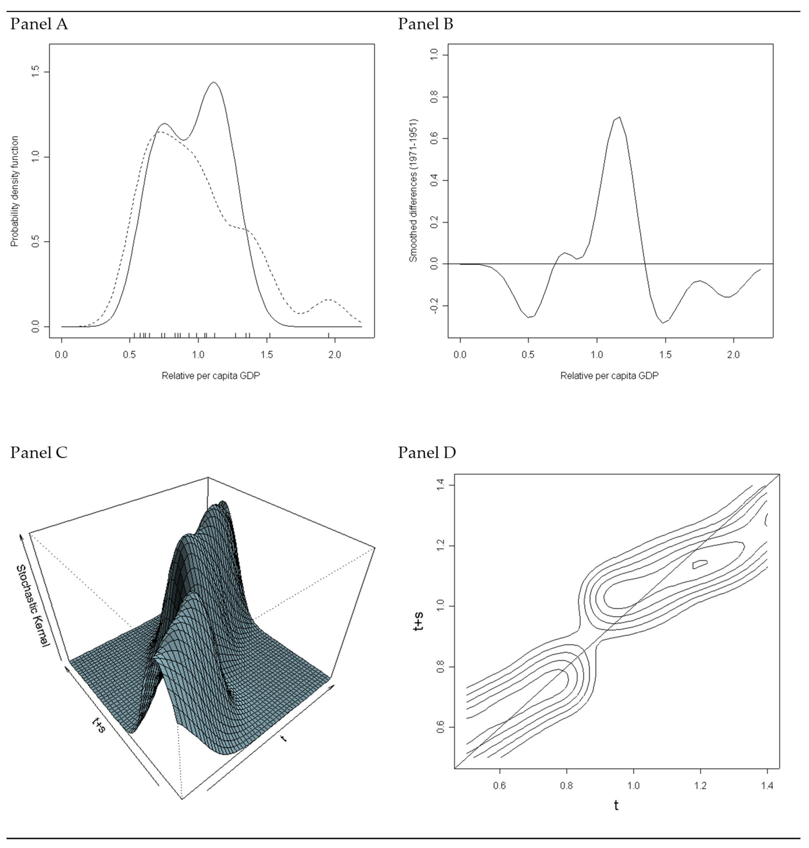
This analysis of Equation (2) informs whether rich economies at t are still rich at t + s (in this case one would observe persistence); if some poor economies at t are rich at t + s (in this case one would conclude in favor of mobility) or if some groups of the economies that are close together at t separated because of a process of divergence (in this case one would conclude in favor of separability). Vectors t and t + s are obtained as in the standard transitional matrix approach. We expect that the lower the s, the higher the persistence, given the somewhat high memory that income per capita typically have (Caggiano and Leonida, 2009) [25]. We have performed the analysis as suggested by Quah (1997) [11] for the case of Italian regions. Results are reported in Figure 1.
In Panel A, we report the estimate of the distribution of incomes per capita across Italian regions for 1999 and 1951; to ensure comparability, the estimates were obtained by using the same kernel and the same bandwidth, averaged over all the years, and calculated under the hypothesis that the data were normally distributed—our conclusions did not qualitatively change as these parameters changed.
Our results supported the conclusion that the regional economies did cluster in groups. The shape of the distribution of incomes evolved from unimodality to bimodality; in turn, this evidence must be taken as being in favor of the existence of two basins of attraction in the distribution of incomes in the Italian region. This evidence was taken as being against the absolute convergence process and in favor of club convergence dynamics. In other words, we concluded that regional Italian economies did not converge to each other, but that they converged in groups.
The analysis of the stochastic kernel confirmed this conclusion and informed about who was converging with who. As an illustrative example, we set s = 15; that is, we studied transition within 15 years—again, conclusions were robust to this decision. The results reported in Panel B suggest that two modes are emerging in the distribution of incomes. By looking at the contour plots reported in Panel C, we can appreciate that these basins of attraction are close to the 45-degree line. However, not all the basins of attraction are stable long-run equilibria. To see this, we superimposed a theorical accumulation function, which showed that the accumulation function crosses the 45-degree line from above for the first and the last crossing, and from below for the basin of attraction located in the middle of the 45-degree line. This suggests that the latter is an unstable equilibrium. The arrows in the phase diagram help to understand the point discussed here—see Caggiano and Leonida (2013) [26] for a discussion of the dynamic). For this reason, the middle class is vanishing, which is exactly the evidence that is needed to conclude, according to Quah (1997) [11], against the absolute convergence hypothesis, and in favor of the club convergence hypothesis.
When examined in more detail, the results reported in Figure 1 suggested something more: that the variance of the observations reduced quite substantially. In other words, in 1999 observations were closer that they were in 1951. This can be partially explained: soon after World War II, Italian regions experienced a convergence process, mainly attributable to the central government making an effort to finance public projects aimed at helping the southern and central regions catch up with those located in the north of the country—the so-called “extraordinary intervention.” However, whether the convergence process in fact happened, when it eventually concluded, and when the two basins of attractions emerge are of obvious interest to both the researcher and the policymaker. However, these are all hidden if the analysis of the stochastic kernel is adopted tout court.
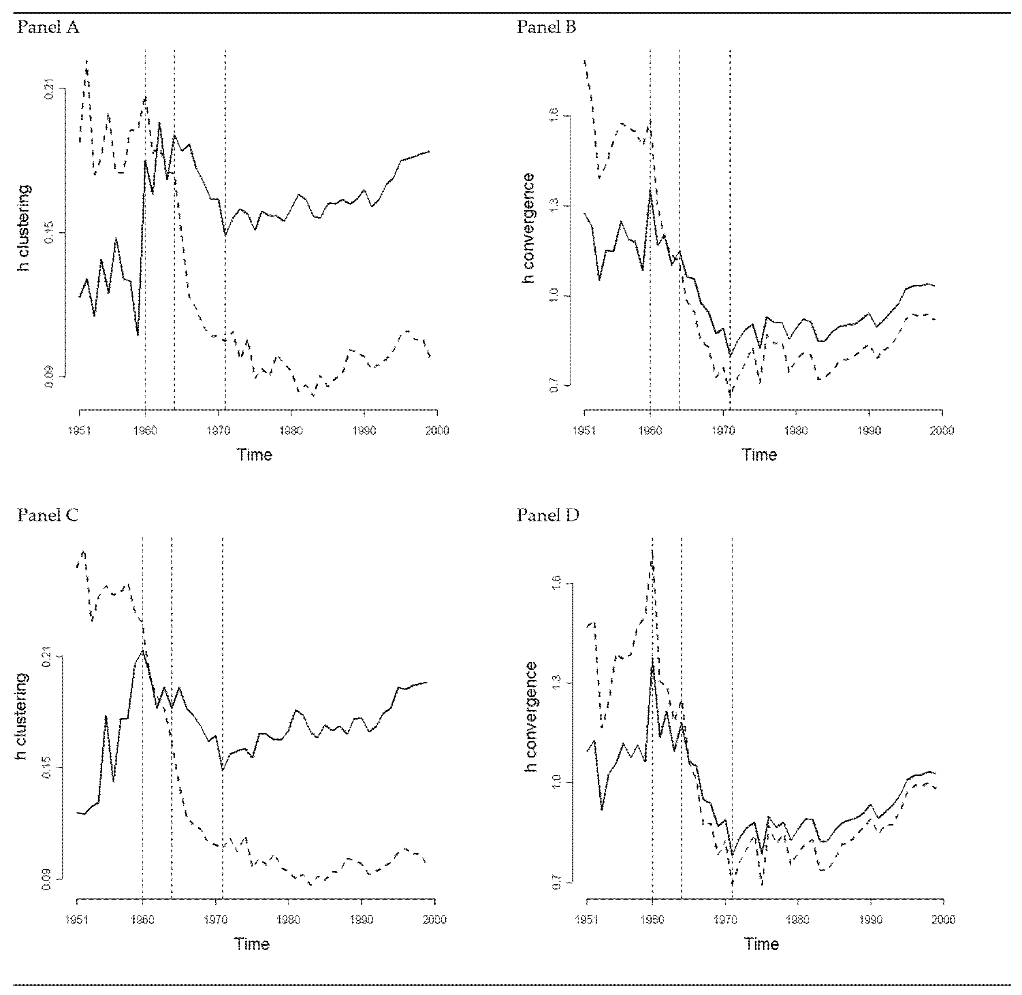
Furthermore, the absolute convergence process that we discussed above would be somewhat obscured if we adopted the analysis proposed by Quah (1997) [11] for the 1951–1971 period only; the reason why we are cutting off the sample period at 1971 will be clearer later. Results of the analysis are reported in Figure 2. For comparability, we kept all the details of the estimation constant, including the kernel and the bandwidth. In Panel A, the bimodality of the distribution emerges and, despite being much less pronounced when compared to the results reported for the period between 1951 and 1999, it supports the club convergence hypothesis. At the same time, the variance of the distribution reduces drastically, in favor of the absolute convergence hypothesis. The co-existence of the two processes—both absolute and club convergence dynamics—is evident by taking the smoothed difference between the distribution in 1971 and that in 1951, as reported in Panel B. The smoothed difference clearly shows that observations moved from the tails of the distribution to its center; some of them converged with rich regions and others with poor regions.

3. Research Design

A similar conclusion can be reached by looking at Panel C and Panel D, where we report the analysis that builds on stochastic kernels—as estimated above by building on a 15-year transition. Here, the two basins of attraction are evident and are close to the 45-degree line. Also, the middle class is vanishing over time. The evidence would therefore disconfirm the ACH in favor of the CCH, despite all the relevant literature that concluded in favor of the ACH for Italy over this period. This is further confirmed by examining the range of the observations, which at t is much higher than the range at t + s. Therefore, this evidence is clearly in favor of the absolute convergence hypothesis.

3.1. De-Nesting ACH and CCH

Our results show that evidence in favor of a bimodal distribution of incomes would not necessarily contradict an absolute convergence dynamic, and that two groups of economies existing within the income distribution does not provide sufficient evidence to reject the ACH, per se. Specifically, the bimodality of the distribution informs about the number of groups present in the distribution of incomes; however, groups may converge over time. It is reasonable to expect that similar economies, or economies that are geographically closer, converge more rapidly with each other than with those that are either at different levels of development or geographically more distant. In the latter case, we may observe both clustering processes and convergence dynamics.
It is noteworthy that the approach under which the presence of clubs in the distribution of incomes is necessarily evidence against the ACH also does not find theoretical support. Caggiano and Leonida, (2013) [26] and Leonida (2023) [27] discuss theoretical reasons why a club convergence pattern may be consistent with both absolute divergence and convergence dynamics. This is even more pertinent for regions, where observations are much more likely to be dependent upon each other than in the case of the world economies—actually, because of commercial flows, political relationships, and migration dynamics, among others, the hypothesis that world economies are independent should be examined carefully as well. Regions share culture, institutions, natural resources, luck, and government policies: in essence, all the characteristics defined as the new engine of growth according to Acemoglu (2009) [10].

3.2. A Bandwidth-Based Test for Convergence

The evidence that we have discussed above and the conclusions we have reached call for an empirical analysis where absolute and club convergence processes are not taken as competing hypotheses. To this aim, we build on Bianchi (1997) [12] that suggested interpreting the test for multimodality proposed by Silverman (1981) [14] as a test for convergence. Silverman (1981) pointed out that the magnitude of h, in Equation (1), determines which observation we are looking at. If the value of h is small, the kernel gives a meaningful weight only to the observations close to x₀, with the result that the density function is insufficiently smoothed. If h is s too large, the kernel also assigns a weight to observations too far from x0, leading to over-smoothing of the distribution and a loss of crucial information about the true underlying shape of the distribution. Therefore, bandwidth magnitude is the crucial parameter for the effective estimation of density.
Bianchi (1997) [12] suggested interpreting the magnitude of the so-called critical bandwidth for unimodality as a test of convergence. The critical bandwidth, h c , is defined as the smallest smoothing parameter for which the estimated density displays m modes, and therefore informs about the presence of m clusters in the distribution of incomes. To reduce the arbitrariness associated with the choice of the smoothing parameter, Bianchi (1997) [12] suggested that we should apply the critical bandwidth amount of smoothing defined as:
h c = i n f h : f ^ n , h   h a s   a t   m o s t   m   m o d e s ,
According to the author, “this idea of critical smoothing is naturally related to hypothesis testing and to multimodality test. Indeed, if the true underlying density has two modes, a large value of h c is expected, because a considerable amount of smoothing is required to obtain a unimodal density estimate from a bimodal density” (Bianchi 1997:203). Therefore, provided that the Gaussian kernel is used, and that estimates have monotonicity of features (peaks and valleys) with respect to the amount of smoothing, the number of modes is a decreasing function of the bandwidth magnitude. The Gaussian kernel is indeed a weighting function for which the number of zero crossings of the smoothed derivative is always a decreasing function of h—see Silverman, 1981 for a formal proof of this property. Because of this property, we have used this kernel in the previous sections and in the subsequent analysis.
Bianchi (1997) [14] proposed recovering some point-in-time densities, estimated by applying the critical bandwidth for bimodality, and then testing the significance of their shape against the null hypothesis of unimodality by means of bootstrap techniques. The achieved significance levels are then compared over time; if the strength of rejection of the null hypothesis increases over time, this would be evidence against the ACH.
There are four main issues in interpreting the test as Bianchi (1997) [14] suggested. First, where the null of absolute convergence is rejected, no information is given. We are unable to assess whether observations are diverging, whether they are clustering, or both. No information is provided, moreover, about the dynamics occurring between the years chosen to bootstrap the samples, or in which particular year the convergence process stops or begins. Third, the procedure is not robust to log-transformations; when per capita incomes are log-transformed, the unimodal shape of the density is never rejected at standard levels of significance. This problem is particularly important in the β-convergence literature, where this transformation is usually done before testing for convergence. Finally, Bianchi (1997) [14] suggests comparing p-values obtained from different amounts of smoothing. However, comparisons between distributions should be performed only when the same amount of smoothing is applied to the estimates (Marron and Schmitz, 1992) [28]. It is not easy to compare distributions over time; consequently, comparisons between p-values obtained as suggested are risky.

3.3. The De-Nested ACH and CCH in the Non-Parametric Setup

Because of these shortcomings, we suggest using the critical bandwidth in a different manner. Our starting point is recognizing that both the ACH and CCH have natural counterparts in the non-parametric framework. From the σ-convergence framework we know that, under the hypothesis that the steady state distribution of incomes exists, for a set of countries to converge the variance should approach a constant positive value. We know that the variance does not provide enough information for testing for club convergence processes; however, it does inform about absolute convergence dynamics. Moreover, the underlying reasoning may be applied to the critical smoothing parameter.
More specifically, the critical amount of smoothing for unimodality may be employed as a measure of clustering, and so it may provide a test for the CCH. If the steady state distribution exists, it has its equilibrium critical bandwidth for unimodality, h c , towards which the measured critical bandwidth for unimodality, h c t , tends. The critical bandwidth, used in conjunction with the Gaussian kernel, is of interest in this context because it depends upon the number of clusters that the distribution displays, their position in the distribution, and on the dispersion that each cluster displays. Because of the monotonic relation between the bandwidth magnitude and the number of modes—provided by the use of the Gaussian kernel—if the minimal amount of smoothing increases, clusters become increasingly pronounced over time, providing evidence in favor of the CCH. Conversely, a reduction in the critical amount of smoothing signals that clusters are collapsing; in such a case, evidence against the CCH would be found.
Moreover, if this series displays an upward break, a much higher amount of smoothing is necessary to obtain a unimodal distribution from a sample that is composed of two clusters. Such a break informs us about the two groups co-existing in the sample in the year the break manifests—in favor of the CCH. Conversely, a downward break informs about two groups collapsing—evidence against the CCH.
The analysis of the h c t series informs on clustering. However, just as the variance does not provide information on clustering, this index does not provide information on the dispersion of the entire sample of observations. As a test for the ACH, we suggest averaging both the h c t series and the sample variance, σ t . This average metric informs whether the clustering dynamics as measured by the h c t series is offset by changes of the variance in the opposite direction, or if changes in the variance go along with a club convergence process. More importantly for our aims, the comparison between these two indices provides information on whether and when the absolute and club convergence processes begin or end in the period of analysis.

3.4. h-Convergence

Let y i t } be the realizations of relative per capita GDP for i = 1, …, N economies, where t = 1, …, T is the time span of interest. Assume that the following questions are of interest:
How many long-run equilibria does the sample of economies have?
Do observations in the same group catch up with each other, and at which eventual point in time?
Do observations converge to one another, and at which eventual point in time?
To answer the questions above, we suggest the following three-stage procedure:
1.
Estimate the critical bandwidth for unimodality and the optimal bandwidths—for example, the Least Squares-Cross Validation bandwidth (Silverman, 1986 [29]) or the smoothing parameter proposed by Scheather and Jones (1991) [30].
2.
Extract the following metrics from each distribution of incomes per capita:
i.
A metric of the optimal bandwidth, h o t , under one chosen criterion, o b t :
o b t = ( h o t T / 1 T h o t ) .
ii.
A metric of the critical bandwidth, h c t , taken as a metric of clustering, c t :
c t = ( h c t T / 1 T h c t ) .
iii.
A metric of the sample variance, ν t :
ν t = ( σ t T / 1 T σ t ) .
iv.
The average of the metrics defined in ii and iii, l t :
l t = 1 2 ( c t + ν t ) .
3.
Analyze the series o b t ,   c t ,   ν t , and l t and their time evolution. The comparison between the index o b t , and c t informs about whether the critical amount of smoothing lies above or below the optimal bandwidth, and it also therefore provides information about the shape of the distribution. This defines the number of groups and modes that the sample displays.
3.1.
Statement 1: if o b t , c t then the distribution has two clusters of observations.
3.2.
Statement 2: if c t 1   c t then the clusters are diverging. The series c t informs about club convergence dynamics—h-clustering. In the case of a positive trend, we can conclude in favor of divergence between groups; that is, in favor of the CCH hypothesis.
3.3.
Statement 3: if l t 1   l t then the economies are diverging. The series l t informs about whether clustering is offset by reduction in the variance and therefore informs about whether the absolute convergence process is in place—h-convergence.

4. Empirical Results

4.1. Convergence and Divergence across Italian Regions

Figure 3 reports the results for the analysis of convergence across Italian regions. In Panel A, the solid line plots the behavior of the c t metric over time, and the dashed line plots the behavior of the o b t metric—where the optimal bandwidth is defined by the Scheather and Jones (1991) [30] parameter. In presenting our results we adopt the Scheather and Jones (1991) [30] smoothing parameter as the optimal reference bandwidth—results do not qualitatively differ by using the smoothing parameter given by the Least-Squares Cross Validation method. In Panel B the solid line plots the behavior over time of the h-convergence metric, and the dashed line plots the variance over time.
The results suggest that the value of the h-clustering index in 1951 is lower than the optimal smoothing parameter, while the opposite holds for the distribution in 1999. The evidence suggests that the distribution is unimodal in 1951 and bimodal in 1999. Moreover, the value of the clustering index in 1951 is lower than the value in 1999. Taken together, the evidence suggests that regional economies clustered across years, which is in favor of the CCH.
The results in panel B show that the opposite is true for the h-convergence measure. The index is higher in 1951 than in 1999. The evidence suggests that regions are closer in 1999 than they are in 1951. Therefore, if taken as a whole, the analysis suggests that this period should be considered a period where regions experienced absolute convergence. This conclusion holds despite evidence that regions experienced marked clustering over time. Results are in favor of both the CCH and the ACH. The two h metrics confirm the intuition behind the estimates reported in Figure 1 and Figure 2—namely, that the distribution estimated for 1999 shows two distinct modes and groups, and that the distribution in 1951 displays a higher variance.
However, the entire period may be divided into four sub-periods—namely 1951–1960, 1961–1964, 1965–1971, and 1972–1999. In the first of these periods, regions tend to cluster and diverge. The strength at which regions polarize dominates the observed reduction in the variance. In 1960 the h-clustering metric shows an upward break and, because in this year the metric lies in the region of the space where unimodality is rejected, this suggests that the distribution shows two groups of regional economies from 1960 onwards. However, the two modes are still close to each other; indeed, the critical bandwidth for unimodality is still close to the optimal reference bandwidth. From 1960 to 1964 the two groups are more and more defined. The h-clustering index increases and is higher than the optimal smoothing parameter. Moreover, the h-convergence index decreases. In this period, therefore, regions both converge and cluster; the two modes become increasingly significant. From 1964 to 1971 the two groups converge: both the h-clustering and the h-convergence metrics decrease. The results lead to a different conclusion if we look at the period from 1971 to 1999, however. Over this sample period, regions both cluster and diverge, and so support the hypothesis that the two processes are mutually exclusive.
This analysis of the Italian region offers some conclusions that contrast with those proposed in the literature about convergence in world economies. Indeed, if taken as a whole, our results support the hypothesis that the two processes—namely, the absolute convergence and the club convergence dynamics—may or may not occur together. For this reason, the two processes, at least in the case of regions, should be taken as competing processes. Our results also differ from previous findings in the literature on regional Italian convergence processes. More specifically, our results suggest that the convergence process ended in 1971, rather than in 1975 or 1973 (Mauro and Podrecca 1994 [31], Paci and Saba 1998 [32]; Terrasi 1999 [15]). From 1971 to 1999, regions both diverge and cluster, with a mass shift in 1991.
Results from the procedure we are proposing are robust to the log-transformation of income per capita. This transformation is particularly important for convergence and growth studies, as data are usually log-transformed when estimating the β-convergence parameter—this is due to the log-linearization approach around the steady state equilibrium. We consider the following transformation of the data:
z i t = l n   ( y i t )
where y i t is the income per capita in the i-th economy. Once transformed to logarithms, we estimate our metrics again by using the transformed data and duplicate the entire analysis. Results are reported in Panels C and Panel D of Figure 3. The results do not substantially change, contrary to the testing procedure proposed, for example, by Bianchi (1997) [12] and Terrasi (1999) [15].

4.2. Divergence across Italian Provinces

Figure 4 reports the analysis for the sample of Italian provinces. From the administrative perspective, provinces belong to regions and are smaller in terms of population size. Because we obtained smaller and more volatile observations from the regions, the twin peak shape of the Italian distribution is almost insignificant in 1970: the value of the critical bandwidth for unimodality is lower than the value of the smoothing parameter that we are using as a reference. This is because some rich provinces are located in poor regions, and some poor provinces are located in rich regions. As a result, the well-known dualistic nature of the Italian economy is hidden, especially if the approach building upon estimates of the distribution of incomes is adopted acritically.
The results suggest that the values of both the h metrics are higher in 1999 than in 1971. Therefore, over the period from 1971 to 1999 we observe an increase in the divergence and clustering process. However, the dynamics we observe over the entire period may be split into three sub-periods. The first period ends in 1971, consistent with evidence from the regional sample analysis, where we found the end of the process which we named clustering convergence. In the second period, which spans from 1971 to 1990, the sample of provincial observations both cluster and diverge. In 1991 both metrics, as well as the variance, display a break—this mass shift was present, with less strength, in the regional case as well.
This break is informative about a mass shift from one cluster to another—a simple inspection of the data shows that a small number of provinces move from the rich to the poor cluster—not reported here for the sake of brevity. However, this shift is not enough for the twin peaks to disappear. The critical smoothing parameter is located in the region of the space where the distribution is bimodal. The divergence and clustering dynamics resume, once again, until 1999.
The dynamics relating to this sample of economies also helps explain why the literature focusing on the Italian divergence process dates the end of the absolute convergence process at 1975. Indeed, the variance of both the regional and especially the provincial samples show a valley in 1975; however, from the viewpoint of the metrics we have proposed, in 1975 regions and provinces experienced a somewhat short-run fluctuation within the more general process of divergence and clustering. This fluctuation is similar to some of the fluctuations that follow—for example, those in 1977 and 1985. Our results confirm that the reversal in the convergence paths of Italian regions and provinces took place in 1971 instead.

4.3. Are European Regions Converging?

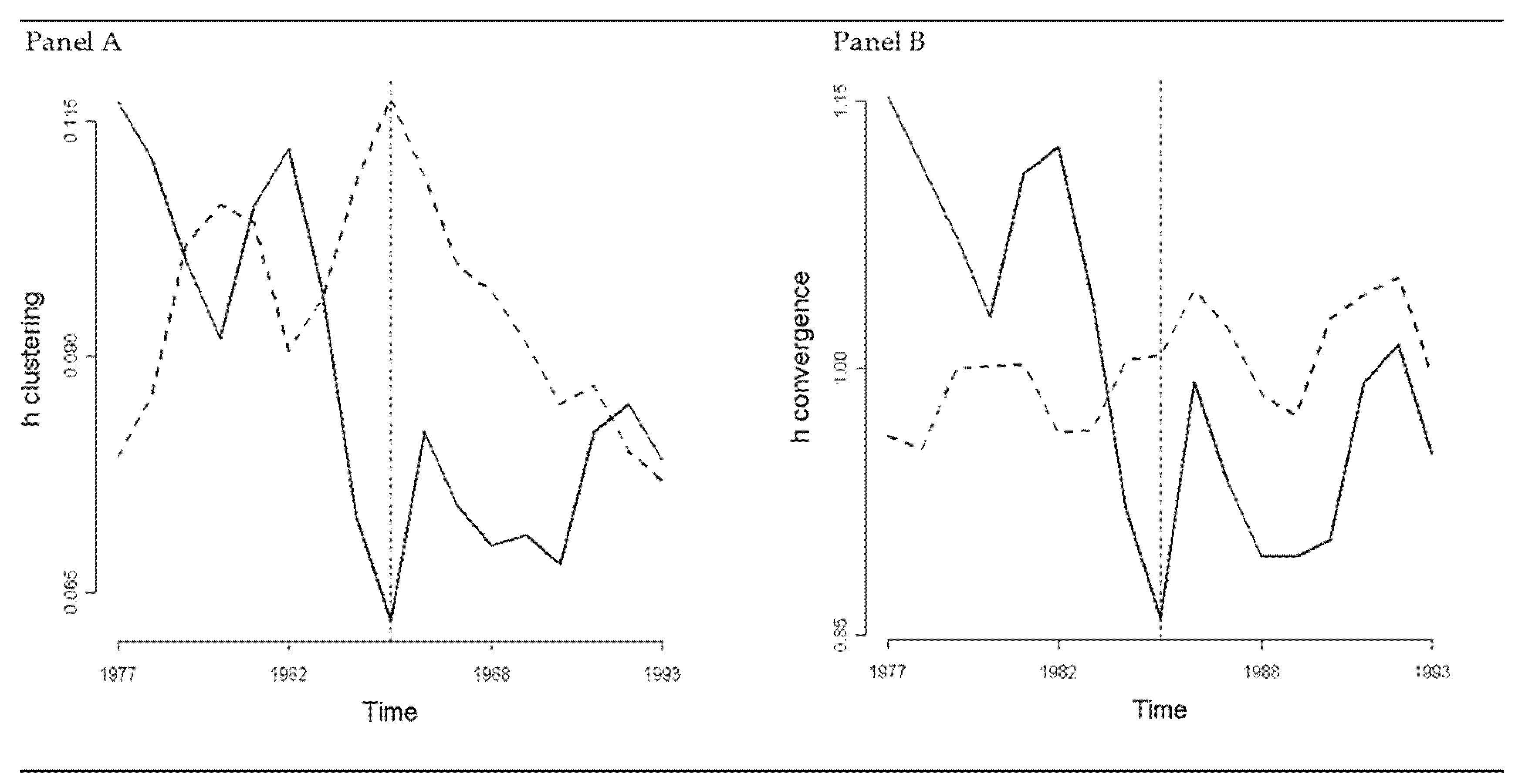
Estimates of the four metrics relative to EU regions are reported in Figure 5. As above, the solid line in Panel A reports the h-clustering index and the dashed line reports the series of the optimal bandwidth as defined as Scheather and Jones (1991) [30], while the solid line in Panel B reports the h-convergence index and the dashed line depicts the plot of the variance.
The results in Panel A suggest that the optimal smoothing parameter in both 1977 and 1993 is lower than the reference optimal bandwidth. The evidence is in favor of bimodality for this distribution of incomes per capita in the EU. However, for most years the unimodality of the distribution of incomes cannot be rejected. Moreover, the h-clustering metric is higher in 1977 than in 1993; in turn, this evidence suggests that clustering tends to reduce over time, in favor of an absolute convergence process. The results in Panel B suggest that the h-convergence metric is in favor of club convergence, and also against the ACH. While experiencing a clustering dynamic, regions diverge. In the same way, while experiencing convergence, polarization reduces.
The sample period under analysis may be split into two sub-periods. In the first, which spans from 1977 to 1985, regional economies experienced a strong reduction in the polarization process; in the following period, EU regions converged in clusters instead. Finally, the variance has a somewhat long-run tendency to increase; in turn, this trend tends to hide the other characteristics of the convergence processes.

4.4. Divergence and Convergence across World Economies

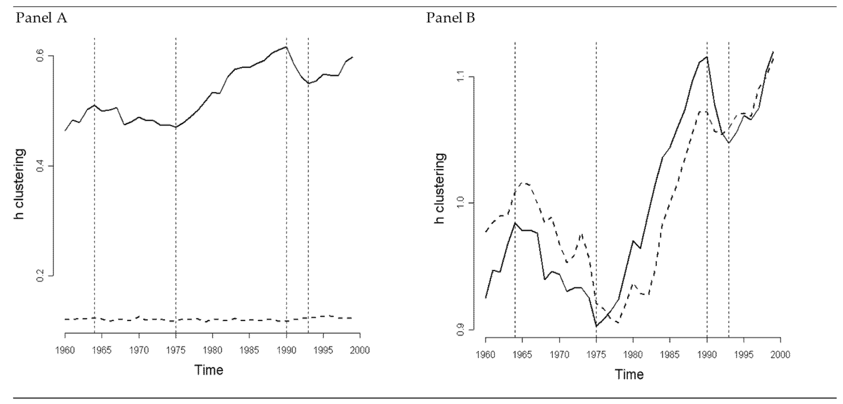
Figure 6 reports the results for the world economies. As above, in panel A the solid line reports the h-clustering index and the dashed line displays the optimal bandwidth as defined in Scheather and Jones (1991) [30]. The solid line in Panel B reports the h-convergence index, together with the plot of the variance, which is represented by the dashed line.
The results reported in panel A suggest that the optimal smoothing parameter is always smaller than the critical bandwidth for unimodality. This evidence suggests that unimodality is always rejected. This supports the evidence in Quah (1997) [11] that the distribution of incomes per capita is bimodal, as there exists two clusters in the distribution. Moreover, in 1960 the index is lower than in 1999. In the period spanning these two years, the two groups of countries experienced a process of divergence.
However, in sharp contrast with the only persistence concussion reported in Quah (1997) [11], we found some non-random fluctuations in the distribution of incomes. The sample period under analysis may be divided into three sub-periods—namely 1960–1964, 1964–1975, and 1975–1999. In the first and the last of sample these periods, economies experienced a club convergence process. The evidence also suggests that in the 1975–1999 period economies experienced a period of convergence from 1990 to 1993 but that divergence resumed afterward. By contrast, in the period from 1964 to 1975 the evidence is against the CCH. This is consistent with the evidence provided by Bianchi (1997) [12] that fails to reject unimodality throughout the 1970s.
Panel B supports the existence of the same sub-periods. More specifically, there exists a process of absolute convergence over the period from 1964 to 1975. From 1975 to 1990, the sample experienced a strong divergence process; the evidence suggests that this process accelerates throughout the 1980s.

5. Concluding Remarks

This paper contributes to the growth and convergence debate in three respects. Its first contribution lies in the approach that should be taken when studying convergence at the regional level. Contrary to the conventional wisdom, the ACH and the CCH should not be taken as competing hypotheses in empirical studies. Indeed, because they often involve similar economies or economies which are geographically closer to each other, club convergence processes are likely to be faster than the absolute convergence patterns that involve all the economies. In turn, this suggests that evidence in favor of the latter may or may be not taken as evidence against the former. Our empirical results for the Italian case support this argument.
Its second contribution lies in a procedure that helps to study the ACH and the CCH separately. We suggest studying the evolution of an index of clustering to assess the CCH—namely, the critical bandwidth for unimodality—and to correct this metric using the mean of the sample variance, as a test of the ACH. The procedure we propose allows for the identification of years where the convergence process shows a pattern reversal—from convergence to divergence or vice versa. This information, in principle, can help in studying why samples diverge or converge. It is indeed reasonable to study whether the occurrence of events preceding these years had an influence on the subsequent convergence dynamics—both clustering processes and convergence dynamics.
We apply the procedure we propose to four samples of economies. Our procedure provides new evidence for the samples of economies under analysis—which is our third contribution to the literature. Our results suggest that Italian regions converge until 1971, instead of 1975 as suggested by previous literature. This is confirmed by the sample of provinces, the analysis of which also shows that some provinces moved from the rich cluster to the poor cluster in 1991. EU regions show convergence until 1985, and divergence thereafter, in a process of general convergence. Finally, we find that, in an overall process of divergence and clustering, world countries experienced a convergence sub-period that ends in 1975.
The main limitation of our analysis is the absence of a reliable inference framework. How to obtain an inference framework in the non-parametric setting is not obvious, and is the subject of discussion among researchers. There are three approaches that may potentially be followed. Firstly, we could assume a known distribution for the clustering index. Secondly, we could use a Monte Carlo simulation for the cross-sectional distributions and recover the parameters of interest from all the estimates so as to have the empirical distribution of the statistics of interest. Finally, we could use perturbation techniques for the time series of the relative GDP per capita of each observation. Once the preferred approach is decided upon, we could recover some moments of this distribution to build an appropriate confidence interval. Each of these approaches have pros and cons, and we leave these questions for further research.

Funding

This research received no external funding.

Data Availability Statement

Data are available upon request from the authors.

Conflicts of Interest

The authors declare no conflicts of interest. The funders had no role in the design of the study; in the collection, analyses, or interpretation of data; in the writing of the manuscript; or in the decision to publish the results.

References

  1. Gonzalez-Paramo, J.M.; Martinez-Lopez, D. Convergence Across Spanish Regions: New Evidence on the Effect of Public Investment. R. Reg. Stud. 2003, 33, 184–205. [Google Scholar] [CrossRef]
  2. Lima, L.R.; Hostalacio, H.; Reis Gomes, F.A. Empirical Evidence on Convergence Across Brazilian States. Rev. Braz. Econ. 2010, 64, 135–160. [Google Scholar]
  3. Kholodilin, K.A.; Oshchepkov, A.; Siliverstovs, B. The Russian Regional Convergence. East. Eur. Econ. 2012, 50, 5–26. [Google Scholar] [CrossRef]
  4. Goeche, H.; Huter, M. Regional Convergence in Europe. Intereconomics 2016, 11, 165–171. [Google Scholar] [CrossRef]
  5. Puente, S. Regional Convergence in Spain: 1980-2015. Econ. Bull. 2017, 21, 1–7. [Google Scholar]
  6. Eichergreen, B. Convergence and Divergence in the EU: Lessons from Italy. Intereconomics 2019, 54, 31–34. [Google Scholar] [CrossRef]
  7. Lehmann, H.; Oshchepkov, A.Y.; Silvagni, M.G. Regional Convergence in Russia: Estimating a Neoclassical Growth Model; Higher School of Economics Research Paper No. WP BRP 232/EC/2020; SSRN: Rochester, NY, USA, 2020; pp. 1–48. [Google Scholar]
  8. Savoia, F. Income Inequality Convergence Across EU Regions; LIS Working Paper Series No. 760; Luxembourg Income Study (LIS): Luxembourg, 2020; pp. 1–40. [Google Scholar]
  9. Ram, R. Income convergence across the U.S. states: Further evidence from new recent data. J. Econ. Finan. 2021, 45, 372–380. [Google Scholar] [CrossRef]
  10. Acemoglu, D. Introduction to Modern Economic Growth; Princeton University Press: Princeton, NY, USA, 2009. [Google Scholar]
  11. Quah, D. Empirics for Growth and Distribution: Stratification, Polarization and Convergence Clubs. J. Econ. Gr. 1997, 2, 27–59. [Google Scholar] [CrossRef]
  12. Bianchi, M. Testing for convergence: Evidence from nonparametric multimodality test. J. Appl. Economet. 1997, 12, 393–409. [Google Scholar] [CrossRef]
  13. Fanti, L.; Pereira, M.C.; Virgillito, M.E. The North-South divide: Sources of divergence, policies for convergence. J. Pol. Mod. 2023, 45, 405–429. [Google Scholar] [CrossRef]
  14. Silverman, B.W. Using Kernel Density to Investigate Multimodality. J. Roy. Stat. Soc. 1981, 43, 97–99. [Google Scholar] [CrossRef]
  15. Terrasi, M. Convergence and Divergence Across Italian Regions. An. Reg. Sc. 1999, 33, 491–510. [Google Scholar] [CrossRef]
  16. Calcagnini, G.; Perugini, F. Income distribution dynamics among Italian provinces. The role of Bank Foundations. Appl. Econ. 2019, 29, 3198–3211. [Google Scholar] [CrossRef]
  17. Quah, D. Empirical Cross-Section Dynamics in Economic Growth. Eur. Econ. R. 1993, 37, 426–434. [Google Scholar] [CrossRef]
  18. Barro, R.J.; Sala-i-Martin, X. Convergence across States and Regions. Brook. Pap. Econ. Act. 1991, 1, 1107–1182. [Google Scholar] [CrossRef]
  19. Canova, F.; Marcet, A. The Poor Stay Poor: Non-Convergence across Countries and Regions; Discussion Paper No. 1265; Centre for Economic Policy Research (CEPR): London, UK, 1995. [Google Scholar]
  20. Bernard, A.; Durlauf, S.N. Convergence in International Output. J. Appl. Economet. 1995, 10, 97–108. [Google Scholar] [CrossRef]
  21. Quah, D. Twin Peaks: Growth and Convergence in Models of Distribution Dynamics. Econ. J. 1996, 106, 1045–1055. [Google Scholar] [CrossRef]
  22. Kremer, M.; Willis, J.; Yu, Y. Converging to Convergence. BFI WP 2021, 1–50. [Google Scholar]
  23. Patel, D.; Sandefur, J. Subramanian, A. The new era of unconditional convergence. J. Dev. Econ. 2021, 152, 1–18. [Google Scholar] [CrossRef]
  24. Rosenblatt, M. Remarks on Some Nonparametric Estimates of a Density Function. An. Math. Stat. 1956, 27, 832–837. [Google Scholar] [CrossRef]
  25. Caggiano, G.; Leonida, L. International output convergence: Evidence from an autocorrelation function approach. J. Appl. Economet. 2009, 24, 139–162. [Google Scholar] [CrossRef]
  26. Caggiano, G.; Leonida, L. Multimodality in the distribution of GDP and the absolute convergence hypothesis. Emp. Econ. 2013, 44, 1204–1215. [Google Scholar] [CrossRef]
  27. Leonida, L. What Have We Not Learned from the Convergence Debate? Mathematics 2023, 11, 2119. [Google Scholar] [CrossRef]
  28. Marron, J.S.; Schmitz, H.P. Simultaneous density estimation of several income distributions. Econ. Theory 1992, 8, 476–488. [Google Scholar] [CrossRef]
  29. Silverman, B.W. Density Estimation for Statistics and Data Analysis; Chapman and Hall: London, UK, 1986. [Google Scholar]
  30. Sheather, S.J.; Jones, M.C. A reliable data-based bandwidth selection method for kernel density estimation. J. Roy. Statist. Sot. Ser. E 1991, 53, 683–690. [Google Scholar] [CrossRef]
  31. Mauro, L.; Podrecca, E. The Case of Italian Regions: Convergence or Dualism. Econ. Not. 1994, 447–472. [Google Scholar]
  32. Paci, R.; Saba, A. The Empirics of Regional Economic Growth in Italy, 1951–1993. Riv. Inter. Sci. Econ. Comm. 1998, 5, 513–542. [Google Scholar]
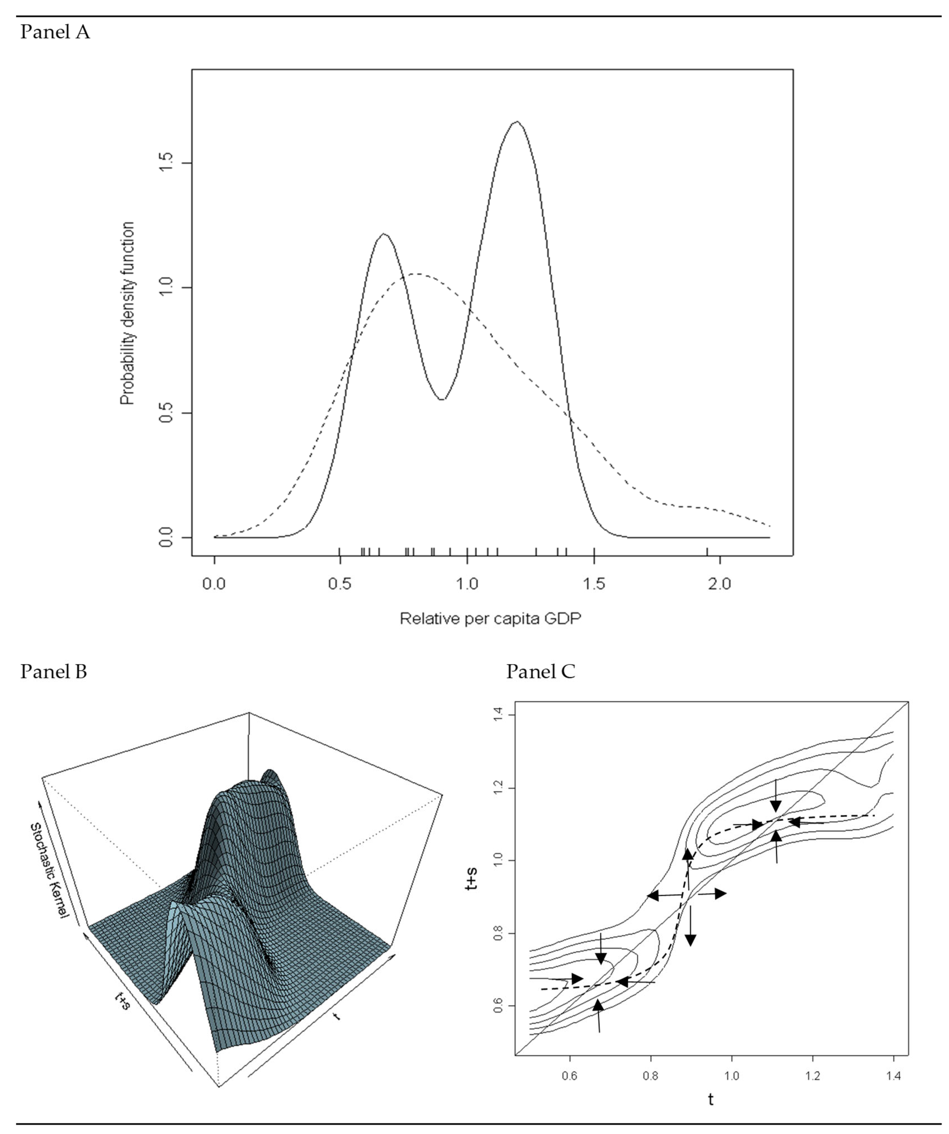
Figure 1. Analysis of the distribution of income per capita across Italian regions: 1951 to 1999. Panel (A) reports the estimate of the distribution of income per capita under the hypothesis that data are normally distributed. Solid line stands for 1951; dashed line stands for 1999. Panel (B) reports the stochastic kernel estimated for transitions of twenty years (i.e., s = 20) between 1951 and 1999. Vectors t and t + s consist of 1248 observations of relative income per capita. The estimate is performed by means of the Gaussian Kernel under the hypothesis that data are normally distributed. Panel (C) reports the contours plot of the estimate for fixed levels of probability, where p = 0.20, 0.25, 0.30, 0.35, 0.40, respectively.
Mathematics 12 00256 g001
Figure 2. Analysis of the distribution of GPD per capita across Italian regions: 1951 to 1971. Panel (A) reports the estimate of the distribution of income per capita obtained under the hypothesis that data are normally distributed. Solid line stands for 1971; dashed line stands for 1951. Panel (B) reports the smoothed differences between 1971 and 1951. Panel (C) reports the stochastic kernel estimated for transitions of twenty years (i.e., s = 20) between 1951 and 1971 for Italian regions. Vectors t and t + s consist of 600 observations of relative income per capita. The estimate is performed by means of the Gaussian Kernel under the hypothesis that data are normally distributed. Panel (D) reports the contours plot of the estimate for fixed levels of probability, where p=0.20, 0.25, 0.30, 0.35, 0.40, respectively.
Mathematics 12 00256 g002
Figure 3. h-Convergence Analysis for Italian Regions. In panel (A) the solid line and the dashed line represent the h-clustering metric and the series that builds upon the Scheather-Jones bandwidth series, respectively. In panel (B) the solid line and the dashed line represent the h-convergence index and the metric that builds upon the variance, respectively. In panels (C,D) we report the analysis after taking natural logarithms of income per capita.
Mathematics 12 00256 g003
Figure 4. h-Convergence Analysis for Italian Provinces. In panel (A) the full line and the dashed line represent the h-clustering metric and the series that builds upon the Scheather-Jones bandwidth series, respectively. In panel (B) the full line and the dashed line represent the h-convergence index and the metric that builds upon the variance, respectively.
Mathematics 12 00256 g004
Figure 5. h-Convergence Analysis for EU Regions. In panel (A) the full line and the dashed line represent the h-clustering metric and the series that builds upon the Scheather-Jones bandwidth series, respectively. In panel (B) the full line and the dashed line represent the h-convergence index and the metric that builds upon the variance, respectively.
Mathematics 12 00256 g005
Figure 6. h-Convergence Analysis for World Economies. In panel (A) the full line and the dashed line represent the h-clustering metric and the series that builds upon the Scheather-Jones bandwidth series, respectively. In panel (B) the full line and the dashed line represent the h-convergence index and the metric that builds upon the variance, respectively.
Mathematics 12 00256 g006
Disclaimer/Publisher’s Note: The statements, opinions and data contained in all publications are solely those of the individual author(s) and contributor(s) and not of MDPI and/or the editor(s). MDPI and/or the editor(s) disclaim responsibility for any injury to people or property resulting from any ideas, methods, instructions or products referred to in the content.