Abstract
In order to provide urban freight vehicles with navigation routes that better align with their travel preferences, it is necessary to analyze the patterns and characteristics of their route choices. This paper focuses on freight vehicles traveling within the city and examines their route selection behavior. Through an analysis of the GPS data collected from freight truck journeys in Changchun, China, this study outlines the characteristics of freight vehicle travel within the city. Variables that may influence their route selection behavior are defined as feature factors. The study employs the DBSCAN algorithm to identify the hotspots in origin–destination pairs for freight truck travel in Changchun. It also utilizes Breadth First Search Link Elimination to generate a set of route choices and constructs route selection behavior models based on Multinomial Logit and Path Size Logit. Based on the research findings, during navigation within the city road network, these vehicles exhibit a preference for side roads, a tendency to favor right turns at intersections, and a propensity to choose routes with lower duplication compared to alternative options. The study’s conclusions offer theoretical support for guiding urban freight vehicle routes and planning and managing freight traffic within the city.
MSC:
62C99
1. Introduction
The study of route selection behavior has been ongoing since the last century and has always been a crucial component of transportation research. Research on vehicle route selection behavior can help people understand drivers’ route preferences and travel characteristics, enabling route guidance and traffic allocation for traveling vehicles, ultimately improving the operational efficiency of transportation systems [1].
Before the widespread adoption of GPS positioning technology, collecting objectively accurate vehicle travel data has always been a challenge in modeling route selection behavior. Many scholars have obtained driver decision processes by conducting interviews or administering preference surveys [2,3], such as Abdel-Aty et al., who collected binary choice sets from commuters under various travel scenarios using phone interviews and mail surveys [4]. However, as discussed by Bierlaire and Frejinger, collecting vehicle travel data from drivers’ recollections is labor-intensive, yields limited data, and cannot guarantee the data accuracy [5]. Compared to traditional survey data, vehicle GPS trajectory data may not provide personal information such as on the driver’s age, gender, and education. However, it can offer more comprehensive and precise geographic information, and facilitate easier large-scale data acquisition. This provides comprehensive data support for modeling route selection behavior. This paper utilizes extensive GPS data to analyze the spatiotemporal characteristics and patterns of freight vehicle travel within urban areas. It constructs a PSL model that includes multi-level variables such as travel time, the number of intersections, route detours, and route selection proportions. To ensure the accuracy of the route selection model results, the MNL model is used for comparison. The study analyzes the impact of various feature variables on freight truck route selection behavior based on the parameter calibration results of both models.
The main novelty of this study lies in the analysis of the route selection behavior of freight vehicles on urban roads. Previous research on route selection behavior has mainly focused on taxis, commuting vehicles, and long-distance freight vehicles, paying less attention to the travel activities of freight vehicles within the urban road network. This oversight neglects the impact of freight vehicles on urban traffic. In this study, we specifically analyze the route selection behavior of freight vehicles in urban road networks, complementing the modeling of the urban freight vehicle route selection behavior using GPS data. Furthermore, based on a large-scale GPS dataset, this study summarizes the travel patterns and characteristics of freight vehicles in urban road networks from both temporal and spatial perspectives. This differs from other relevant studies on truck route selection behavior.
The other sections of the study are structured as follows: Section 2 presents a literature review on route choice behavior, Section 3 discusses the processing of the initial dataset, Section 4 introduces the models and methods used in the study, Section 5 delves into the model calibration results, and Section 6 summarizes the research.
2. Literature Review
2.1. Current Status of Route Choice Behavior Modeling Research
The study of route choice behavior can be broadly categorized into two main types. One type is based on theoretical frameworks such as prospect theory, fuzzy logic theory, game theory, etc. The other type involves studying route choice behavior based on various Logit-type discrete choice models.
- (1)
- Research on Route Choice Behavior Based on Theoretical Frameworks
Prospect theory is built on the foundation of bounded rationality theory, aiming to explore decision-makers’ choice behavior in the face of different gains or losses in situations with unknown influencing factors [6]. It was later proven to accurately reflect travelers’ attitudes when facing unknown risks and has been widely applied to route choice behavior in various uncertain environments [7]. Gao et al. studied the route choice behavior of different types of travelers under given information using the longest, shortest, and average travel times as reference points [8].
The application of fuzzy logic theory in modeling route choice behavior primarily focuses on fuzzy rules and fuzzy ranking. Teodorovic D was the first to apply fuzzy theory to complex route choice problems, using fuzzy reasoning techniques to solve dual-layer route choice problems [9]. Peeta and Yu used fuzzy rules to simulate en-route driver behavior under real-time information [10].
Game theory is an important mathematical theory and method for studying phenomena of a competitive or strategic nature. It aims to explore the interactions between different incentive structures. Wardrop first attempted to introduce game theory into the field of transportation and proposed the first and second principles of traffic network equilibrium. Since then, the application of game theory in the field of transportation has gradually become widespread [11].
- (2)
- Research on Route Choice Behavior Based on Discrete Choice Models
McFadden and others, based on random utility theory, assuming that the random utility term follows a Gumbel distribution, proposed the Multinomial Logit (MNL) model [12]. The MNL model has been widely applied due to its simple structure and excellent performance. However, the MNL model has its limitations, as its assumption about the random utility term prevents it from considering the similarity between alternative routes.
To address the shortcomings of the MNL model, many scholars have proposed various improved models. Ben-Akiva, by introducing a correction term into the basis of the traditional MNL model to reduce the utility overlap of alternative paths and thus avoid the independence of irrelevant alternatives (IIA) flaw, proposed the Path Size Logit (PSL) model [13]. Some scholars, based on the Generalized Extreme Value (GEV) theory, proposed improved models that reflected the differences between different paths in the form of random error terms, forming a nested structure. Examples include Chu’s Paired Combinatorial Logit (PCL) model [14], Vovsha’s Cross Nested Logit (CNL) model [15], and Wen’s Generalized Nested Logit (GNL) model [16]. Additionally, some scholars combined Gumbel distribution and normal distribution, proposing the Mixed-Logit (ML) model [17].
Compared to theoretical models, discrete choice models can more accurately analyze the impact of different factors on travelers’ route choice behavior by simulating their route choice behavior based on actual transportation data. Currently, the modeling process of route choice behavior mainly relies on various discrete Logit models, among which MNL, CL, PSL, GNL, CNL, PCL, and ML are the most significant types of discrete Logit models in route choice behavior research.
2.2. Current Status of Vehicle Route Choice Behavior Research
GPS devices are widely used in private and public vehicles, and taxi and commuter vehicles have become primary subjects of route selection behavior research. For example, Tang and others analyzed the multi-day route selection behavior of travelers using GPS data from the Minneapolis–St. Paul metropolitan area. The study found that most travelers use the same route for their daily commutes, and different types of travelers exhibit significant differences in their route selection attributes [18]. Sun and others, based on taxi GPS data, analyzed the factors that may influence drivers’ route selection behavior. They found that travel distance, travel time, and road preferences significantly impact drivers’ route choices. They proposed a new route prediction model with constraints based on the shortest path length and the fastest path travel time, validating it using GPS data from Shenzhen’s taxi fleet [19].
Nowadays, research on route selection behavior is rapidly evolving and becoming more diverse. Its scope of study is no longer limited to just taxis and commuter vehicles. Some scholars (Hood, Broach) have begun to investigate the route selection behavior characteristics of bicycles [20,21]. Additionally, urban freight transportation demands are on the rise, and the increasing number of freight vehicles exacerbates urban traffic safety and pollution issues. Thus, there is a growing focus on the patterns and characteristics of freight vehicle travel, leading to an increase in research related to the route selection behavior of freight vehicles [22,23]. For instance, Feng and Arentze established a model for freight truck route selection behavior, revealing that long-distance truck drivers pay more attention to road congestion levels and are highly sensitive to road tolls [24]. Hess and colleagues applied the error component Logit model to analyze heavy truck route choices across the entire road network in England using GPS data, showcasing the potential of using discrete choice models to analyze route choices in the extensive network of freight vehicles [25]. Oka Hideki and others used freight truck GPS data to analyze and predict changes in the travel patterns of freight vehicles in the Tokyo metropolitan area. They developed a route selection model based on the concept of the maximum path overlap ratio. Finally, they simulated and predicted the changes in freight traffic flow patterns under different policy scenarios, proposing traffic policy recommendations to alleviate urban traffic congestion and improve freight efficiency [26].
Fu Yanhong and others analyzed the spatiotemporal characteristics of truck travel based on truck GPS data. In addition, they compared the sample data with actual situations to verify the reliability of this method for analyzing truck operation characteristics based on GPS data [27]. Jun Huang and others discussed a large-scale truck trajectory dataset, analyzing the spatiotemporal characteristics of truck travel from various perspectives, including departure time, travel distance, and working hours. They used the LCSS method to calibrate the similarity of all the journeys in the data and conducted cluster analysis. The conclusion drawn was that the most frequently chosen route is the shortest path between the initial node and final node. Truck drivers may choose a longer route because they need to load and unload goods in intermediate cities along that route [28].
Currently, most of the research on freight vehicle route selection behavior focuses on long-distance travel between provinces. There is still relatively limited and insufficient research on the route selection behavior and travel distribution patterns of freight vehicles within cities. This gap in knowledge hinders the provision of scientifically sound guidance for managing urban freight vehicles.
2.3. Current Status of Route Choice Set Research
When calibrating route choice models, the size and composition of the choice set are crucial, as they can strongly influence the model estimates. Incorrect choice sets can lead to biased parameter estimates and choice probabilities [29,30].
Currently, the methods for constructing route choice sets mainly include shortest path algorithms, finite enumeration methods, and probability analysis methods. Ben-Akiva initially employed the label method to construct route choice sets. By comparing different combinations of labels, it was discovered that among all label categories, time and distance had the greatest impact on generating the actual chosen paths of vehicles. Considering time and distance could generate approximately 70% of the selected paths, while the influence of signal light quantity on generating the actual chosen paths of the vehicles was minimal [31].
Prato and Bekhor constructed a new branch-and-bound method to generate route choice sets, focusing on commuting travel. They compared this method with the label method, segment elimination method, segment penalty method, and simulation method [32]. Piet H. L. Bovy summarized the research related to route choice sets, and discussed various uses of route choice sets and the significance of these uses for practical modeling. The research found that distinguishing between the actual vehicle travel paths and the paths in the route choice set is advantageous for constructing route choice models [33].
Frejinger et al. developed a random walk algorithm. The idea behind this algorithm is to start from the initial node and, based on the shortest path distance between the link length and its final node, select the next link (based on the Kumaraswamy distribution). This operation is repeated until reaching the target node [34].
The aforementioned methods for constructing route choice sets are relatively mature; however, most of these methods were developed for low-resolution networks, and do not address the challenges posed by high-precision large-scale traffic networks. Rieser Schüssler proposed the Breadth First Search Link Elimination (BFS-LE) algorithm [35]. The BFS-LE algorithm is specifically designed to construct choice sets for large-scale, high-precision road networks.
The literature review above indicates that significant work has been undertaken in the field of route choice behavior. However, there is a need for further research on truck route choice behavior. This study focuses on the route selection behavior and travel characteristics of freight vehicles within urban road networks, a specific subset that requires additional investigation.
3. Data
This study selected Changchun City as the research area and obtained road network data from the OpenStreetMap (OSM) open-source mapping platform (Figure 1). The dataset comprises 14,831 road segments and 29,748 nodes, encompassing all the road segments relevant to vehicle travel. The GPS trajectory data for small and medium-sized trucks in Changchun City from May to September 2020 were acquired as the foundational dataset from the Intelligent Transportation Open Platform. The cargo types carried by the trucks in the dataset are primarily related to production and service materials. The source data consist of 24,638 files, with each record containing seven fields: longitude, latitude, time, true north direction angle, distance, speed, and altitude.
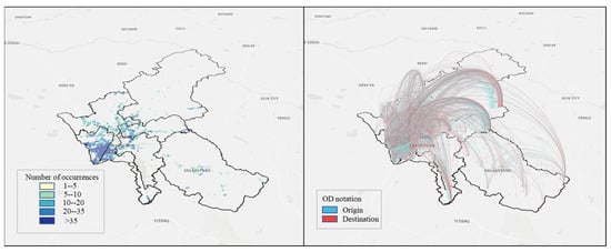
Figure 1.
Spatial distribution of freight vehicle travel in Changchun City.
3.1. Initial Dataset Processing
The study performs the following cleaning on the initial GPS dataset:
- Cleaning of Stationary Vehicle Data: Eliminating GPS data related to stationary vehicles from the dataset.
- Interstate Freight Data Cleaning: Since this study focuses on the route selection behavior within the city, GPS data points that fall outside the administrative boundaries of Changchun City were removed from the dataset.
- Cleaning of Abnormal Time Frequency Data: Cleaning GPS data points that are repeatedly recorded at abnormal time frequencies. For example, in Table 1, three data points within the dashed box exhibit identical time series, latitude, and longitude features, yet they are recorded multiple times. Such data points are considered to have abnormal time frequencies.
 Table 1. Example of abnormal time frequency data.
According to the research objectives and requirements of the study, the following preprocessing steps were applied to the base road network:
- Road Segment Selection: Excluding non-motorized vehicle-specific road segments, such as footways, steps, and pedestrian paths, from the original road network data. These types of roads are not relevant to the route selection behavior of freight vehicles. Road types were consolidated into five categories: highways, expressways, main roads, secondary roads, and local roads.
- Road Segment Division: Dividing road segments at intersections to allow vehicles to make turns at these points, simulating the real-world turning topology at road intersections. Special segments in the road network, such as bridges, expressways, and highways with significant elevation differences from regular ground-level roads, were separately processed.
- Projection Transformation: Transforming the road network from the WGS84 geographic coordinate system into the Xian_1980_3_Degree_GK_CM_120E plane coordinate system and calculating the lengths of the road segments.
- Extracting Road Network Node and Segment Information: Using ArcGIS to construct a network dataset for the road network, extracting nodes for all road segments, and generating node identifiers. The “Connect” tool was employed to associate each road segment with its respective nodes, obtaining information such as the initial node and final node, lengths, and identifiers for each road segment. Table 2 presents the tabular format of the extracted road segment information.
Table 2. Road segment information table.
- Building a Road Network Model: Using Python to read the node identifiers, lengths, and segment identifiers for all road segments in the road network, and utilizing the free-flow travel time for each road segment as the weight, the road network model is constructed using the Networkx library.
3.2. Map Matching
GPS location points are often affected by various factors such as the GPS device signal quality, performance, and environmental interference, causing them to deviate from their actual positions. In this study, a Hidden Markov Model (HMM) is used for map matching of the GPS location points. The HMM treats the latitude and longitude of GPS location points as observable variables, while the true location of the traveling vehicle is treated as a hidden state variable. By calculating the measurement probabilities and state transition probabilities for each candidate point, the HMM method predicts the true location of the traveling vehicle based on probability.
Figure 2 displays a portion of the trajectory data after map matching using the HMM. After map matching, the GPS location points are repositioned onto the corresponding road segments, forming a complete travel path. Using this path, we can further calculate information about the path, such as the lengths of various road segments, the number of intersections passed through, and the count of left or right turns taken.
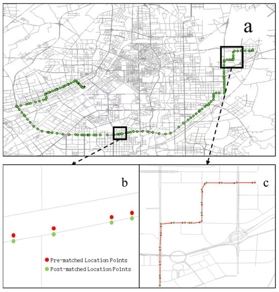
Figure 2.
Partial map matching results. (a) Full path after matching. (b) Pre-matched and post-matched location points. (c) Partial path after matching.
3.3. Clustering Trajectory Data into OD Pairs Using the DBSCAN Algorithm
The dataset used in this study contains over 20,000 GPS data points for truck travel, resulting in a substantial number of OD pairs distributed across various areas within Changchun City. This posed a significant challenge in creating sets of route choices between OD points for subsequent analysis. Therefore, this research employed the DBSCAN clustering algorithm to cluster the OD pairs from the truck trajectory data. This approach helps identify hotspots for urban truck travel OD pairs and effectively filters out the trajectory data from low-density point areas.
Firstly, clustering is applied to the starting points of truck trips. The value of the clustering neighborhood radius (Eps) is determined using the K-distance curve. The minimum density threshold (MinPts) that provides stable and effective clustering results is determined using an iterative approach. According to Figure 3, the Eps value is determined to be 0.00134811, and the MinPts value is 530. After clustering the starting points, trajectory data labeled as noise points are removed from the clustering results. Subsequently, clustering is performed again on the endpoints of the remaining trips. Using the same method as described above, the Eps value for this clustering is determined to be 0.001321605, with a MinPts value of 400.
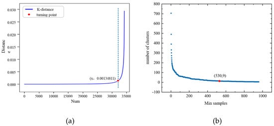
Figure 3.
K-distance curve and Minimum density threshold-cluster number curve. (a) K-distance curve. (b) Minimum density threshold-cluster number curve.
Figure 4 depicts the distribution of the clustering results. In the end, a total of nine hotspots were obtained for the starting points of truck trips, along with six hotspots for the endpoints of truck trips. These hotspots for the initial node and final node of trips form a total of 54 OD pairs, with freight truck travel journeys occurring in 27 of these OD pairs. These 27 OD pairs are considered the hotspots for truck travel. In total, 7713 truck trajectory data were retained for subsequent research on urban truck route selection behavior. This ensures that among the selected trajectory data, both the starting and ending points of truck trips belong to the clustered hotspots.
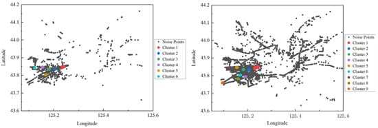
Figure 4.
Clustering results.
4. Analysis Methodology
4.1. Constructing the Route Choice Set
In the context of traveler route choice behavior research, the choice set refers to the collection of travel paths that drivers may choose between the initial node and final node of a trip. The road network dataset chosen for this study is large in scale and high in precision. Therefore, the Breadth First Search (BFS) algorithm, suitable for generating large-scale road network route choice sets, was selected. Compared to other algorithms for building choice sets, the BFS-LE algorithm ensures the diversity of the generated candidate paths, and is faster in terms of its computation speed [36].
The BFS-LE algorithm is based on repeatedly searching for the minimum-cost path. Figure 5 illustrates the principle of the BFS-LE algorithm. This algorithm uses a tree-like structure to generate new networks by progressively removing road segments, using the free-flow travel time of road segments as the cost function to calculate the travel cost of each path. The initial network consists of the complete road network, which is the 0th level of the tree. Starting from the root node of the tree (the initial network), it searches for the minimum-cost path from the initial node to the destination in the current network, removing road segments one by one to create a new road sub-network. Each newly generated sub-network becomes a node in the tree, forming the first level. It then re-searches for the minimum-cost path between all OD pairs of the first-level nodes, removing road segments, one by one, to obtain the second-level nodes. This process is repeated, and the minimum-cost paths from all levels of networks generated by the algorithm are included in the choice set. The algorithm continues until no more feasible paths can be found or until it reaches the predetermined time threshold and path quantity for constructing the choice set.
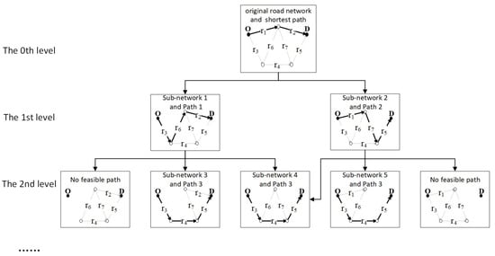
Figure 5.
BFS-LE algorithm principle.
To enhance the computational efficiency of the algorithm and improve the quality of the generated choice set, this study introduced several rules into the initial BFS-LE algorithm:
- (1)
- To prevent the algorithm from terminating prematurely due to road segment elimination, a new rule is added to the BFS-LE algorithm: the minimum cost search will start from the next node that is connected to at least two road segments in the travel path.
- (2)
- To ensure the uniqueness of each path in the choice set, the study uses a common factor proposed by Cascetta et al. [37] to assess the similarity between paths, setting a critical value of 0.95 for the common factor. Only when the common factor between the newly generated path in the BFS-LE algorithm and the previously generated path is less than or equal to 0.95 will this path be included in the choice set. The formula for calculating the common factor is as follows:In the formula, and represent the lengths of path i and path j, while represents the length of the overlapping section between the two paths.
- (3)
- In a complex urban road network, there may be hundreds of feasible paths between given OD pairs. To prevent an excessively long running times and improve the algorithm efficiency, the algorithm has set termination conditions: it is specified that the algorithm will end when the number of paths generated between OD pairs exceeds 15 or when the algorithm runs for more than 60 min.
4.2. Path Choice Model
4.2.1. Model Feature Variables
The spatiotemporal characteristics of freight vehicle travel are essential for analyzing the behavior of large trucks [38]. In this section, we will use the driving information of freight trucks to analyze the travel characteristics of urban freight vehicles from both temporal and spatial perspectives. We will summarize the regularities and, based on the analysis results, identify the factors that may influence the route selection behavior of truck drivers as feature variables in the path choice model (Figure 6).
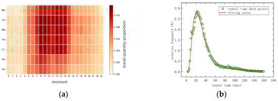
Figure 6.
Travel time distribution characteristics. (a) Frequency distribution of travel time of urban freight vehicles. (b)Daily distribution statistics for the number of truck trips.
Based on Figure 6, the statistical chart of urban freight vehicle travel time distribution, the following conclusions were drawn
- (1)
- Urban freight truck travel is primarily concentrated on weekdays, with significantly higher travel volumes from Tuesday to Friday compared to the other days of the week. The peak travel periods for freight vehicles in Changchun are from 8:00 to 10:00 and 12:00 to 14:00 daily, with most transport times avoiding the peak commuting hours in the morning and evening within the city.
- (2)
- Urban freight vehicle travel is predominantly short-distance, with the majority of travel times being within 60 min. The relative frequency of travel times for urban freight trucks approximately follows a log-normal distribution, with the highest relative frequency observed at a travel time of 21 min.
Based on the statistical chart of the urban freight vehicle travel path spatial characteristics in Figure 7, the following conclusions can be drawn:
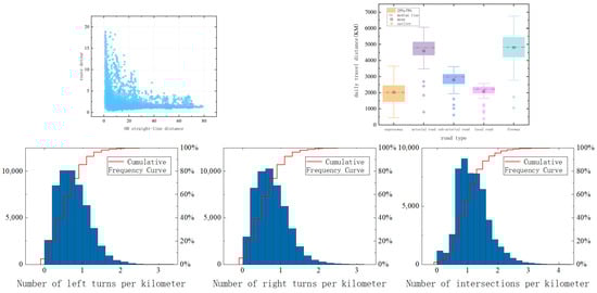
Figure 7.
Travel path spatial characteristics.
- (1)
- As the OD distance increases, the detour degree of most truck travel paths decreases, and the dispersion of data points gradually decreases. This indicates that as the travel distance increases, truck drivers are less willing to choose detours, and more drivers prefer routes with lower detour degrees.
- (2)
- Urban freight vehicles travel the longest distance on expressways on average each day, but the daily travel distance data on expressways and highways are less concentrated in the 25th percentile than the 75th percentile range, and have relatively high fluctuations in the upper and lower limits. Therefore, arterial roads, sub-arterial roads, and local roads are the main routes for most freight vehicles within the city.
- (3)
- The distribution of the number of left and right turns per kilometer in the travel paths of urban freight vehicles is similar. Most freight vehicles pass an average of 1 intersection per kilometer and make approximately 0.6 left/right turns per kilometer on city roads.
Based on the above analysis, the factors that may influence the path selection behavior of truck drivers (travel time, detour degree, left/right turn/intersection count, the proportion of different road types) are considered the feature variables for the urban freight vehicle path selection model (Table 3).
Table 3.
Feature variables for truck path selection model.
4.2.2. Model Construction
When analyzing the discrete choice behavior of decision-makers, building a Logit model is the most common research approach. The MNL model is a popular type of Logit model known for its simple structure, versatility, and high computational efficiency, making it a frequent choice for modeling discrete choice behavior.
The MNL model is based on the random utility theory, which posits that decision-makers tend to select options with higher utility. The utility for decision-makers to choose option can be expressed as:
In the equation, represents the fixed utility of the decision-maker choosing option , and represents the random utility for the decision-maker choosing option .
The Logit model assumes that the random utility terms are mutually independent and follow a uniform Gumbel distribution. The distribution parameter with can be represented by the distribution function :
As is mutually independent, the joint distribution function of can be represented as:
At this point, according to utility maximization theory, the probability of the decision-maker choosing option can be written in the following form:
In this equation, represents the set of options the decision-maker can choose from.
While the traditional MNL model is classic, it has its limitations. The MNL model assumes the “independence of irrelevant alternatives” (IIA) characteristic when choosing any two categories in the reflected variables [39]. When the MNL model is applied to modeling route choice behavior, the IIA characteristic manifests as a lack of consideration of the similarity between alternative choices due to overlapping routes, which can impact the accuracy of the model calibration results.
In order to adapt discrete choice models to path selection problems, some models have started to explain the similarity between different alternative paths within the same road network [40]. The PSL model is an improvement over the MNL model when applied to route choice behavior research. It builds upon the MNL model by adding correction terms that capture the correlation between alternative route choices, thereby eliminating the influence of the IIA characteristic in route choice modeling. The PSL model offers strong interpretability and high computational efficiency. Compared to the MNL model, the PSL model reflects the proportion of road segments on a particular path in the entire set of path choices. It can address the accuracy issues in model calibration caused by the presence of overlapping road segments in different paths, providing results that better align with the actual probabilities of selecting overlapping paths. Additionally, the PSL model exhibits stronger explanatory power for travel path selection behaviors. Therefore, this study will use the PSL model to analyze the route choice behavior of urban freight vehicles. Additionally, to ensure the accuracy of the route choice model results, a traditional MNL model will also be constructed, and its calibration results will be used for comparative analysis.
The PSL (Path Size Logit) model, while maintaining the basic structure of the MNL (Multinomial Logit) model, introduces a PS (Path Size) correction term into the deterministic part of the utility function. This correction term captures the similarity between the chosen route and all the other alternative routes within the choice set. A PS value closer to 1 indicates that the chosen route has less overlap with other routes. The formula for the PSi correction term is as follows:
In this formula, PSi represents the correction term for route i. stands for the set of segments in route i. represents the length of segment . is the length of route i. is the set of all routes between OD points. is a binary variable that equals 1 if segment is on route l, and 0 otherwise.
Now, by incorporating the correction term into Formula (5), the final PSL model can be expressed as follows:
In this formula, represents the parameters to be estimated.
5. Results and Discussion
5.1. Parameter Calibration Results
We divided all the travel trajectory data into two parts, with 70% of the data (a total of 5405 entries) used to build the path choice model and 30% of the data (a total of 2308 entries) used to evaluate the models’ prediction accuracy. Based on the travel trajectory data, we constructed the path choice model and estimated the model parameters using the Biogeme package in Python (3.9). The final calibration results for the PSL model and the MNL model are shown in Table 4.
Table 4.
Comparison of parameter calibration results for different models.
5.2. Model Evaluation and Predictive Accuracy Test
5.2.1. Model Evaluation
After completing the parameter calibration of the path selection model, it is necessary to evaluate the models’ explanatory power and goodness of fit based on the calibration results to assess the ability of the models’ independent variables to explain the dependent variable and the models’ accuracy. We use p-values and Student’s t-values to evaluate the significance level of various variables in the models, use values to assess the models’ explanatory power, and use and Adj values to evaluate the models’ goodness of fit.
Student’s t-values refer to a test method used to examine whether the independent variables in a model have a significant impact on the dependent variable. p-values are the calculated significance levels based on actual statistical measures and are used to determine the significance of the results of a hypothesis test. From Table 4, it can be seen that the p-values for the explanatory variables in both the MNL and PSL models are less than 0.05, And the absolute values of Student’s t-values are all greater than 1.96. This suggests that with 95% confidence, the explanatory variables in the models are significantly associated with the path choice results. It can be considered that the selected models’ independent variables are reasonable and the independent variables have good statistical validity for calibrating the model parameters.
The value is defined as the difference in the log–likelihood between the null hypothesis model and the proposed model and is a test of whether the independent variables contained in the model are linearly related to the dependent variable’s log–odds. The formula for calculating the value is as follows:
In the formulas provided, represents the log–likelihood value of the null hypothesis model. represents the log–likelihood value of the assumed model.
By consulting a chi-square table, it can be determined that , , and the value in both the MNL and PS Logit models from Table 4 are all greater than 16.92. This indicates that the independent variables in the path selection models built in this study have a significant explanatory power for the dependent variable.
In order to evaluate the goodness of fit of the model, the likelihood ratio or McFadden’s R-squared is used, which is an index similar to R-squared in regression analysis. Expressed in mathematical form as the following formula, its symbol is defined as .
falls between 0 and 1, with values closer to 1 indicating higher model accuracy. In practice, a value between 0.2 and 0.4 is considered an indication of good model accuracy. In the calibration results, the likelihood ratios for the MNL and PSL models are 0.286 and 0.327, respectively. This suggests that both models exhibit good accuracy and can, to some extent, explain the path selection behavior of urban freight vehicles.
The Adjusted Rho-square coefficient takes into account the number of independent variables in the model and is a statistically adjusted measure of the Rho-square (coefficient of determination). It is also used to assess the goodness of fit of a regression model. In the calibration results, the adjusted for the MNL model and PSL model still falls within the range of 0.2 to 0.4.
5.2.2. Model Prediction Accuracy Test
This study evaluates the accuracy of model predictions by calculating the hit ratio of the path selection model. The calibrated model parameters are inserted into the already calibrated model. The probability of each alternative path in the path selection set for the OD pairs being selected is computed. A model’s hit ratio is calculated by comparing whether the actual path chosen by the driver matches the model’s predicted result. To assess the models’ prediction accuracy, 30% of the truck trajectory data (a total of 2308 trajectories) are used. The hit ratio results for the MNL model and the PSL model are shown in Table 5.
Table 5.
Hit ratio of path selection model predictions.
In a total of 2308 instances of path selection behavior, the PSL model correctly predicted the driver’s chosen path 1843 times, and the MNL model correctly predicted the driver’s chosen path 1618 times. The hit ratios for the two models are 79.85% and 70.10%, respectively. Both models achieved hit ratios exceeding 70%, indicating that the urban freight truck path selection models constructed in this study have a high level of prediction accuracy and are effective.
From the perspective of model evaluation and hit ratio testing, both models exhibited a good fit and prediction accuracy. This suggests that both models are capable of explaining the path selection behavior of urban freight vehicles to some extent. Furthermore, the PSL model outperformed the MNL model in terms of fit and prediction accuracy, indicating that, compared to the traditional MNL model, the PSL model provides a better fit and a more comprehensive explanation of the urban freight truck path selection behavior.
5.3. Result Analysis
Looking at the parameter estimation results of the models, it is clear that both models exhibit consistent positive or negative parameter values. This indicates that the effect of each influencing factor on the path selection behavior in both the MNL model and the PSL model is in the same direction. This further validates the rationality of the constructed path selection models.
Analyzing the p-values of each parameter in both models from Table 4, it is evident that each parameter has a significant impact on the models. This implies that both the MNL model and the PSL model contribute to explaining path selection behavior to a certain extent.
Analyzing the parameter estimation results of the MNL model and PSL model from Table 4, we can draw the following conclusions:
- (1)
- As anticipated, for all travelers, factors such as travel time, detour length, and the number of left turns/intersections in a path have a negative effect on path selection. In other words, travelers tend to prefer paths with shorter travel times, lower detour lengths, and fewer left turns/intersections. In the PSL model, the positive coefficient for Ln(PS) aligns with the basic principles of path selection models, indicating that the lower the overlap between path i and the other paths in the choice set, the more likely travelers are to select that path.
- (2)
- Unlike commuter and other vehicles’ travel behavior, when truck drivers choose travel paths on urban roads, the percentage of arterial roads and collector roads in the path negatively influences path selection. Meanwhile, the percentage of local roads positively influences path selection. Truck drivers tend to choose paths with lower percentages of arterial and collector roads and relatively higher percentages of local roads. This may be attributed to the fact that arterial roads often have more complex traffic conditions and congestion, leading to increased travel costs like travel time. Additionally, larger truck vehicles are more likely to cause congestion and traffic accidents in complex traffic environments, prompting truck drivers to prefer paths with a higher percentage of local roads.
- (3)
- Combining the urban freight vehicle travel characteristics with the model’s parameter estimation results, we can provide tailored path navigation using electronic mapping software to align with our travel preferences. For different distances of freight vehicles, targeted path induction can be carried out. Furthermore, for the hotspots of truck travel, it is essential to promote the construction of roads suitable for truck travel and establish relevant freight traffic management policies.
6. Conclusions
In previous research on truck route choice behavior, most studies have focused on intercity and long-haul freight transportation, overlooking the route choices of urban short-haul freight vehicles. This study is based on a large dataset of GPS data from freight vehicles operating in Changchun, China. It explores the route choice behavior of freight vehicles in urban road networks, summarizes the patterns and characteristics of urban freight vehicle travel, and analyzes the impact of various factors on truck route selection behavior.
By analyzing the GPS data of truck travel, this paper uncovers the temporal distribution characteristics of truck movements within the city and the spatial features of trucks’ routes. Factors that may affect urban truck route choices, such as travel time, detour length, number of turns/intersections, and the proportion of different road types, were used as feature variables. This study constructs MNL and PSL route choice models and compares their parameter estimation results. The research findings indicate that truck drivers in urban road networks tend to prefer routes with a higher number of right turns, a higher proportion of local roads, and less overlap with other route options. Conversely, they are less likely to select routes with longer travel times, higher detour lengths, more left turns, a higher number of intersections, and a higher proportion of arterial and collector roads. Interestingly, other scholars have found that taxi drivers tend to prefer routes with a higher proportion of main roads and a lower proportion of side roads [41]. This indicates that there are indeed differences in the route selection behavior of different types of vehicles within urban road networks. Finally, this study evaluates the models’ explanatory power, goodness of fit, and predictive accuracy. The results show that both the MNL and PSL models are capable of explaining the route choice behavior of freight vehicles in urban settings, with the PSL model demonstrating a superior fitting performance.
In conclusion, this paper contributes to an understanding of the route choice behavior for freight vehicles in urban road networks. However, it also has limitations, as it does not account for the influence of different vehicle types or driver attributes such as age and gender on route choice behavior. Future research on truck route choice behavior could categorize trucks based on vehicle type and travel distance, and incorporate more comprehensive travel data to analyze the impact of various factors on route choices for different types of trucks.
Author Contributions
Conceptualization, L.Z.; Methodology, T.G.; Software, T.G.; Validation, T.G.; Formal analysis, L.M.; Investigation, L.M.; Resources, L.Z. and T.D.; Data curation, T.G.; Writing—original draft, T.G.; Writing—review & editing, W.C.; Supervision, L.Z.; Project administration, T.D.; Funding acquisition, L.Z. and T.D. All authors have read and agreed to the published version of the manuscript.
Funding
This research received no external funding.
Data Availability Statement
The original contributions presented in the study are included in the article, further inquiries can be directed to the corresponding authors.
Conflicts of Interest
Tian Gao was employed by the BYD Automobile Industry Co., Ltd. The remaining authors declare that the research was conducted in the absence of any commercial or financial relationships that could be construed as a potential conflict of interest. BYD Automobile Industry Co., Ltd. had no role in the design of the study; in the collection, analyses, or interpretation of data; in the writing of the manuscript, or in the decision to publish the results.
References
- Comi, A.; Polimeni, A. Estimating Path Choice Models through Floating Car Data. Forecasting 2022, 4, 525–537. [Google Scholar] [CrossRef]
- Zhou, L.; Burris, M.W.; Baker, R.T.; Geiselbrecht, T. Impact of Incentives on Toll Road Use by Trucks. Transp. Res. Rec. 2009, 2115, 84–93. [Google Scholar] [CrossRef]
- Sun, Y.; Toledo, T.; Rosa, K.; Ben-Akiva, M.E.; Flanagan, K.; Sanchez, R.; Spissu, E. Route Choice Characteristics for Truckers. Transp. Res. Rec. 2013, 2354, 115–121. [Google Scholar] [CrossRef]
- Abdel-Aty, M.A. Using stated preference data for studying the effect of advanced traffic information on drivers’ route choice. Transp. Res. Part C 1997, 5, 39–50. [Google Scholar] [CrossRef]
- Bierlaire, M.; Frejinger, E. Route choice modeling with network-free data. Transp. Res. Part C 2007, 16, 187–198. [Google Scholar] [CrossRef]
- Kahneman, D.A.; Tversky, A.N. Prospect Theory: An Analysis of Decision under Risk. Econometrica 1979, 47, 263–291. [Google Scholar] [CrossRef]
- Katsikopoulos, K.V. Risk Attitude Reversals in Drivers’ Route Choice When Range of Travel Time Information is Provided. Hum. Factors J. Hum. Factors Ergon. Soc. 2002, 44, 466–473. [Google Scholar] [CrossRef]
- Gao, S.; Frejinger, E.; Ben-Akiva, M. Adaptive route choices in risky traffic networks: A prospect theory approach. Transp. Res. Part C 2009, 18, 727–740. [Google Scholar] [CrossRef]
- Teodorovic, D.; Kikuchi, S. Transportation Route Choice Model Using Fuzzy Inference Technique; University of Belgrade: Belgrade, Serbia; University of Delaware: Newark, DE, USA, 1990. [Google Scholar]
- Peeta, S.; Yu, J.W. A Hybrid Model for Driver Route Choice Incorporating En-Route Attributes and Real-Time Information Effects. Netw. Spat. Econ. 2005, 5, 21–40. [Google Scholar] [CrossRef]
- Kerner, B.S. Optimum principle for a vehicular traffic network: Minimum probability of congestion (Article). J. Phys. A Math. Theor. 2011, 44, 092001. [Google Scholar] [CrossRef]
- McFadden, D. Conditional Logit Analysis of Qualitative Choice Behavior. In Frontiers in Econometrics; Academic Press: Cambridge, MA, USA, 1974; pp. 105–142. [Google Scholar]
- Ben-Akiva, M.; Bierlaire, M. Discrete Choice Methods and their Applications to Short Term Travel Decisions. Handb. Transp. Sci. 1999, 23, 5–33. [Google Scholar]
- Chu, C. A paired combinatorial logit model for travel demand analysis. In Proceedings of the Fifth World Conference on Transportation Research, Yokohama, Japan, 10–14 July 1989; pp. 295–309. [Google Scholar]
- Vovsha, P. Application of Cross-Nested Logit Model to Mode Choice in Tel Aviv, Israel, Metropolitan Area. Transp. Res. Rec. 1997, 1607, 6–15. [Google Scholar] [CrossRef]
- Wen, C.H.; Koppelman, F.S. The generalized nested logit model. Transp. Res. Part B Methodol. 2001, 35, 627–641. [Google Scholar] [CrossRef]
- Mcfadden, D.; Train, K. Mixed MNL Models for Discrete Response. J. Appl. Econom. 2000, 15, 447–470. [Google Scholar] [CrossRef]
- Tang, W.; Cheng, L. Analyzing multiday route choice behavior of commuters using GPS data. Adv. Mech. Eng. 2016, 8, 1687814016633030. [Google Scholar] [CrossRef]
- Sun, D.; Zhang, C.; Zhang, L.; Chen, F.; Peng, Z.R. Urban travel behavior analyses and route prediction based on floating car data. Transp. Lett. 2014, 6, 118–125. [Google Scholar] [CrossRef]
- Hood, J.; Sall, E.; Charlton, B. A GPS-based bicycle route choice model for San Francisco, California. Transp. Lett. 2011, 3, 63–75. [Google Scholar] [CrossRef]
- Broach, J.; Dill, J.; Gliebe, J. Where do cyclists ride? A route choice model developed with revealed preference GPS data. Transp. Res. Part A 2012, 46, 1730–1740. [Google Scholar] [CrossRef]
- Luong, T.D.; Tahlyan, D.; Pinjari, A.R. Comprehensive Exploratory Analysis of Truck Route Choice Diversity in Florida. Transp. Res. Record. J. 2017, 2672, 152–163. [Google Scholar] [CrossRef]
- Tian, D.; Shan, X.; Sheng, Z.; Wang, Y.; Tang, W.; Wang, J. Break-taking behaviour pattern of long-distance freight vehicles based on GPS trajectory data. IET Intell. Transp. Syst. 2017, 11, 340–348. [Google Scholar] [CrossRef]
- Arentze, T.; Feng, T.; Timmermans, H.; Robroeks, J. Context-dependent influence of road attributes and pricing policies on route choice behavior of truck drivers: Results of a conjoint choice experiment. Transportation 2012, 39, 1173–1188. [Google Scholar] [CrossRef]
- Hess, S.; Quddus, M.; Rieser-Schüssler, N.; Daly, A. Developing advanced route choice models for heavy goods vehicles using GPS data. Transp. Res. Part E 2015, 77, 29–44. [Google Scholar] [CrossRef]
- Oka, H.; Hagino, Y.; Kenmochi, T.; Tani, R.; Nishi, R.; Endo, K.; Fukuda, D. Predicting travel pattern changes of freight trucks in the Tokyo Metropolitan area based on the latest large-scale urban freight survey and route choice modeling. Transp. Res. Part E Logist. Transp. Rev. 2019, 129, 305–324. [Google Scholar] [CrossRef]
- Fu, Y.; Shi, X. Research on Freight Truck Operation Characteristics Based on GPS Data. Procedia-Soc. Behav. Sci. 2013, 96, 2320–2331. [Google Scholar]
- Huang, J.; Wang, L.; Tian, C. Mining freight truck’s trip patterns from GPS data. In Proceedings of the 17th International IEEE Conference on Intelligent Transportation Systems (ITSC), Qingdao, China, 8–11 October 2014; pp. 1988–1994. [Google Scholar]
- Bliemer, M.C.J.; Bovy, P.H.L. Impact of Route Choice Set on Route Choice Probabilities. Transp. Res. Rec. 2008, 2076, 10–19. [Google Scholar] [CrossRef]
- Shlomo Bekhor, M.B.-A.; Ramming, M. Evaluation of choice set generation algorithms for route choice models. Ann. Oper. Res. 2006, 144, 235–247. [Google Scholar] [CrossRef]
- Ben-Akiva, M.; Bergman, M.J.; Daly, A.J.; Ramaswamy, R. Modeling inter urban route choice behavior. In Proceedings of the 9th International Symposium on Transportation and Traffic Theory, Delft, The Netherlands, 11–13 July 1984. [Google Scholar]
- Prato, C.G.; Bekhor, S. Applying Branch-and-Bound Technique to Route Choice Set Generation. Transp. Res. Rec. 2006, 1985, 19–28. [Google Scholar] [CrossRef]
- Bovy, P.H.L. On Modelling Route Choice Sets in Transportation Networks: A Synthesis. Transp. Rev. 2009, 29, 43–68. [Google Scholar] [CrossRef]
- Frejinger, E.; Bierlaire, M.; Ben-Akiva, M. Sampling of alternatives for route choice modeling. Transp. Res. Part B 2009, 43, 984–994. [Google Scholar] [CrossRef]
- Rieser-Schussler, N.; Balmer, M.; Axhausen, K. Route choice sets for very high-resolution data. Transp. A Transp. Sci. 2013, 9, 825–845. [Google Scholar] [CrossRef][Green Version]
- Tahlyan, D.; Pinjari, A.R. Performance evaluation of choice set generation algorithms for analyzing truck route choice: Insights from spatial aggregation for the breadth first search link elimination (BFS-LE) algorithm. Transp. A Transp. Sci. 2020, 16, 1030–1061. [Google Scholar] [CrossRef]
- Cascetta, E.; Nuzzolo, A.; Russo, F.; Vitetta, A. A modified logit route choice model overcoming path overlapping problems. Specification and some calibration results for interurban networks. In Proceedings of the 13th International Symposium on Transportation and Traffic Theory, Lyon, France, 24–26 July 1996. [Google Scholar]
- Amer, A.; Chow, J.Y.J. A downtown on-street parking model with urban truck delivery behavior. Transp. Res. Part A Policy Pract. 2017, 102, 51–67. [Google Scholar] [CrossRef]
- Vasavada, U. Kmenta, Jan. Elements of Econometrics, 2nd ed. New York: Macmillan Publishing Co., 1986, xii + 786 pp., $26.50. Am. J. Agric. Econ. 1988, 70, 210–211. [Google Scholar] [CrossRef]
- Prato, C.G. Route choice modeling: Past, present and future research directions. J. Choice Model. 2009, 2, 65–100. [Google Scholar] [CrossRef]
- Deng, Y.; Li, M.; Tang, Q.; He, R.; Hu, X. Heterogenous Trip Distance-Based Route Choice Behavior Analysis Using Real-World Large-Scale Taxi Trajectory Data. J. Adv. Transp. 2020, 2020, 8836511. [Google Scholar] [CrossRef]


Disclaimer/Publisher’s Note: The statements, opinions and data contained in all publications are solely those of the individual author(s) and contributor(s) and not of MDPI and/or the editor(s). MDPI and/or the editor(s) disclaim responsibility for any injury to people or property resulting from any ideas, methods, instructions or products referred to in the content. |
© 2024 by the authors. Licensee MDPI, Basel, Switzerland. This article is an open access article distributed under the terms and conditions of the Creative Commons Attribution (CC BY) license (https://creativecommons.org/licenses/by/4.0/).