Article

Dimensional Synthesis of the Compliant Mechanism Using the Parametric Fuzzy Form of the Freudenstein Equation

1
Department of Mechanical Engineering & Mechanics, Lehigh University, Bethlehem, PA 18015, USA
2
Department of Mechanical Engineering, Qassim University, Buraydah 52571, Saudi Arabia
*
Author to whom correspondence should be addressed.
Mathematics 2024, 12(20), 3170; https://doi.org/10.3390/math12203170
Submission received: 23 July 2024 / Revised: 25 September 2024 / Accepted: 8 October 2024 / Published: 10 October 2024
(This article belongs to the Section Fuzzy Sets, Systems and Decision Making)

Abstract

:
The dimensional synthesis of compliant mechanisms (CMs) leverages the flexibility of their components to achieve precise motion and functionality. This study introduces a novel approach using the parametric fuzzy form of the Freudenstein equation with triangular fuzzy numbers (TFNs) to address the complexities and uncertainties inherent in CM design. By integrating fuzzy logic with advanced computational techniques such as Newton’s method, the proposed methodology offers a robust framework for synthesizing CMs that can adapt to varying conditions. This approach enables the creation of flexible links modeled as fuzzy regions, allowing for optimized performance and reliability across a range of operational scenarios. Numerical examples illustrate the practical application and efficacy of the proposed methods, highlighting significant improvements in the design and synthesis of CMs. The integration of fuzzy logic in the synthesis process not only enhances the resilience of the mechanisms but also paves the way for future advancements in the field. This study demonstrates the potential of fuzzy logic principles in optimizing CM designs, ensuring they meet specific functional requirements with high precision.

1. Introduction

Compliant mechanisms (CMs) are mechanical systems that utilize flexible elements to achieve motion through elastic deformation rather than traditional rigid-body joints. CMs have gained significant attention in mechanical and mechatronics engineering due to their beneficial characteristics. Their ability to combine elastic and kinematic properties allows them to perform multiple roles, such as acting as a mechanism, a spring, and a support structure simultaneously [1]. Kota et al. [2] explored their application in surgical tools, highlighting how their flexibility and fewer moving parts can improve both performance and reliability. Nicolae Lobontiu [3] discussed design approaches focused on flexure hinges, which are essential for precision instruments requiring low friction and wear. Bamberg [4] emphasized how CMs streamline assembly and fabrication, which is particularly useful in rapid prototyping and efficient machine design. Collectively, these studies illustrate the wide-ranging applications and innovative potential of CMs in enhancing mechanical and mechatronic systems.

1.1. Synthesis Methods of CMs

The synthesis of CMs can be achieved through various methods, depending on whether the aim is to replace an existing rigid mechanism or create a new one based on functional requirements. One common approach is the pseudo-rigid-body model (PRBM), which simplifies the design of CMs by representing flexible segments as equivalent rigid-link mechanisms. Howell and Midha [5] highlighted the effectiveness of this method in reducing the complexity of CM designs. Su and McCarthy [6] extended this model to develop bistable CMs, enabling the design of mechanisms stable in multiple positions, thereby expanding their use across different engineering applications.
In addition to this method, synthesizing CMs based on functional requirements opens the door to innovative solutions and optimally tailored designs. This approach focuses less on modifying existing systems and more on envisioning new possibilities that align closely with the specific needs of an application. One synthesis method, known as freedom and constraint topologies (FACTs), leverages a comprehensive library of geometric shapes derived from screw theory to aid designers in visualizing and creating CMs with the necessary characteristics. FACT simplifies the concept generation process without requiring complex mathematical computations, making it particularly useful for precision devices that demand specific degrees of freedom and off-axis stiffness [7].
Another synthesis approach involves using building blocks, a technique well suited for mechanisms requiring larger deflections. CMs can be constructed from mechanism building blocks, just as engineered systems use modular designs with standardized parts like motors, gear trains, and bearings. These blocks can be intuitively arranged to meet overall design objectives, allowing those familiar with traditional mechanisms to adapt easily to the flexible assembly of components for diverse applications [1,2,3,8,9,10].
Topology optimization is the most resource-intensive technique, utilizing computer algorithms to explore a vast range of potential shapes that meet functional requirements. This method is ideal for projects requiring highly specific configurations and can yield unique designs that might not be conceived through traditional methods [1]. It involves the distribution of materials within a given design space to maximize performance under specified loads and constraints. Bendsøe and Sigmund [11] provided a foundational framework for this method and presented a systematic approach to the structural and mechanical design challenges. Additionally, Sigmund’s exploration of materials with prescribed constitutive parameters highlighted the advanced capabilities of topology optimization in tailoring material properties to specific design needs, further enhancing the design of CMs. Genetic algorithms offer a probabilistic approach to the synthesis of CMs by simulating evolutionary processes to optimize the design parameters. Saxena and Ananthasuresh [12] described a methodology for synthesizing CMs that satisfy nonlinear force-deflection specifications, highlighting the versatility of genetic algorithms in handling complex design criteria. Shape optimization refines the geometry of mechanisms to improve performance. Frecker et al. [13] utilized this method for the topological synthesis of CMs using linear beam elements and demonstrated that slight modifications in shape can significantly impact the mechanical behavior. Pedersen, Buhl, and Sigmund in [14] extended this concept to large-displacement CMs, highlighting the potential of shape optimization in achieving desired mechanical outputs with high precision.

1.2. Dimensional Synthesis of CMs

Dimensional synthesis of CMs is similar to the synthesis of rigid-body mechanisms, offering a simpler and more intuitive approach compared to the advanced methods mentioned earlier. This method focuses on the straightforward calculation of the dimensions of the links to meet specific functional requirements, much like in traditional rigid-body mechanism design. The simplicity of this approach makes it more accessible, as it bypasses the complexity of methods like topology optimization or genetic algorithms while still ensuring effective functionality. Nevertheless, the dimensional synthesis of CMs requires a holistic approach that integrates kinematics, material mechanics, and structural analysis. This combination is crucial for accurately predicting the behavior of CMs under various operating conditions.
All the previously mentioned synthesis methods rely on the deformation of parts within the compliant mechanism as the starting point. However, the dimensional synthesis of CMs, which has been relatively underexplored according to [15], focuses specifically on determining the optimal dimensions of the links to ensure effective performance. This process typically involves tasks such as multipoint motion generation, path generation, path generation with prescribed timing, and function generation. By focusing on these aspects, the synthesis process ensures that the mechanism is precisely designed to meet its operational requirements.

1.3. Region-Based Approach for Dimensional Synthesis of CMs

An alternative synthesis approach, focused on solving kinematic problems for CMs by examining the deformation of larger regions instead of isolated points, offers a broader perspective. By focusing on the geometry of regions, this approach captures the complex interactions between different parts of the mechanism, where local deformations influence the overall configuration. Defining bounds for the configuration space simplifies the problem-solving process by restricting the solution space to feasible deformation limits and operational constraints. Within these bounds, optimization algorithms can fine-tune material properties and geometric parameters for optimal performance.
This region-based approach, which contrasts with traditional point-based kinematic analysis, can lead to more robust, efficient, and tailored CM designs. It aligns with modern trends in engineering optimization and digital manufacturing, where holistic, integrated approaches are increasingly emphasized. To implement this method, advanced computational techniques such as finite element analysis (FEA), topology optimization, and genetic algorithms can be employed. These tools can effectively handle the nonlinear material behaviors and interactions within the mechanism.

1.4. Paper Structure

The remainder of this paper is organized as follows: Section 2 outlines the detailed methodology employed for the proposed refined fuzzy-optimized synthesis for CMs. In Section 3, we formulate the function-generation synthesis for the compliant mechanism. Section 4 presents the parametric fuzzy formulation of the Freudenstein equation, incorporating TFNs to account for uncertainty and variability. Newton’s method is then applied to solve the resulting equations, with fuzzy optimization employed to refine these solutions, ensuring greater accuracy and robustness in the final design. Finally, Section 5 presents a numerical example to validate the proposed model.

2. Methodology

2.1. Parametric Approach of Fuzzy Equations for Dimensional Synthesis of CMs

In this paper, the parametric approach for fuzzy variables provides a viable alternative to these computationally intensive techniques, particularly for region-based synthesis. The numerical Newton method, as introduced in [16], solves nonlinear fuzzy equations and can be combined with the Freudenstein equation, traditionally used for rigid-mechanism synthesis [17], to apply a function-generation task to CMs. The parametric form of the Freudenstein fuzzy equation, coupled with Newton’s method, allows for region-based solutions. Fuzzy logic is especially useful in situations where information is incomplete or uncertain, such as when dealing with variable loads, material properties, and boundary conditions in CMs. By modeling these uncertainties kinematically, fuzzy logic provides a flexible framework for addressing the complexities of CM design [15].
The parametric form of the fuzzy function, which defines input–output relationships using a membership function between zero and one, plays a crucial role in the synthesis of CMs. This method allows for a more comprehensive representation of all potential configurations and material conditions within specified bounds. By utilizing this fuzzy function, designers can account for variability in system parameters while still maintaining control over the mechanism’s performance. Although this approach may be less computationally intensive than methods such as finite element analysis (FEA), it can still require significant computational resources when analyzing complex mechanisms across large regions.

2.2. Variability of Fuzzy Functions Generation for Dimensional Synthesis of CMs

Possibility theory, which underlies the fuzzy function approach, differs from probabilistic methods such as genetic algorithms in that it focuses on potential outcomes prior to synthesis rather than assessing variability after the fact. The parametric form of the fuzzy function defines the boundaries for each mechanism configuration by representing its limits through multidimensional boxes or ellipsoids at the zero-alpha level. These boundaries, referred to as the function spread, capture the range of variability in the input–output relationship, similar to how standard deviation measures variability in probabilistic methods.
However, the probabilistic model’s range provides a less effective measure of function variability compared to the fuzzy function’s range, which more accurately captures and quantifies the system’s fuzziness, making it a key target for reduction to enhance the precision of the mechanism. Several researchers [18,19,20,21,22,23] have sought ways to minimize this fuzziness, developing methods such as the two-stage approach, possibilistic models, mathematical programming, and the fuzzy product core (FPC). These approaches aim to reduce the function spread, leading to more precise and reliable CM designs. By incorporating fuzzy logic into the synthesis process, especially within the bounds set by the parametric fuzzy function, the overall effectiveness and robustness of CMs can be significantly improved, addressing uncertainties in loads, material properties, and boundary conditions.
Branching defects occur when a mechanism cannot transition through all precision points without disassembly due to multiple possible configurations. Similarly, order defects arise when a mechanism fails to pass through the precision points in the correct sequence. Probabilistic methods, such as genetic algorithms (GAs), have been proposed to address these issues by optimizing link lengths and positions. However, GAs face challenges such as random sampling, infeasible solutions, and sensitivity to parameters, which can limit their reliability in complex mechanism designs [24].
In contrast, possibilistic methods, like the fuzzy function approach proposed in this paper, offer a more robust solution. By replacing fixed precision points with fuzzy regions, the mechanism can transition smoothly through multiple configurations while maintaining the correct sequencing. This effectively eliminates branching and order defects. Additionally, this approach overcomes many of the limitations that hinder GAs, as shown in the Table 1 below.
In this paper, the zero-alpha levels (α) of the fuzzy equations, whose inputs and outputs are fuzzy variables, are constructed with a triangle fuzzy number “TFN”. The parametric form of the fuzzy variables in the nonlinear equations of the mechanism synthesis is the path to be solved using numerical methods such as Newton’s method. The region-based approach is based on the range of fuzziness of the synthesis points, which implies building an input-to-output functional relationship. The zero-alpha level of the Freudenstein function generation represents the transformation of a dynamic approach into a kinematic approach for CMs, analogous to the kinematic synthesis of rigid mechanisms, but with an expanded consideration of uncertainty.
The method described, which involves constructing zero-alpha levels of fuzzy equations using triangular membership functions (TFNs) and solving these nonlinear equations through numerical methods such as Newton’s method, represents a comprehensive approach that integrates elements from all four foundational methods—the possibilistic model approach, two-stage approach, mathematical programming approach, and fuzzy product core (FPC)—to effectively reduce system fuzziness. The core of this method aligns closely with the possibilistic model approach, as it emphasizes managing uncertainty by delineating the range of fuzzy variables, thus narrowing down the possible outcomes and minimizing the overall fuzziness. Additionally, the method incorporates the two-stage approach by initially establishing the fuzzy model through zero-alpha levels, followed by refinement via numerical optimization, akin to the sequential refinement process characteristic of two-stage methodologies. The mathematical programming approach is also evident, as the method employs advanced numerical techniques to solve fuzzy equations, optimizing the input-to-output functional relationships and further reducing uncertainty. Lastly, by focusing on the zero-alpha level, which can be seen as the most reliable core of the fuzzy data, this method implicitly leverages the fuzzy product core (FPC) concept, ensuring that the most certain aspects of the fuzzy variables are emphasized, thereby decreasing the influence of less certain data. Through this multifaceted integration, the method offers a robust and comprehensive framework for addressing and reducing fuzziness in complex systems.

3. Function-Generation Synthesis of the CMs

3.1. Triangular Fuzzy Number (TFN)

The core, support, and boundaries of a fuzzy number are illustrated in Figure 1. The membership function μ(x), associated with a fuzzy number, quantifies the level of membership of each element x, which is part of this fuzzy number. This function is critical in defining how each element relates to the set, emphasizing the fuzzy number’s capacity to express gradual transitions between full membership and nonmembership [25]. Therefore, the core of a TFN (Figure 2) [25] is defined as
C o r e A = x : μ x = 1 ,   x A
The boundary of the TFN (Figure 1) is a crisp set, defined as follows:
B o u n d a r y A = x : μ x 0 , x A
The alpha level of the TFN, A α , (Figure 3) [26] is a crisp set defined as
A α = x : A x α ,   x A

3.2. The TFN of the CMs

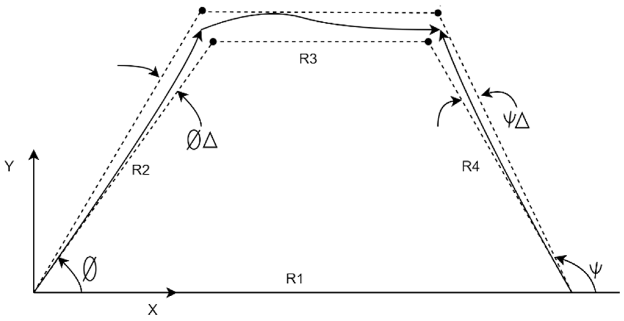
The flexible-link CM has fuzzy regions of and ψ as shown in Figure 4. The fuzzy region of and ψ can be represented by the TFN.
These regions specifically encompass variables and ψ , demonstrating a range of values rather than fixed points. This flexibility in values is essential for the dynamic operation of CMs, allowing for a more adaptive response under varying conditions. The fuzzy regions of changes in   ( ) and changes in ψ   ( ψ ) are effectively captured using TFNs, a method well suited for representing uncertainty and gradation within specific boundaries.
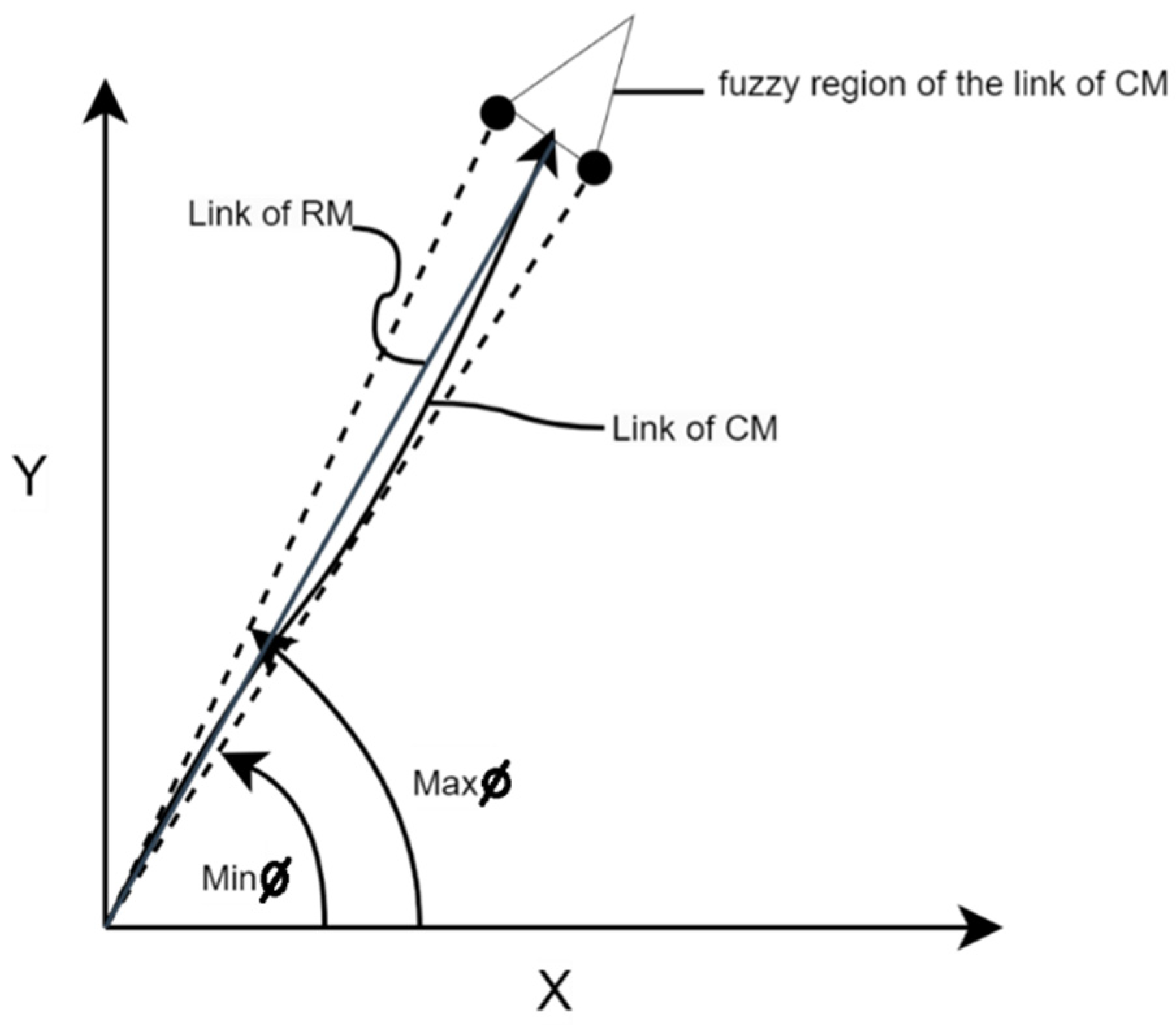
Figure 5 further clarifies these concepts by marking the maximum and minimum values of that define the boundaries of the fuzzy region associated with this variable. These boundaries are crucial, as they delineate the extent of variation allowed for , ensuring that the operational parameters remain within a controllable range. Within this framework, the rigid-mechanism (RM) link operates under a different assumption, in which the average value of is taken as the core of the TFN. This average serves as a central reference point around which fuzzy logic operations are structured, simplifying the complexity inherent in handling completely flexible systems.
The synthesis of these fuzzy regions extends beyond a single variable, addressing multiple regions involving and ψ within the CMs. These regions are precisely represented by TFNs, which highlight the complex, multilayered control required for function generation across various regions. TFNs offer a structured yet adaptable framework for interpreting input data, which is crucial for managing multiregion function-generation tasks. This approach allows for a more sophisticated manipulation of input-to-output angles, tailored to meet diverse operational requirements while maintaining precision and adaptability in CMs.
To navigate through and utilize these fuzzy regions effectively, fuzzy functions were constructed specifically to pass through these regions. This passage is facilitated by the fuzzy lengths of the links in the CMs, which are variable parameters that can be tuned according to the specific requirements of the task. The adaptability provided by these fuzzy lengths is pivotal because it allows the mechanism to maintain functionality across a spectrum of different operating conditions, thereby enhancing the robustness and reliability of the system.
The intricate relationship between the flexible and the assumed rigid components of the CMs, as delineated by the fuzzy regions and their corresponding TFNs, forms the backbone of the fuzzy model strategy. This strategy is essential for achieving precise control over the system’s output through a continuous modulation of the input angles, underpinned by a mathematical model that accommodates uncertainty and variability. The use of fuzzy logic not only enriches the control mechanism’s capability to handle diverse scenarios but also underlines the importance of a well-thought-out design and configuration in modern control systems.

3.3. The Fuzzy Freudenstein’s Equation

The three-point function synthesis of a four-bar linkage refers to the design process that aims to ensure the linkage achieves three specific positions. Freudenstein’s equation is used for the synthesis process. Exploring this slightly more deeply, the Freudenstein equation is a method for transforming the geometric problem of four-bar linkage synthesis into an algebraic problem that can be solved readily. It converts the three specified positions of the input and output cranks into a single polynomial equation.
The Freudenstein’s equation for three-point function synthesis is formulated as follows:
K 1 cos 1 + K 2 cos ψ 1 + K 3 = cos 1 ψ 1 K 1 cos 2 + K 2 cos ψ 2 + K 3 = cos 2 ψ 2 K 1 c o s 3 + K 2 c o s ψ 3 + K 3 = c o s 3 ψ 3
where angles of the input link 1 ,   2 ,   a n d   3 and angles of the output link ψ 1 ,   ψ 2 ,   a n d   ψ 3 .
Equation (4) allows us to calculate the lengths of the four bars that constitute the mechanism given the three desired output positions. By solving this equation, exact dimensions for the linkages to achieve the desired motion are obtained. The resulting mechanisms can be then tested to ensure they provide the desired output.
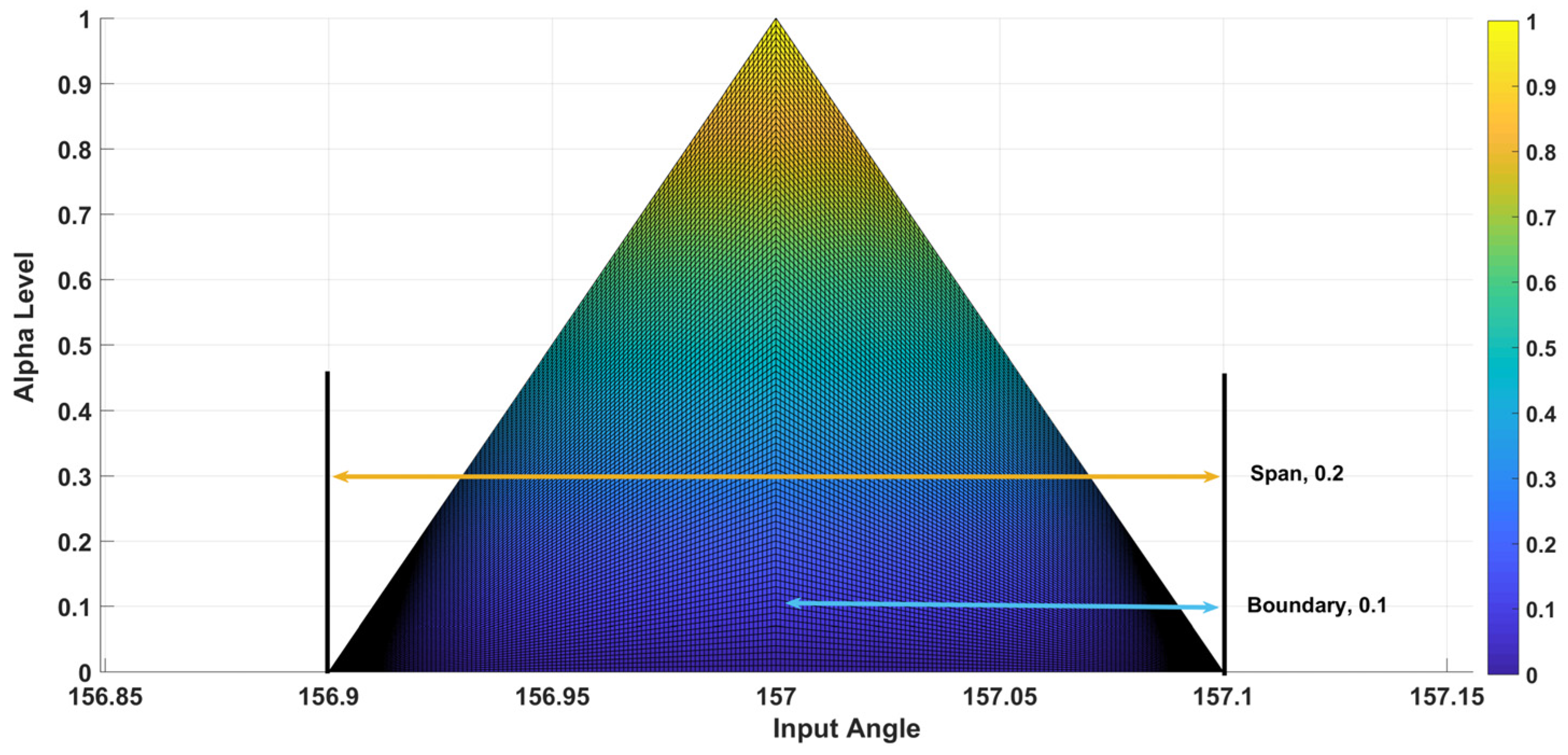
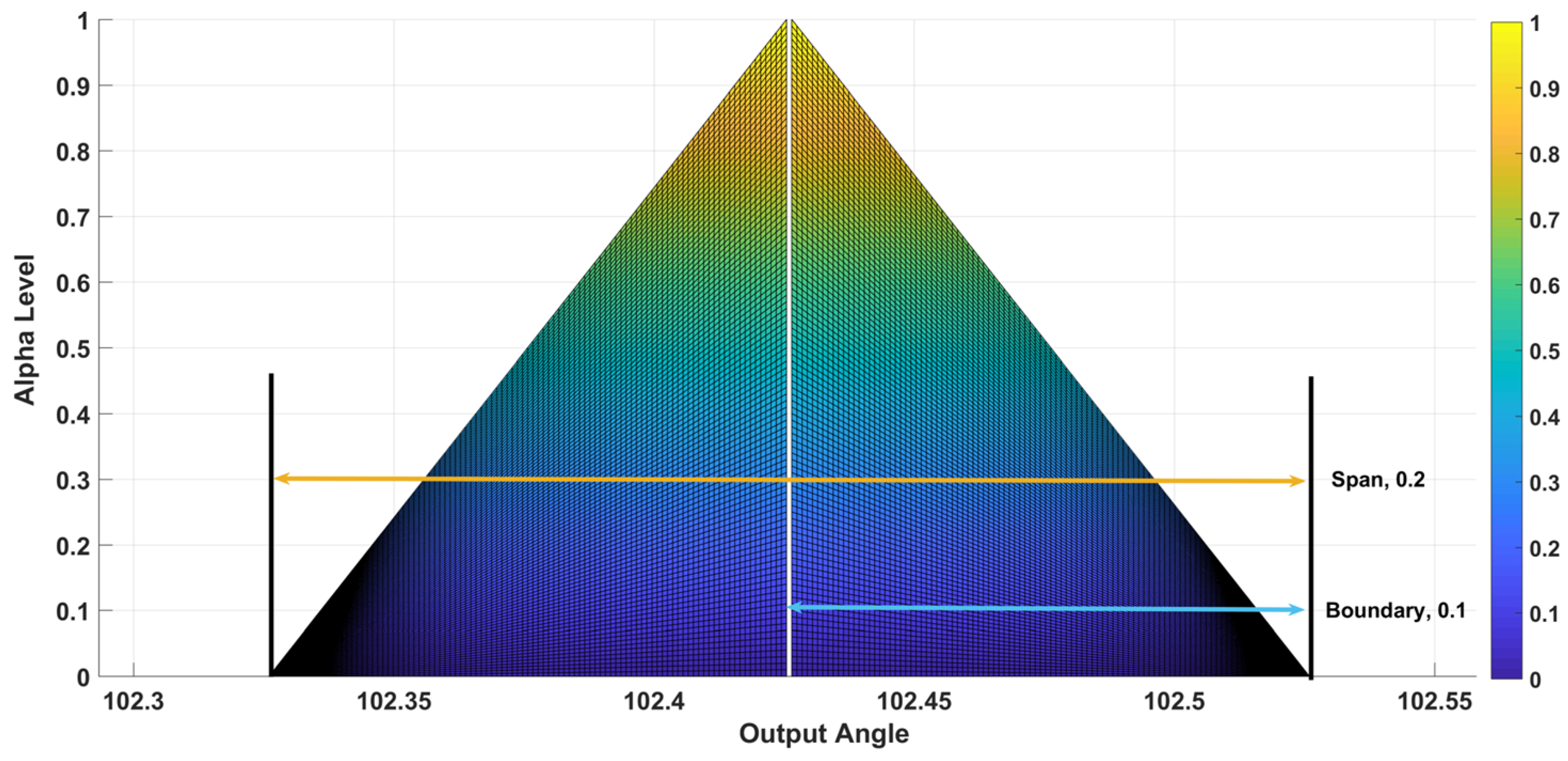
The compliant mechanism is dimensionally synthesized using three fuzzy input angles and their corresponding fuzzy output angles, which are based on the alpha level of the TFN in (3). These regions are shown as fuzzy numbers with boundaries and cores in Figure 6 and Figure 7, instead of crisp numbers. The boundaries of the input and output TFNs encompass the complete range of input and output angles for which the membership function values lie between zero and one. Conversely, the span of these angles includes all values where the membership function exceeds zero. Specifically, the span of a TFN corresponds to the zero-alpha-level interval number. The boundaries at these zero-alpha levels represent the differences in the lengths of CMs compared to rigid mechanisms. This variation is quantified by averaging these differences at the unity alpha level, as illustrated in the figures provided.
The synthesis function generation of CMs relies on the fuzzy regions that are formed by these input–output angles. The fuzzy regions reflect the variability of the CMs’ links, as shown in Figure 8.
When the links are not precise, there are countless output functions, and each output function results from a mix of the three links at different degrees, so that Freudenstein’s equation for a group of fuzzy links is
K 1 α cos i α ± K 2 α cos ψ i α + K 3 α = cos i α ψ i α
w h e r e   K i α = K i : K i α α ,   i α = i : i α α ,   ψ i α = ψ i : ψ i α α , K i α , ψ i α , i α T F N ,   α 0 , 1 ,   i = 1 , 2 , 3

4. Parametric Form and Newton’s Method

4.1. Parametric Form

The parametric form of a fuzzy number provides a way of expressing a fuzzy number in terms of three parameters: the core value, and the lower and upper bounds of the uncertainty or fuzziness. The most used parametric form is the TFN, which Zadeh in [27] introduced to provide a more intuitive way of representing fuzzy numbers. One way to write the TFN is to use one parameter ( α ) between 0 and 1 to show the three parameters, as in (3) and Figure 2. Zadeh [3] produced the idea of fuzzy numbers and used the TFN as a special example. This way makes it easier to perform addition and scalar multiplication on fuzzy numbers by the extension principle [4]. The following shows the parametric form of the nonlinear Freudenstein’s equation for fuzzy links:
K _ 1 α cos _ i α + K _ 2 α cos ψ _ i α + K _ 3 α = cos _ i α ψ _ i α   K ¯ 1 α cos ¯ i α + K ¯ 2 α cos ψ ¯ i α + K ¯ 3 α = cos ¯ i α ψ ¯ i α
where K _ i ,   _ i , and ψ _ i are the minimum limits of the TFNs at the zero-alpha level and K ¯ i ,   ¯ i , and ψ ¯ i are the maximum limits of these TFNs at the same zero-alpha level.

4.2. Newton Method

As [3] states, the equation presupposes that a solution to the system of equations exists, and then applies the Newton’s method to find an approximate solution. Newton’s method requires starting with an initial guess and using the partial derivatives of the equation to compute the unknown quantities h ( α ) and k ( α ) , which are the adjustments to the initial guess. These adjustments are then used to obtain a new approximation x 1 , and the process is repeated until the approximate solution converges to the true solution.
The problem shows a recursive procedure for obtaining the approximation, which involves modifying the guess with the adjustments. The rate of convergence of Newton’s method can be related to the maximum value of the corrections h n ( α ) and k n ( α ) via a lemma called Kantorovich’s lemma. This lemma states that if the Jacobian matrix of the system of equations is Lipschitz continuous with a constant L, then the maximum value of the corrections at step n, h n ( α ) and k n ( α ) , satisfy the inequality:
m a x h n α ,   k n α L 2     m a x h n 1 α ,   k n 1 α 2
In other words, the maximum value of the corrections at each iteration is at most half the square of the maximum value of the corrections at the previous iteration, multiplied by the Lipschitz constant L 2 . This implies that the rate of convergence of the Newton’s method is quadratic, meaning that the number of correct digits doubles at each iteration.
If Newton’s method converges to the true solution, then the maximum value of the corrections must go to zero as n goes to infinity. This is because if the solution is reached, then F _ ( x _ n ,   x ¯ n , α ) = c _ ( α ) and F ¯ ( x _ n ,   x ¯ n ,   α ) = c ¯ ( α ) , which implies that h n α = 0 and k n α = 0 . Therefore, in the limit as n goes to infinity, the maximum value of the corrections goes to zero as well, and the approximated solution converges to the true solution.
The rate of convergence of the Newton’s method is related to the Jacobian matrix and the Lipschitz constant c in the sense that the closer the Jacobian matrix is to the true value, and the larger the Lipschitz constant c, the faster the algorithm will converge to the solution.
The Jacobian matrix tells us how fast the function changes at a given point. In addition, Jacobian matrix approximates the function locally and determines the direction and distance to move towards the solution. If the derivative of the Jacobian matrix is more accurate and closer to the true value, the updated guess will be closer to the solution, and the convergence will be faster.
The Lipschitz constant c, on the other hand, is a measure of how “smooth” or well behaved the function is. A function that is Lipschitz continuous with a higher c value means that the rate of change of the function is bounded by a constant. This makes it easier to predict how the function will behave locally, and therefore makes the algorithm more stable and less prone to overshooting or oscillating around the solution.

4.3. Fuzzy Lengths for CMs

The parametric form of Freudenstein’s equation in (6) gives the Ks, which are used to estimate the CMs’ lengths as follows:
K 1 = R 1 R 4 ,       K 2 = R 1 R 2 ,       K 3 = R 1 2 + R 2 2 + R 4 2 R 3 2 2 R 2 R 4
where R 1 is the length of ground link, R 2 is the length of the crank link, R 3 is the length of the coupler link, and R 4 is the length of the follower link.
Parametric fuzzy arithmetic is applied to estimate the fuzzy lengths of the links, which are obtained by solving the equations in (8) with the assumption that the length of the ground link is one.
Consider two parametric fuzzy numbers, Q ~ 1 and Q ~ 2 , which can be expressed as
Q ~ 1 = Q 1 _ ( α ) ,   Q 1 ¯ ( α ) ,     Q ~ 1 = Q 2 _ ( α ) ,   Q 2 ¯ ( α )
where α is a value between 0 and 1. Beside the arithmetic operations of the extension principle that was mentioned above, all standard parametric fuzzy arithmetic operations can be defined using the following formula:
Q ~ 1 Q ~ 2 = Q 1 Q 2 Q 1 Q 1 α , Q 2 Q 2 α ,       α [ 0 , 1 ] }
Here, “ ” represents any binary operation such as addition, subtraction, multiplication, division, or power. The binary operation can be expressed as
Q ~ 1 + Q ~ 2 = Q 1 _ α + Q 2 _ α , Q 1 ¯ α + Q 2 ¯ α
Q ~ 1 Q ~ 2 = Q 1 _ α Q 2 ¯ α , Q 1 ¯ α Q 2 _ α
k · Q ~ 1 = k · Q 1 _ α , k · Q 1 ¯ α ,   k > 0 k · Q 1 ¯ α , k · Q 1 _ α ,   k < 0     k R
Q ~ 1 · Q ~ 2 = min Q 1 _ α · Q 2 _ α ,   Q 1 _ α · Q 2 ¯ α , Q 1 ¯ α · Q 2 _ α , Q 1 ¯ α · Q 2 ¯ α , max Q 1 _ α · Q 2 _ α ,   Q 1 _ α · Q 2 ¯ α , Q 1 ¯ α · Q 2 _ α , Q 1 ¯ α · Q 2 ¯ α  
1 Q ~ 1 = 1 Q 1 ¯ α , 1 Q 1 _ α ,   0 Q ~ 1 , ,   0 Q ~ 1
Q ~ 1 Q ~ 2 = Q ~ 1 · 1 Q ~ 2 = Q 1 _ α ,   Q 1 ¯ α · 1 Q 2 ¯ α , 1 Q 2 _ α ,   0 Q ~ 1 , ,   0 Q ~ 1
Finally, the parametric form of fuzzy power can be expressed as
Q ~ 1 m = Q 1 _ α m ,   Q 1 ¯ α m ,       i f   m > 0   a n d   m   i s   o d d
If m > 0 and m is an even integer, the parametric form of fuzzy power will be
Q ~ 1 m = Q 1 _ α m ,   Q 1 ¯ α m , Q ~ 1 > 0 Q 1 ¯ α m ,   Q 1 _ α m , Q ~ 1 < 0 0 , max Q 1 _ α m ,   Q 1 ¯ α m , 0 Q ~ 1
By combining the Newton method and standard parametric fuzzy arithmetic operations, the fuzzy lengths of the CMs are obtained, as shown in the numerical examples in the following section.

4.4. Fuzzy Optimization

Fuzzy inference systems (FISs) are widely utilized in engineering and control systems to manage uncertainty and variability in decision-making processes. In the design and optimization of CMs, where traditional deterministic approaches struggle with nonlinear behavior and complexity, fuzzy optimization offers a more robust and adaptive solution.
By representing input and output parameters as TFNs, fuzzy optimization accounts for variability and imprecision in the design process. The Mamdani-type inference system is employed to assess multiple error metrics, which are classified into linguistic categories such as “less”, “medium”, and “more”. These metrics are processed through a set of fuzzy rules that evaluate the spread of errors and generate an optimized estimate for error correction.
The core of the optimization process involves a fuzzy inference system that evaluates deviations between crisp and fuzzy values at various points in the mechanism’s performance. The system applies membership functions to these deviations, which are then aggregated through fuzzy rules to produce a comprehensive error assessment. This output provides critical guidance for design adjustments, ensuring the mechanism operates within desired performance thresholds, even under uncertain input conditions.
By integrating fuzzy logic into the optimization framework, the system becomes highly resilient to variations and uncertainties in input parameters. This adaptability leads to the creation of more reliable and efficient mechanisms, particularly suited to addressing the nonlinear dynamics characteristic of compliant mechanisms. Thus, fuzzy optimization significantly enhances the design process, ensuring both flexibility and robustness in mechanism performance.

4.4.1. Inputs

The fuzzy inference system consists of six input variables, each representing different types of errors. Each input is categorized into three linguistic membership functions, less, medium, and more, represented by triangular membership functions. They are simple and computationally efficient, providing clear boundaries between different error categories. The “less” membership function handles values near the lower limit of the input range, indicating minimal error. The “medium” membership function handles intermediate values, representing moderate error. The “more” membership function handles values near the upper limit of the range, indicating severe error.

4.4.2. Output

The system outputs a single error criterion, which represents the overall severity of the error conditions based on the inputs. The output is divided into three linguistic categories, lower, center, and upper, using triangular membership functions. These categories correspond to varying levels of output error severity, from minor to moderate to critical. The system’s output serves as a decision-making tool for determining the necessary corrective actions based on the evaluated errors.

4.4.3. Fuzzy Rules

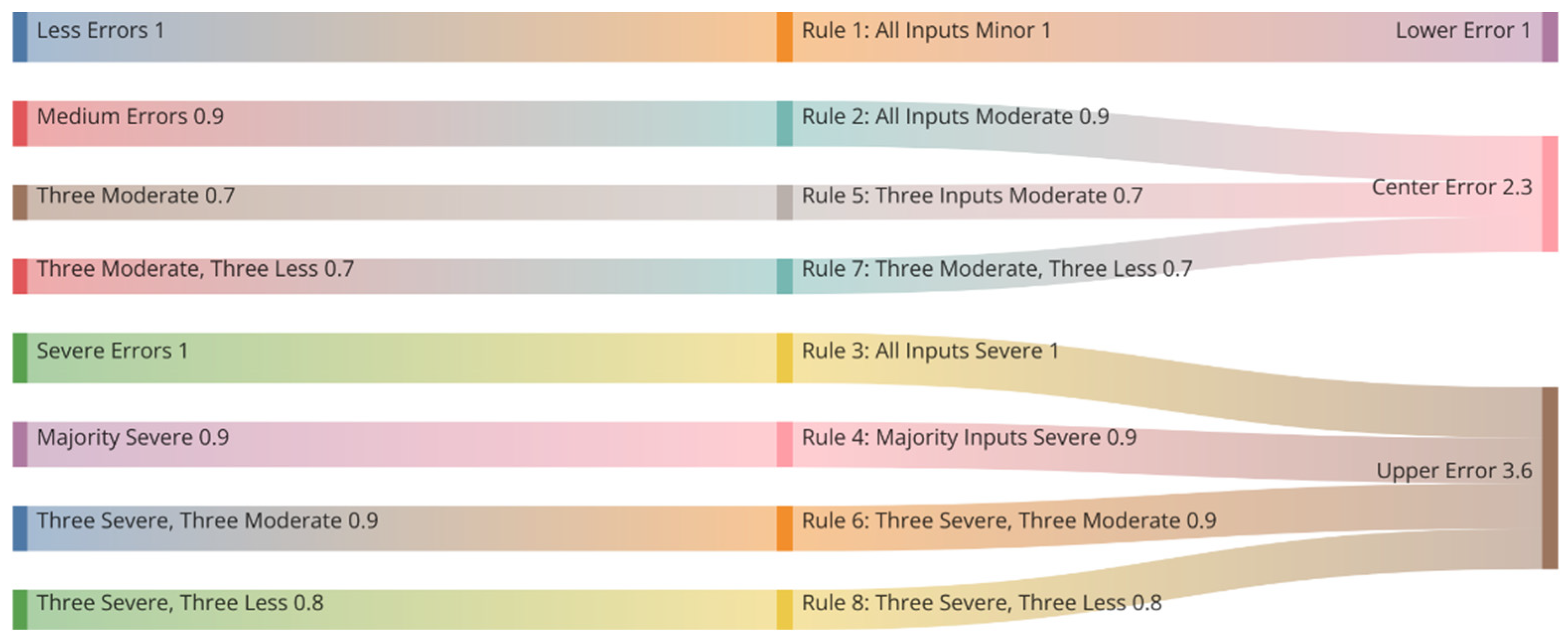
The fuzzy rules in this system are the core mechanism that defines how the inputs are processed to produce the output. The system uses eight rules to manage various combinations of input conditions. These rules follow the standard “if–then” format, using logical operators like “and” and “or” to handle different scenarios. To prioritize critical errors, weights are applied to the rules, ranging between 0.7 and 1. The weights ensure that critical conditions receive higher priority, while less critical conditions have reduced influence on the decision-making process. The Figure 9 below shows how the inputs are related to outputs through eight rules of the system.
The first rule covers situations where all input variables indicate minor errors. In such cases, the output is classified as lower, representing a minimal error criterion. This rule is assigned a full weight of 1, ensuring that when all inputs are classified as “less”, the system confidently outputs a low error criterion.
When all inputs indicate moderate error levels, the second rule comes into effect, classifying the output as center. This rule has a slightly reduced weight of 0.9, reflecting that while moderate errors are important, they are not as critical as situations involving severe errors. The weight ensures that moderate conditions are treated with less priority compared to more severe errors.
The third rule handles cases where all inputs signal severe errors. In such scenarios, the output is classified as upper, representing the highest error criterion. This rule is assigned the maximum weight of 1, indicating that the system treats these conditions with the highest priority and responds decisively.
For more complex situations where a majority of inputs (four or more) indicate severe errors, the fourth rule is triggered. This rule classifies the output as upper with a weight of 0.9, ensuring the system reflects the critical nature of having multiple severe errors, even if not all inputs are classified as “more”.
The fifth rule is designed to handle cases where any three or more inputs are classified as medium. The output is classified as center, with a reduced weight of 0.7, reflecting the moderate severity of these conditions. This ensures that while the system acknowledges the presence of moderate errors, it does not prioritize them as strongly as rules involving severe errors.
For intermediate cases where three inputs indicate severe errors and the other three inputs indicate moderate errors, the sixth rule applies. In such cases, the output is classified as upper, with a weight of 0.9. This reflects that the presence of multiple severe errors still dominates the decision, even when some inputs indicate less critical conditions.
When three inputs are classified as medium and the other three as less, the system triggers the seventh rule, classifying the output as center. The rule’s weight of 0.7 ensures that the system does not over-prioritize this scenario but still recognizes the moderate errors present.
Lastly, the eighth rule addresses cases where three inputs are classified as severe errors and the other three as minor errors. The output is classified as upper with a weight of 0.8. This ensures that severe errors have enough influence to result in a high error criterion but without overwhelming the decision-making process.

4.4.4. Defuzzification and Methods

The system uses the centroid method for defuzzification, calculating the center of gravity of the aggregated fuzzy sets to produce a crisp, numerical output. The rule aggregation uses the max method, ensuring that the highest membership value from the combined fuzzy sets influences the output. The min method is used for implication, allowing the system to handle conjunctions in a conservative manner, where the lowest membership value is selected for the rule condition.

5. Numerical Examples

To demonstrate the practical application of the methodologies discussed, a detailed numerical example is presented. This example illustrates the synthesis process of a compliant mechanism using the proposed parametric fuzzy approach, providing a clear understanding of how the theoretical concepts are implemented in practice.

5.1. Example 1

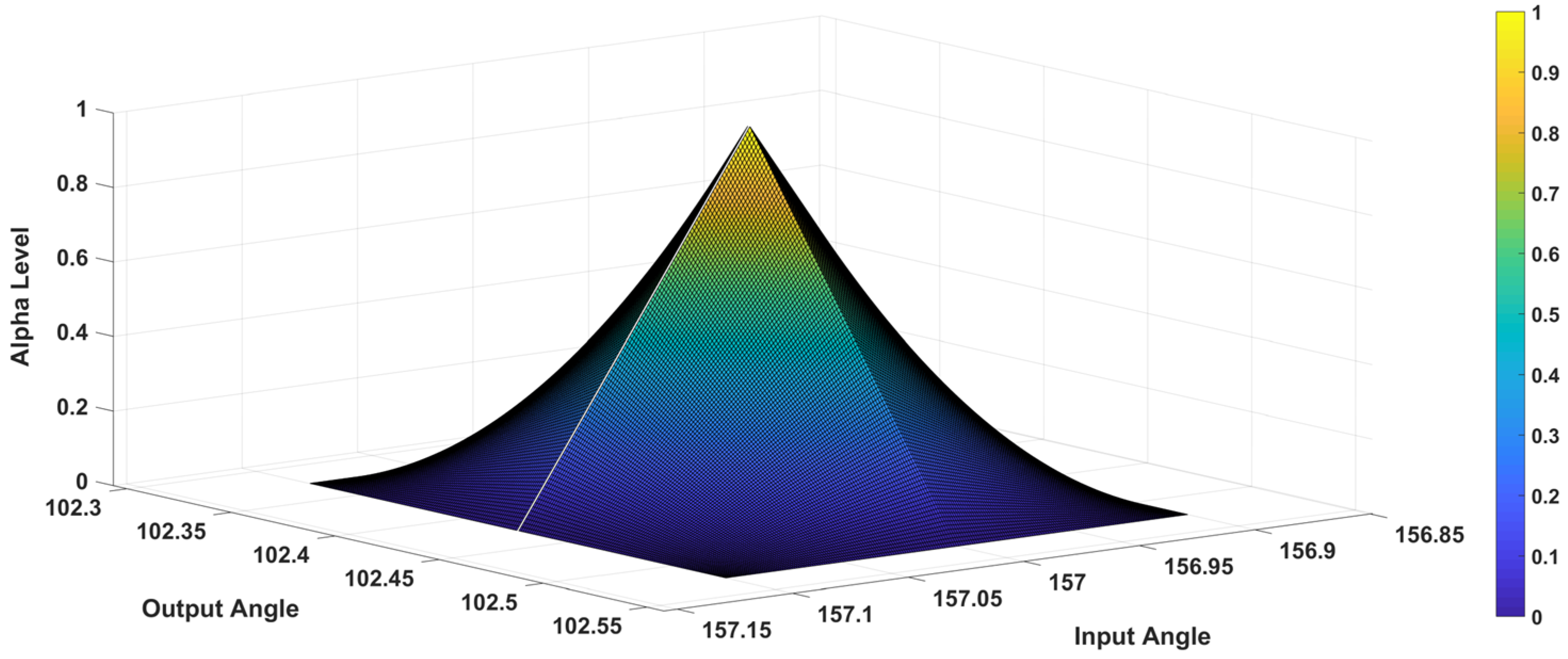
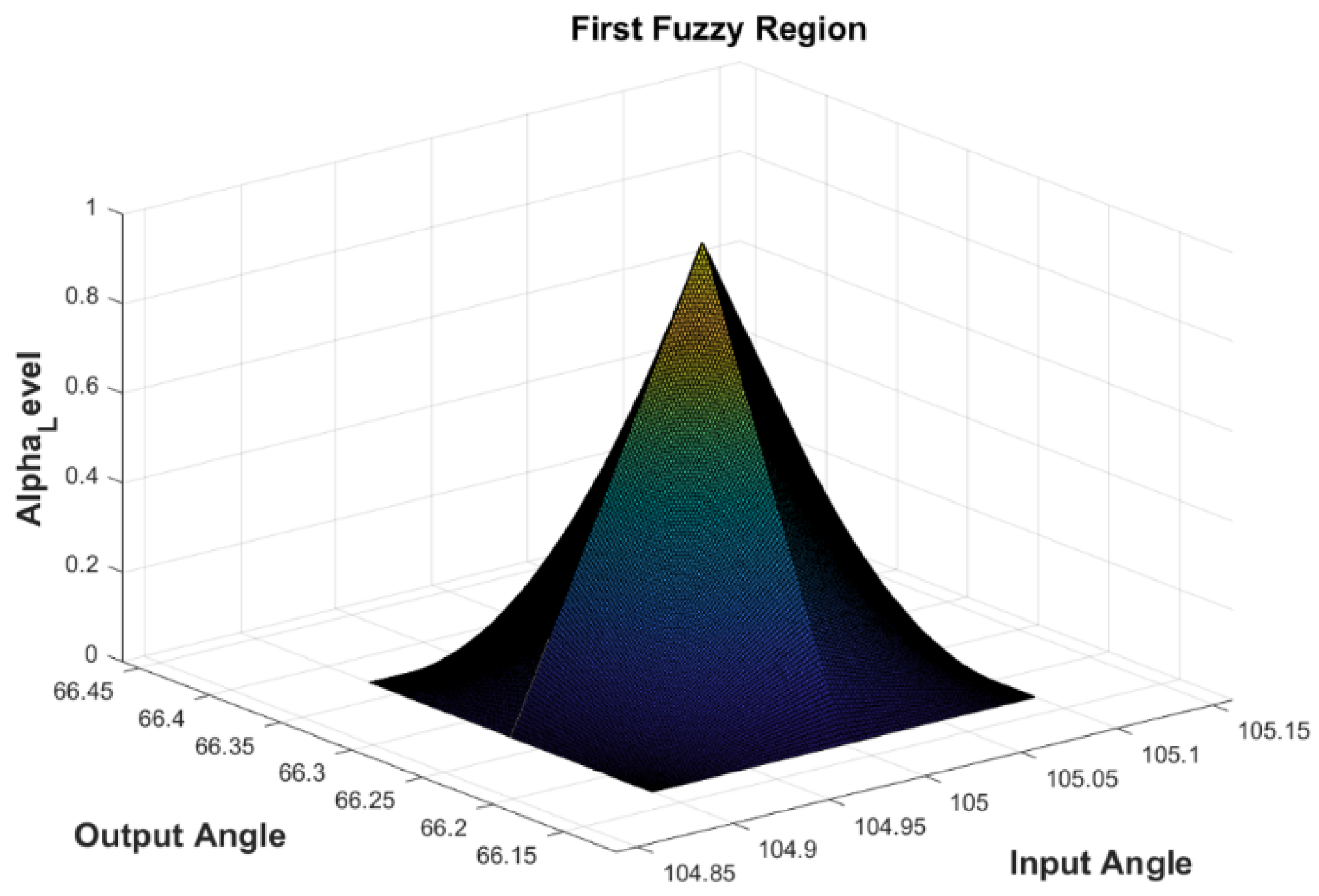
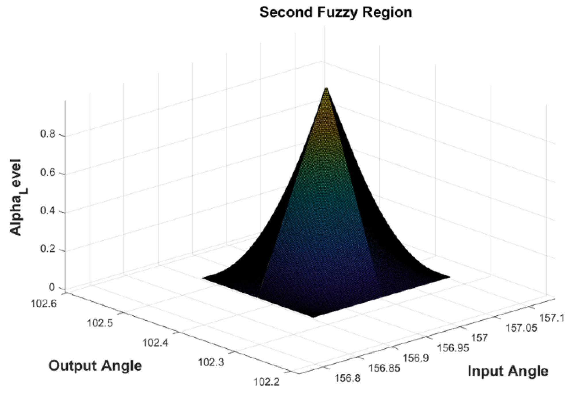
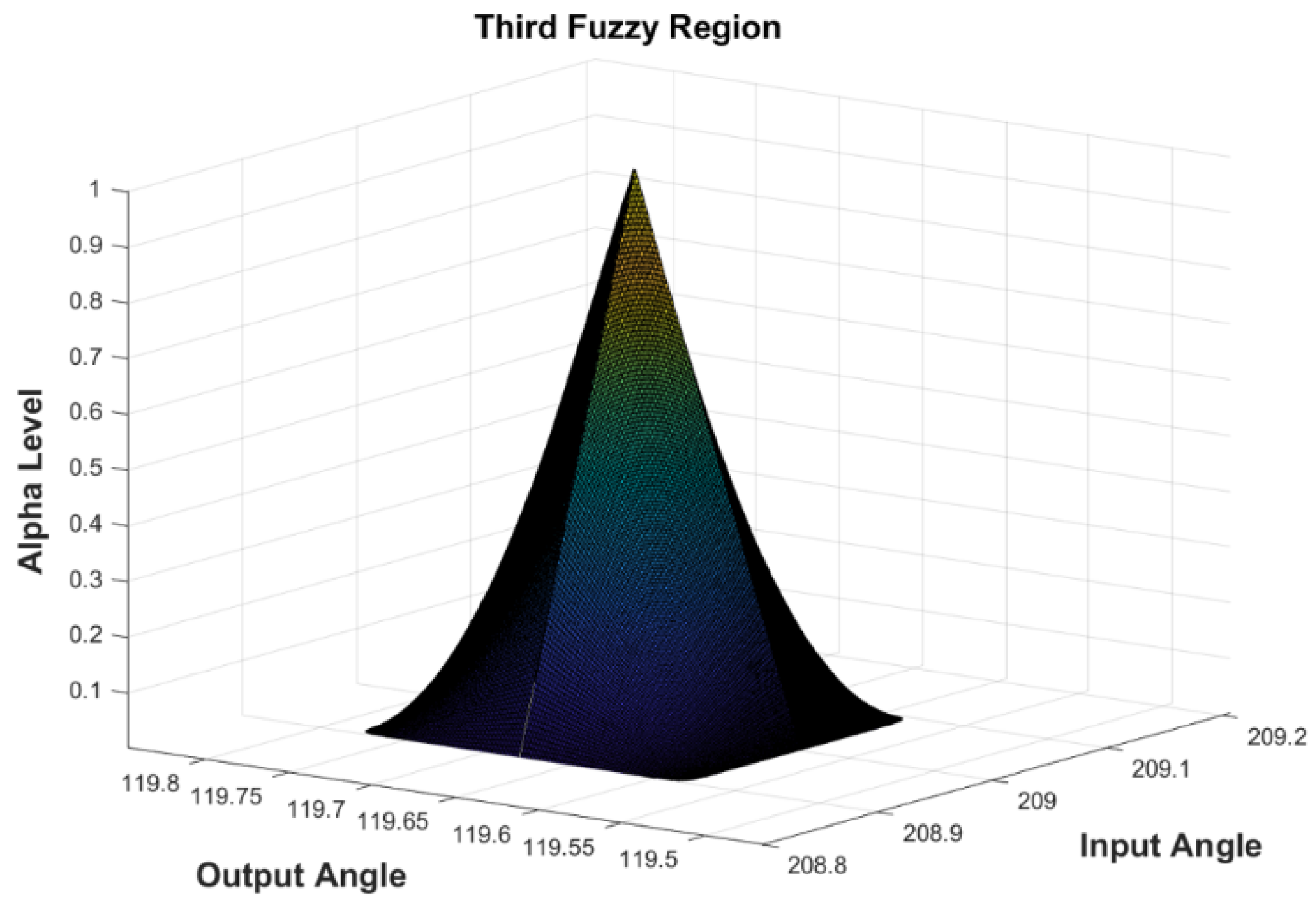
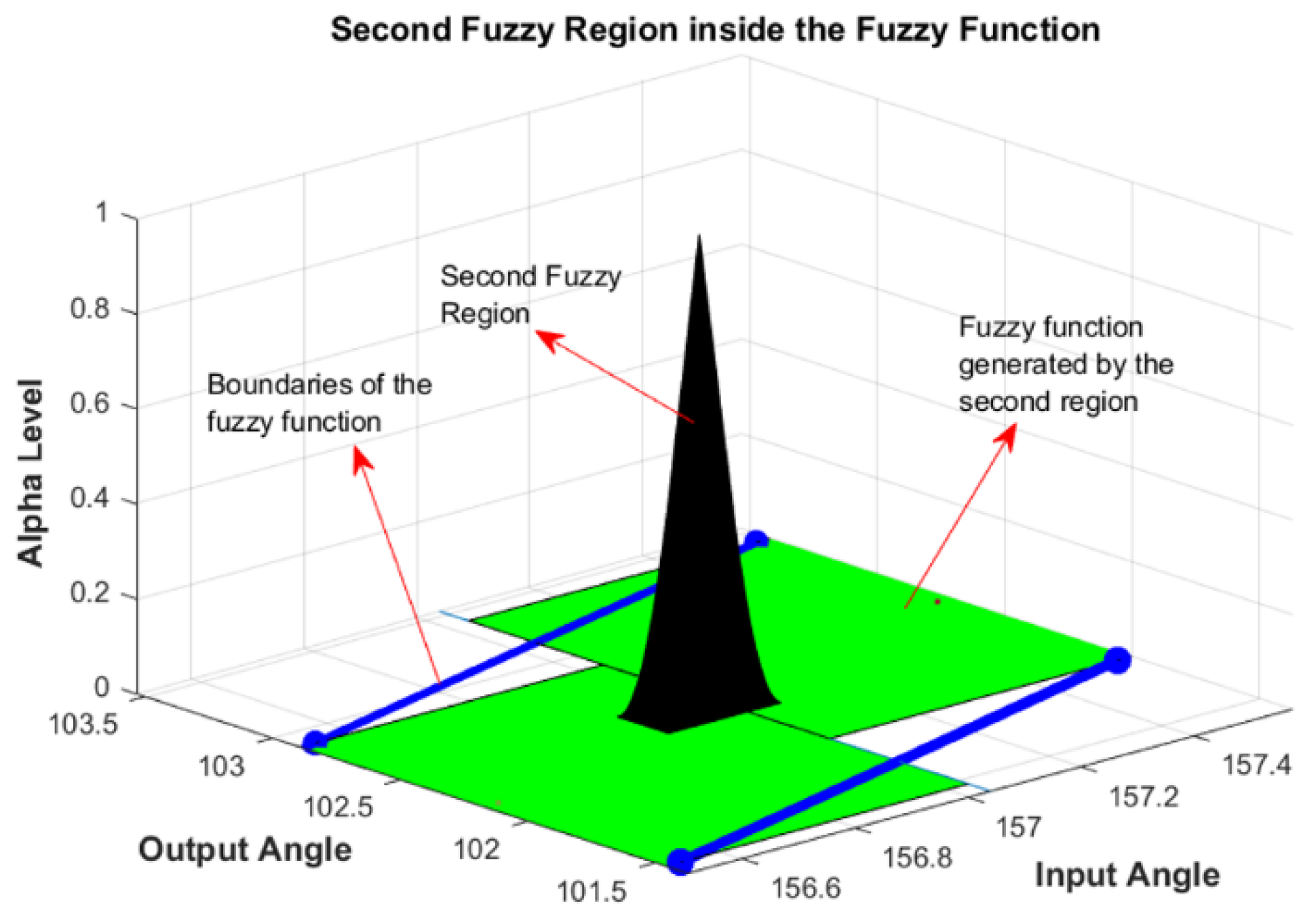
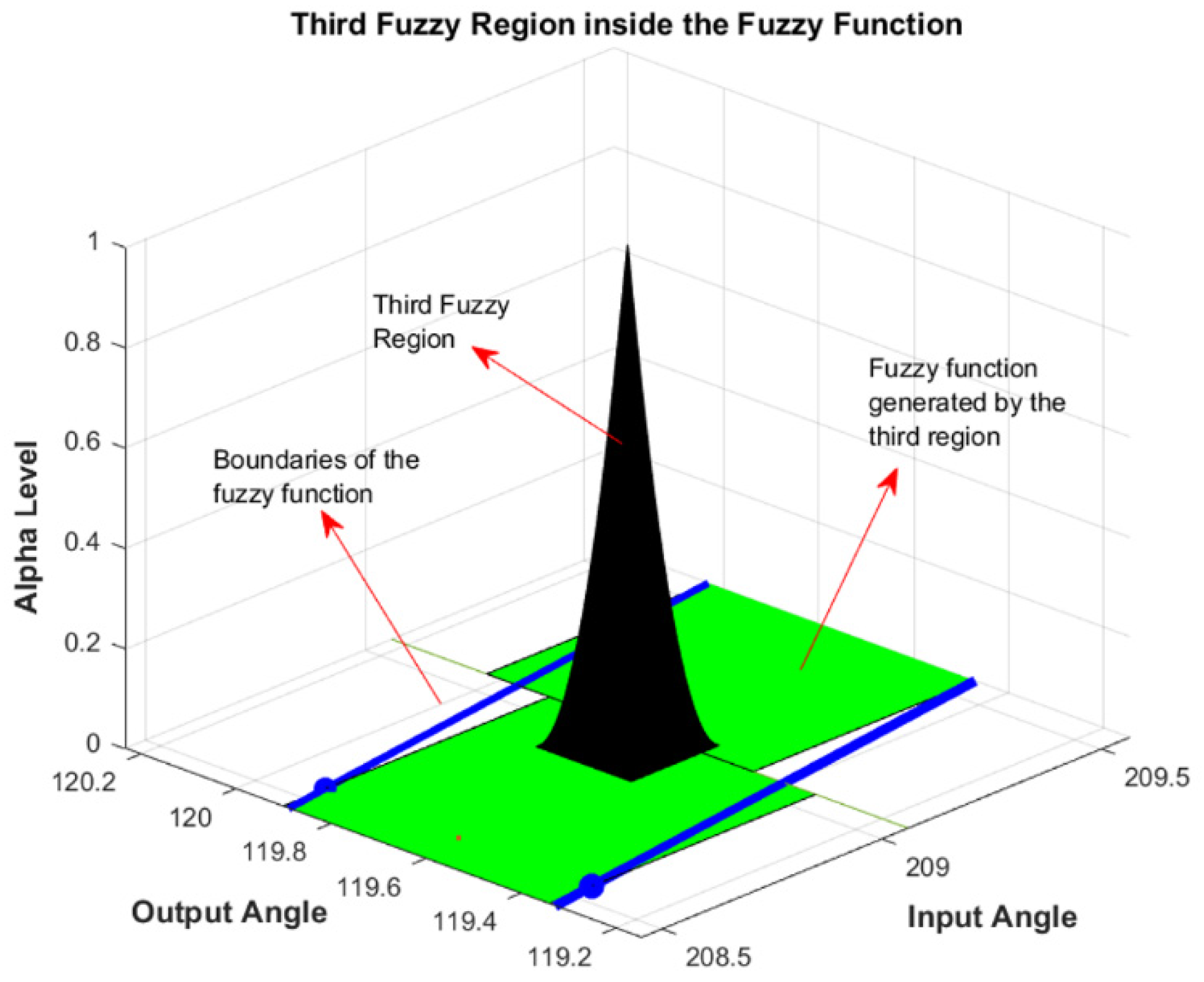
This example illustrates how to synthesize a compliant four-bar mechanism that can achieve certain output angles for a given set of input angles. The synthesis uses TFNs to account for uncertainties in the input and output parameters, which makes the design more resilient to variations in operating conditions. Suppose we have a CM whose input and output angles have uncertainties of = ψ = 0.2 ° ; then, the fuzzy region for synthesizing the CM is shown in Figure 10, Figure 11 and Figure 12 below. These fuzzy regions for the input angle ~ and the output angle ψ ~ cover the range of possible values for the angles, considering uncertainties.
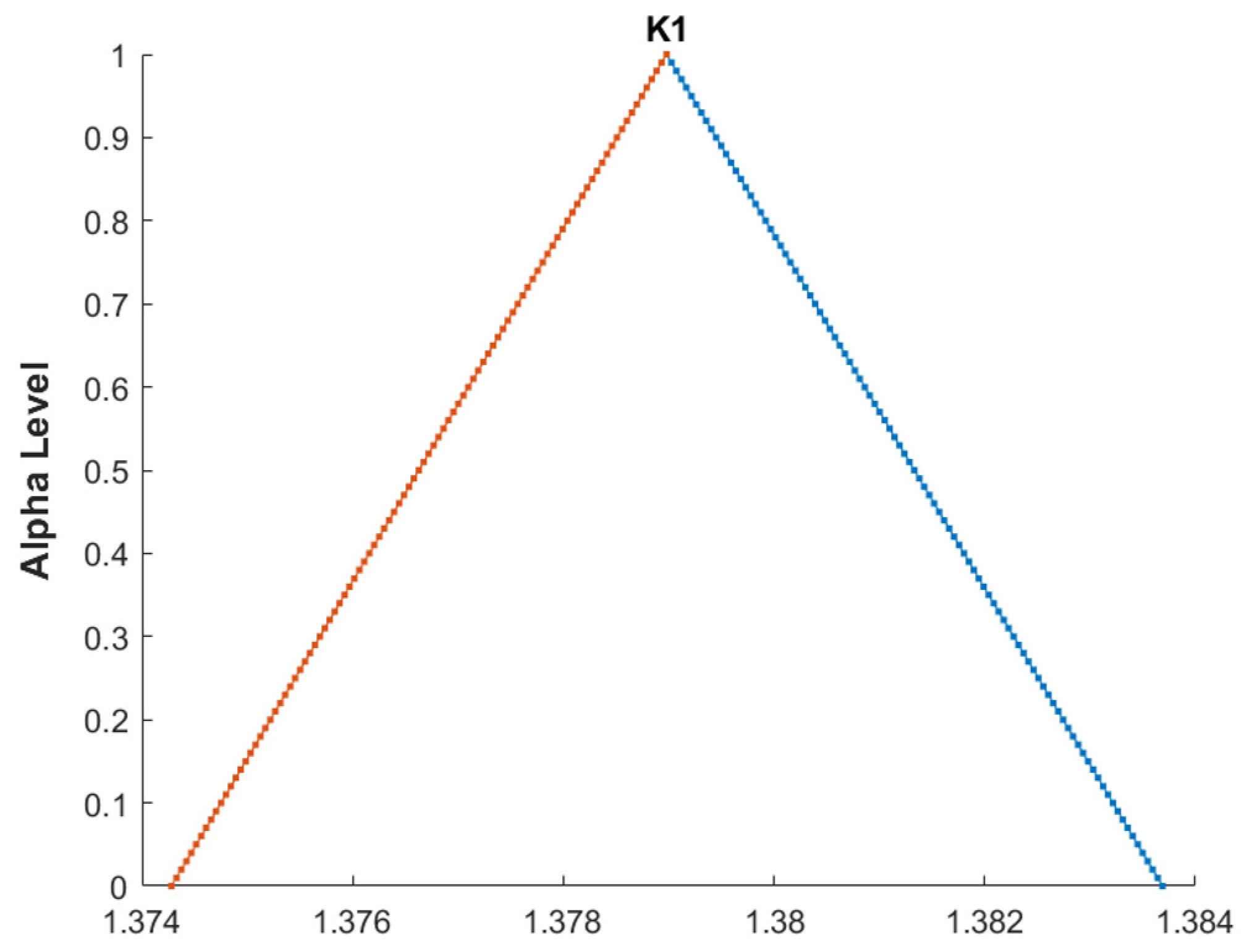
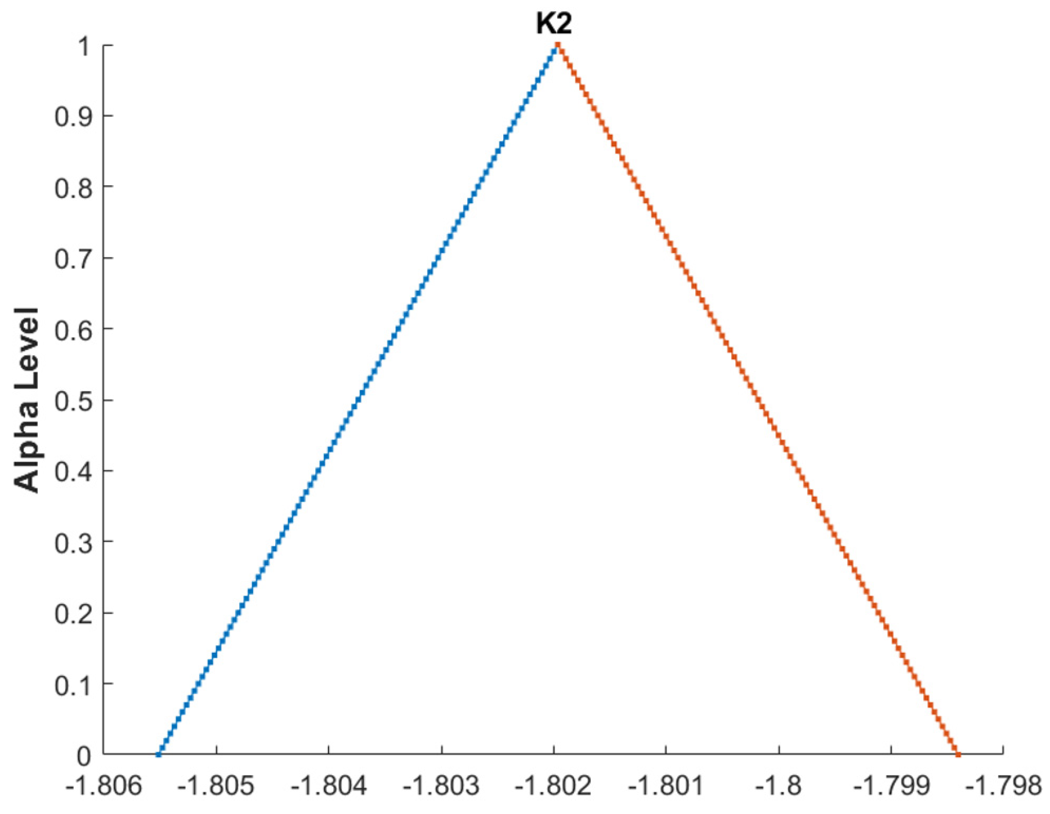
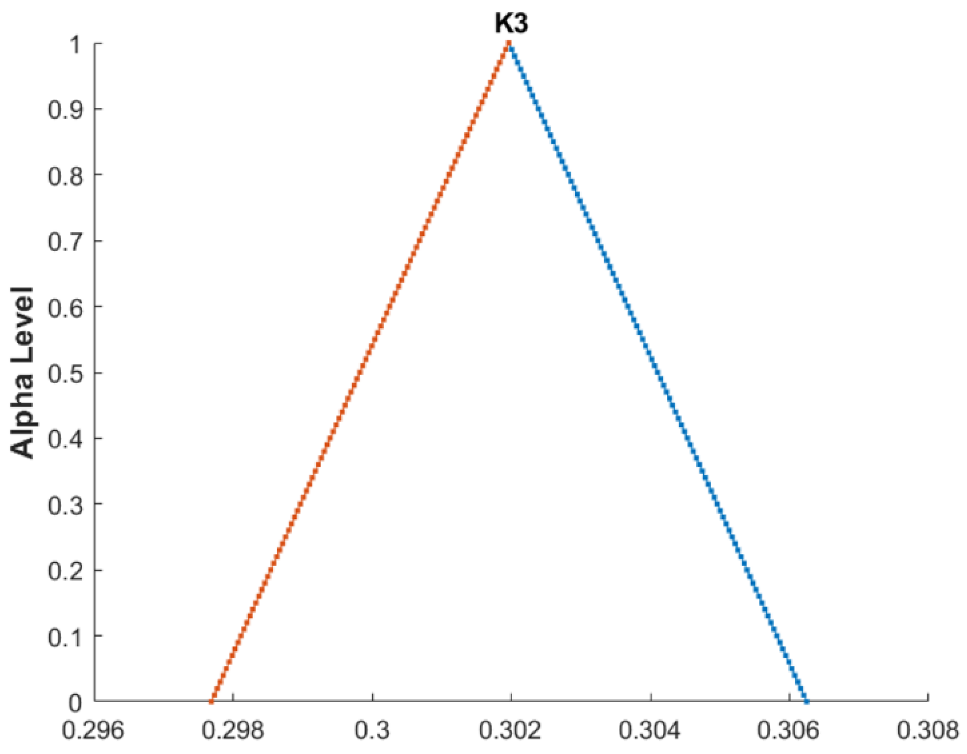
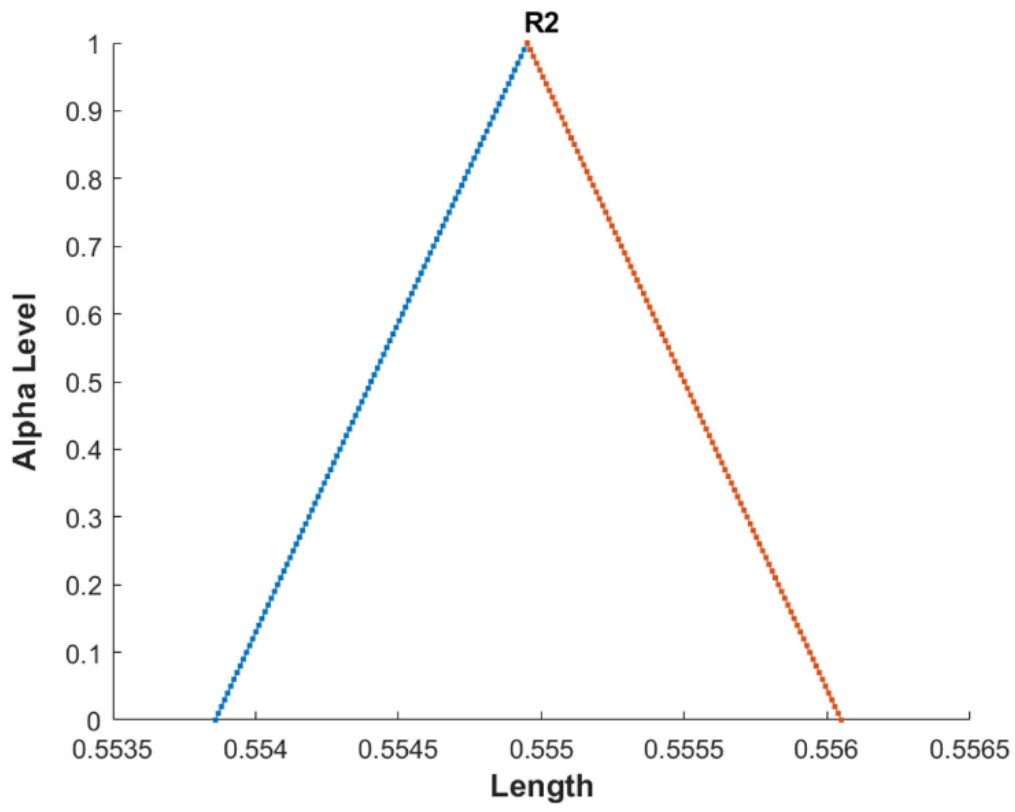
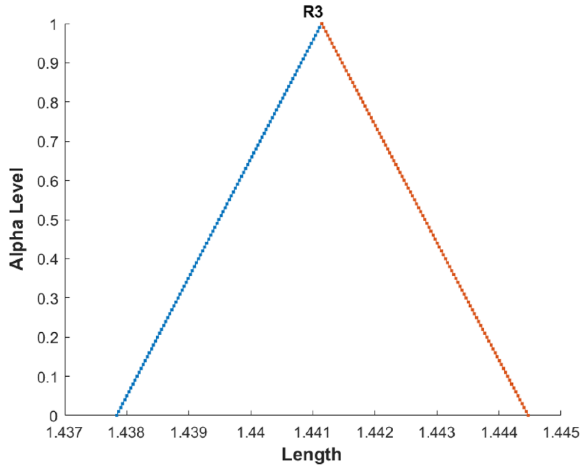
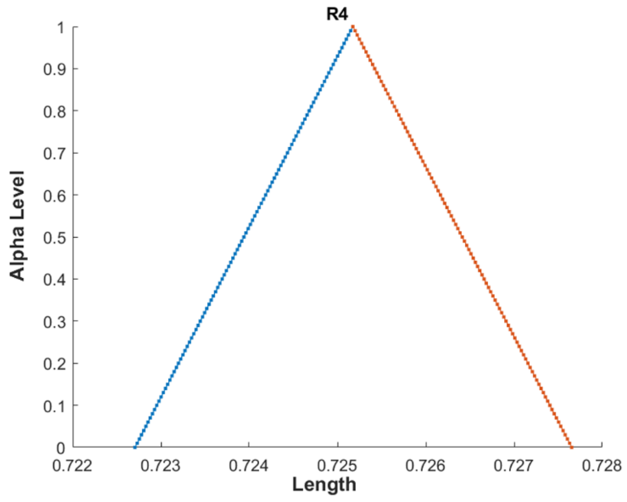
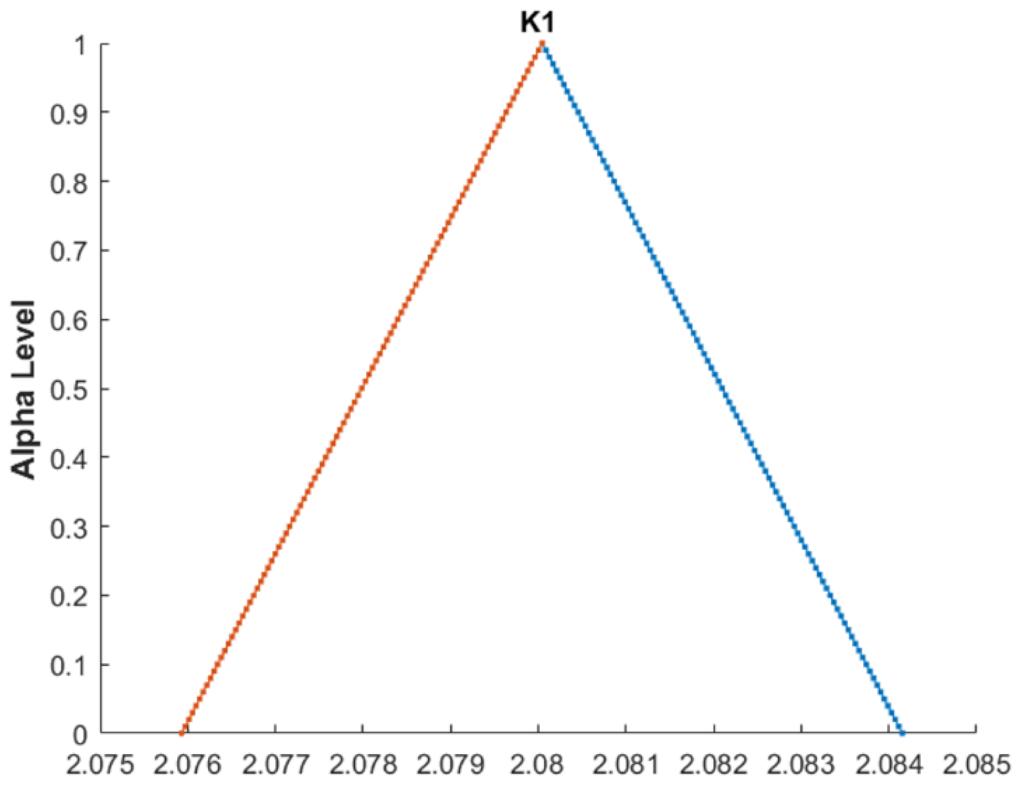
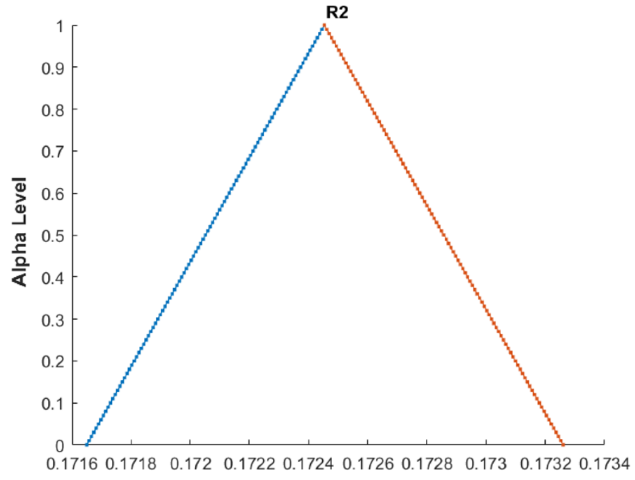
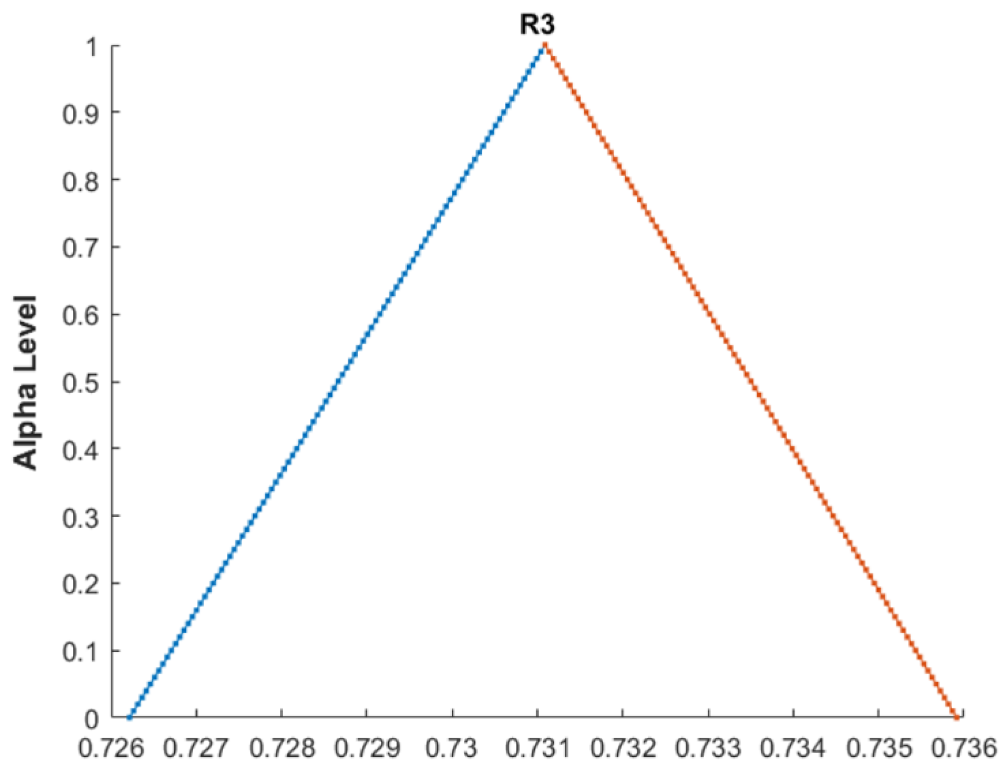
Freudenstein’s equation is applied to transform the geometric problem into an algebraic form, relating the input and output angles of the four-bar linkage and facilitating the synthesis process. The fuzzy input–output relationships are established using the parametric form of Freudenstein’s equation, with the zero-alpha level of the TFNs representing the boundaries of the fuzzy regions. The lengths of the crank (R2), coupler (R3), and rocker (R4) are determined as TFNs, which are crucial for achieving the desired input–output function. To visualize the fuzzy input and output angles, the constants K 1 , K 2 , and K 3 are introduced, which play a pivotal role in Freudenstein’s equation. These constants are essential in determining the link lengths R 2 , R 3 , and R 4 , represented as TFNs, as Figure 13, Figure 14, Figure 15, Figure 16, Figure 17 and Figure 18 illustrated.
Additionally, the fuzzy function of the compliant mechanism (CM) is introduced, representing the input–output relationship within the defined fuzzy regions. This function captures the variability in the system due to uncertainties in the input parameters, providing a comprehensive view of how the mechanism performs under different conditions. The resulting link lengths are displayed as fuzzy numbers, indicating the range of possible lengths that satisfy the input–output requirements.
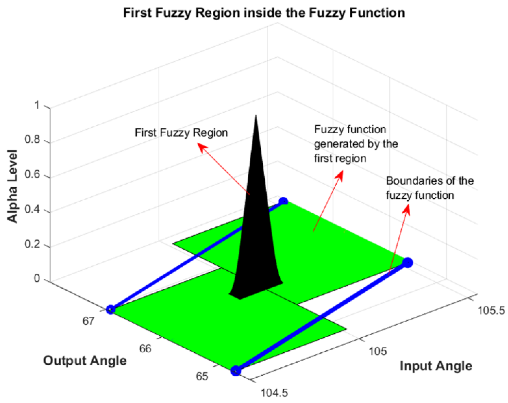
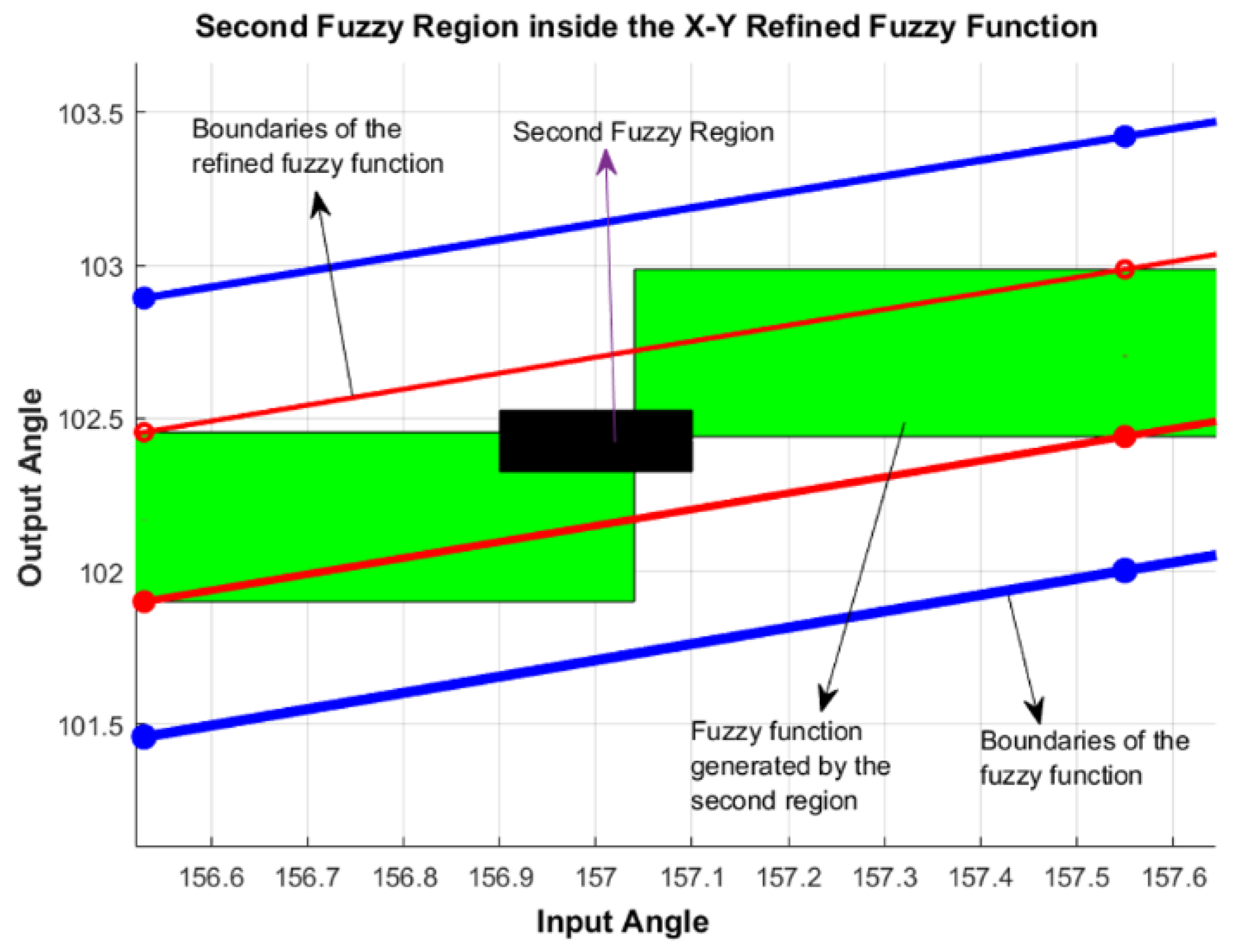
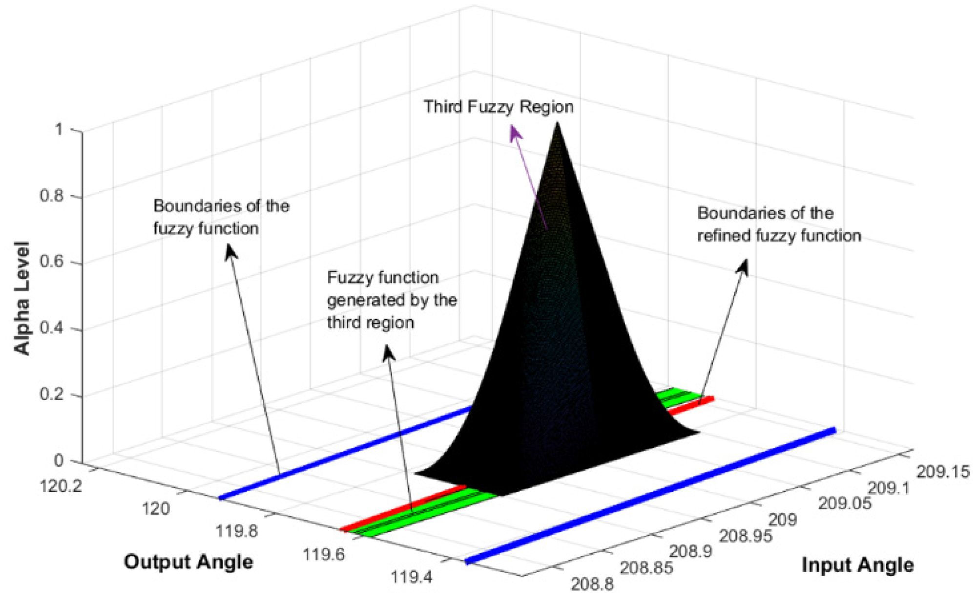
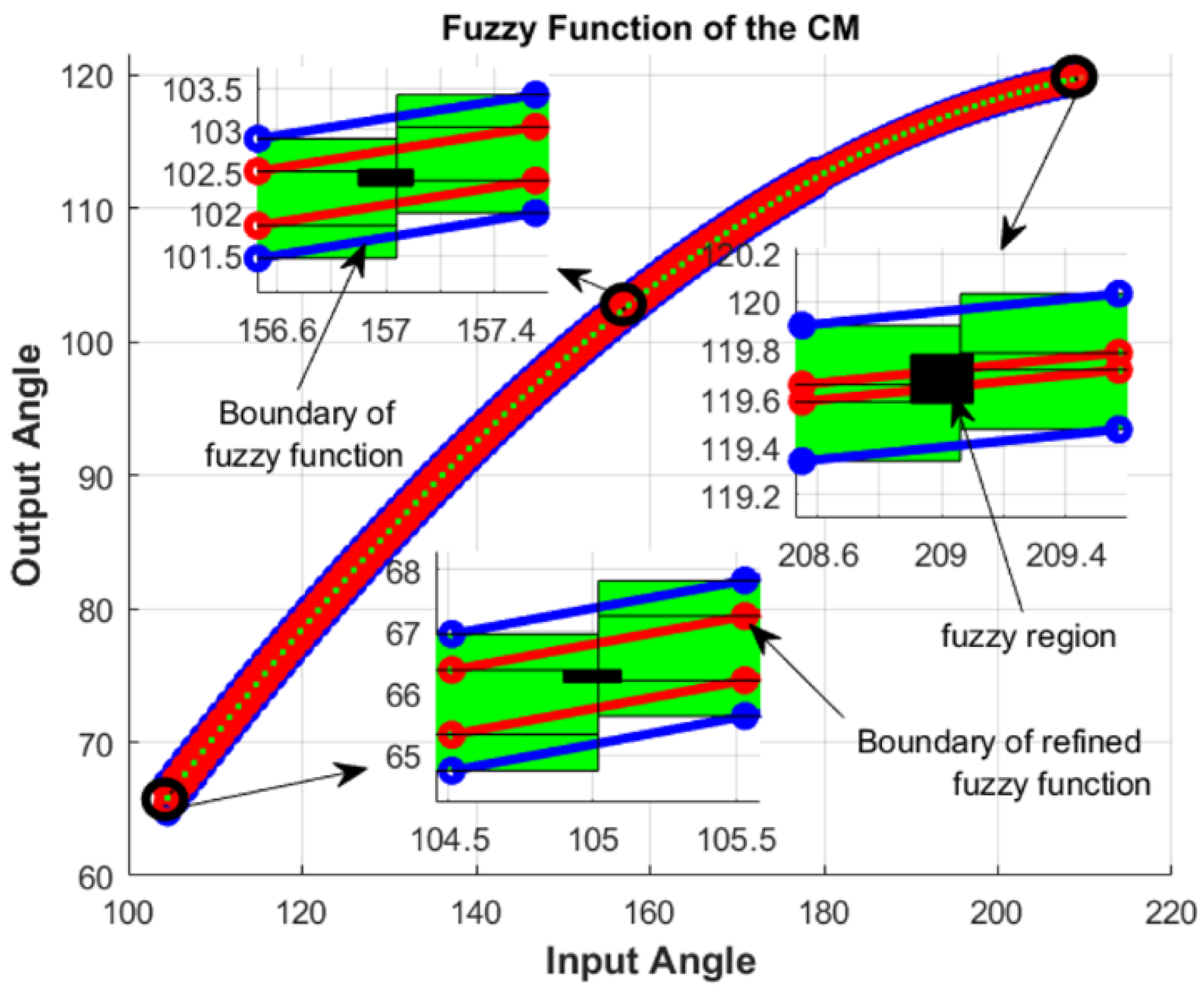
The fuzzy regions define the functional behavior of the CM as it traverses through them. These fuzzy functions are composed of rectangular boxes that illustrate the variation in the lengths of the CM links. The zero-alpha level of the fuzzy function is depicted by green boxes, which are bounded by the smallest and largest values of these fuzzy numbers. The three-dimensional membership functions of these fuzzy regions, formed by the fuzzy numbers of the CM links, are shown in Figure 19, Figure 20 and Figure 21. The three-dimensional membership functions depicted represent the uncertainties associated with the lengths of the compliant mechanism (CM)’s links. These functions encompass all possible values of the link lengths, as illustrated above in Figure 10, Figure 11 and Figure 12.
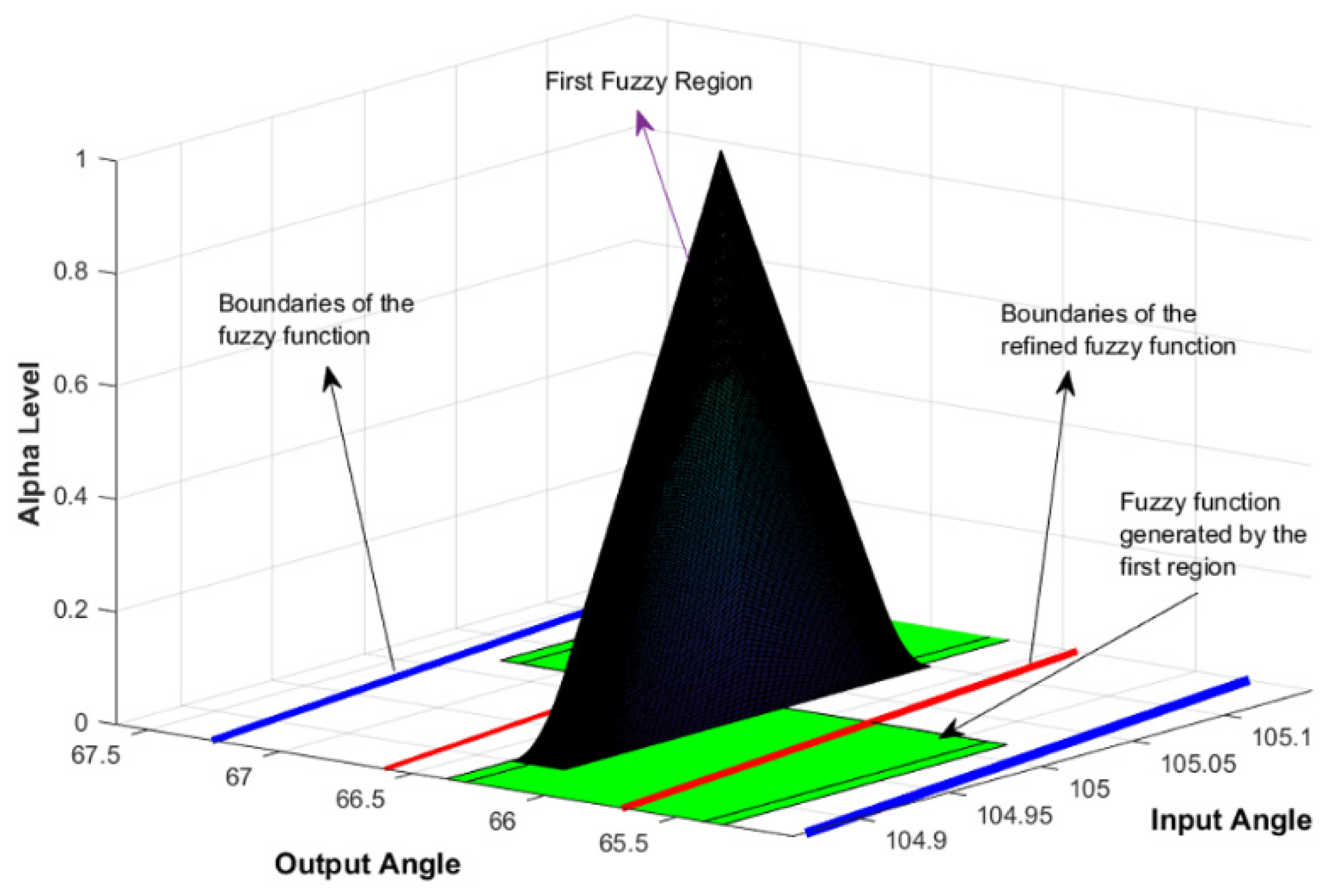
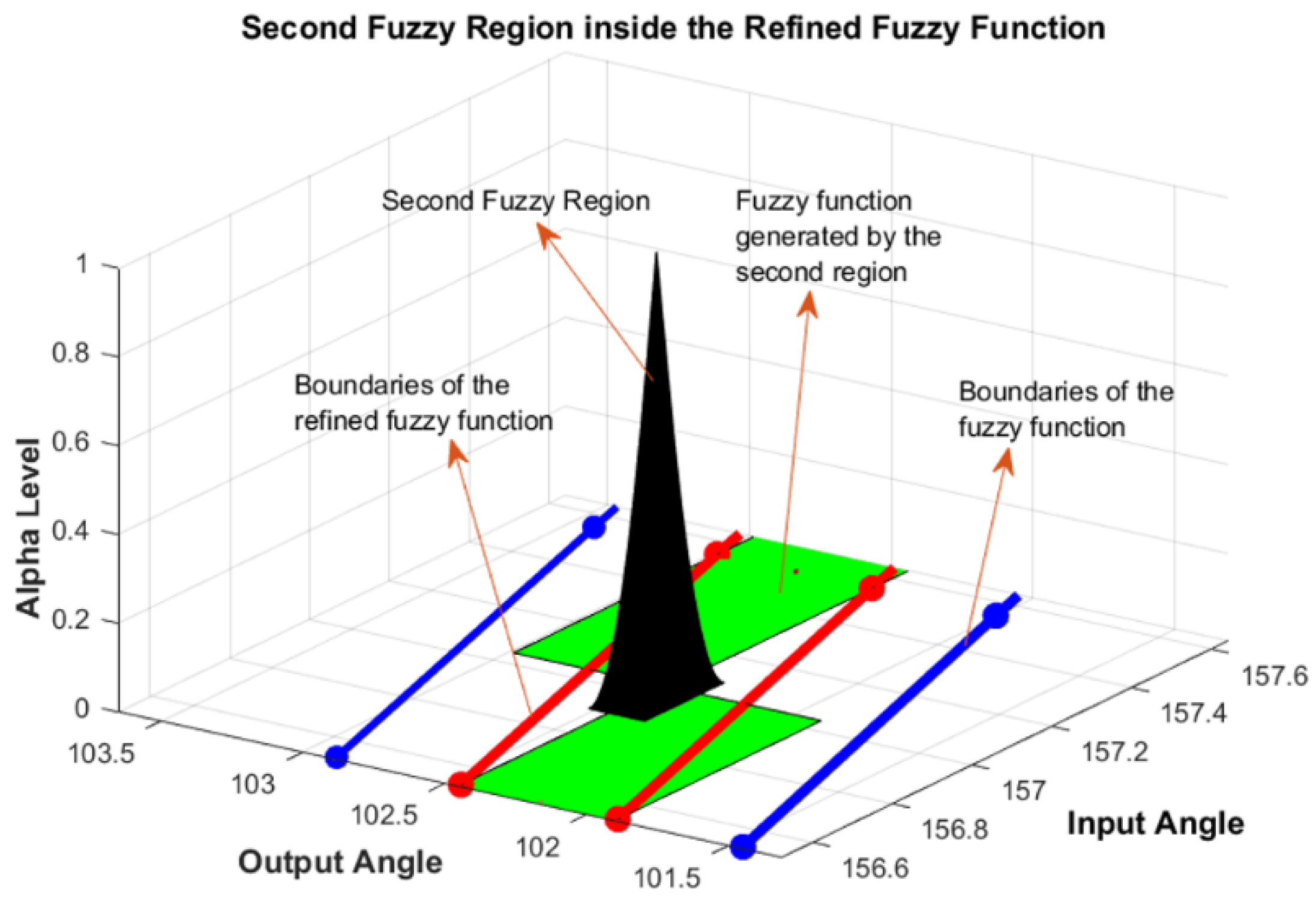
This detailed visualization highlights the way fuzzy regions and their associated fuzzy functions create a structured yet adaptable framework. This framework facilitates the understanding and optimization of compliant mechanism performance across diverse conditions. The fuzzy function expands in the areas where the alpha level is zero, as shown in the figures. The difference between the rectangular box areas and the fuzzy function represents the error of the fuzzy function. To further refine the fuzzy function, fuzzy-optimization techniques are employed. A fuzzy inference system (FIS) evaluates the error spread in the mechanism’s performance by processing multiple inputs corresponding to different error metrics calculated from the deviations between the crisp and fuzzy values at various points. These inputs are classified into categories such as “less”, “medium”, and ”more” using membership functions. The fuzzy system then applies a set of rules to combine these inputs and produce an output representing the estimated error spread.
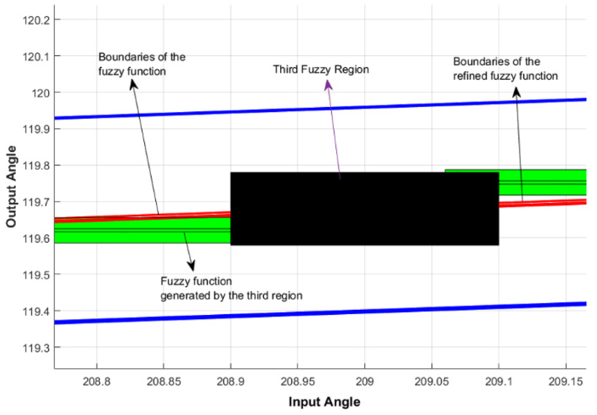
This refined fuzzy function is illustrated in Figure 22, Figure 23, Figure 24, Figure 25, Figure 26, Figure 27, Figure 28 and Figure 29, showcasing the improved accuracy and reliability of the mechanism’s performance under varying conditions. The error can be reduced by calculating the refined fuzzy regions, as shown in the figures. The rectangular green boxes of the fuzzy function and the boundaries of the fuzzy function that enclose the fuzzy regions are depicted in 3D membership functions and the X–Y frame for the zero-alpha level for all three fuzzy regions. This detailed visualization underscores how the fuzzy regions and their corresponding fuzzy functions provide a structured yet flexible framework for understanding and optimizing the performance of CMs under various conditions.

5.2. Example 2

Another CM with the same variability of the input and output angles, the constants K 1 , K 2 , and K 3 , and lengths of the crank (R2), coupler (R3), and rocker (R4) is shown in Figure 30, Figure 31, Figure 32, Figure 33, Figure 34 and Figure 35.
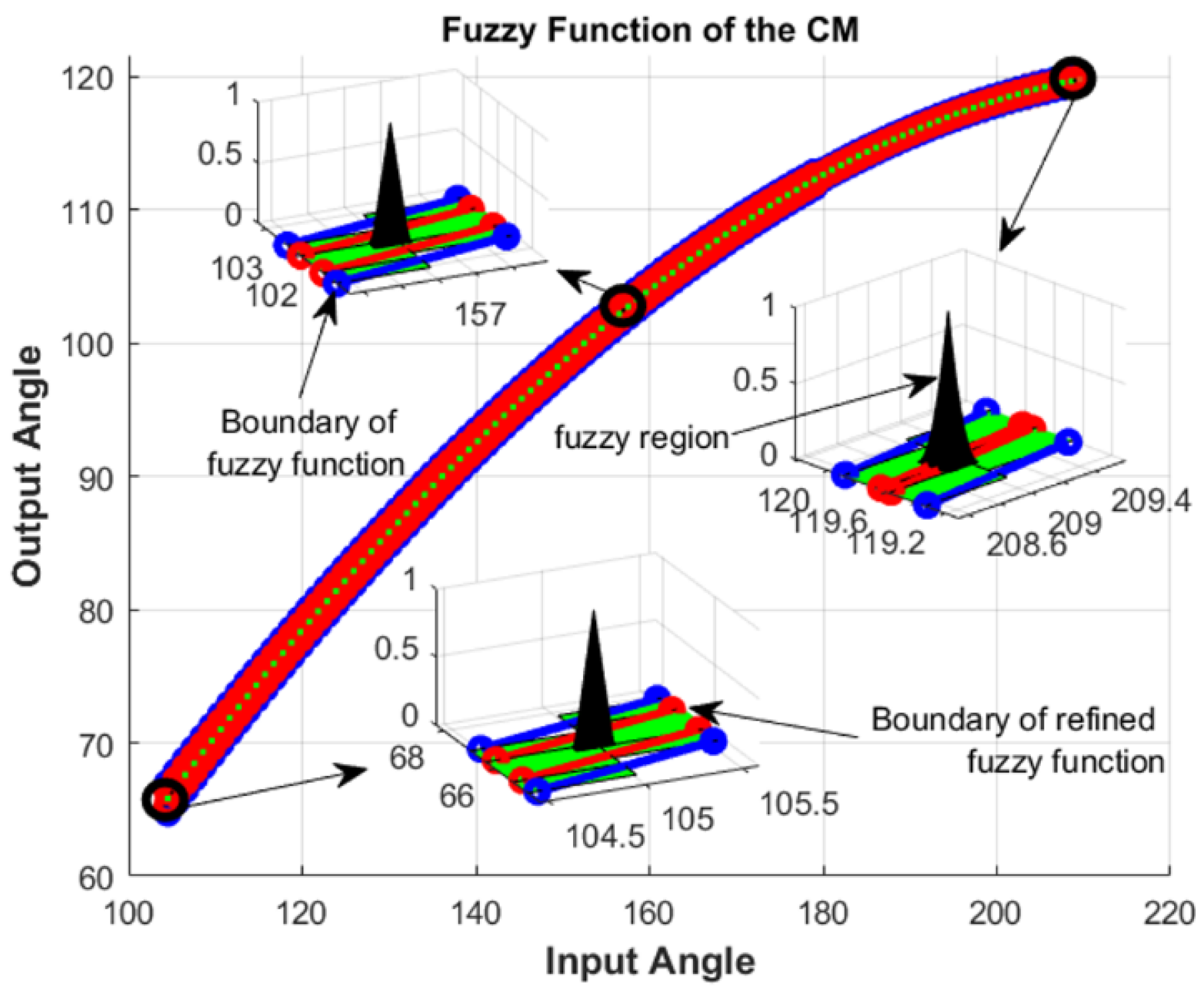
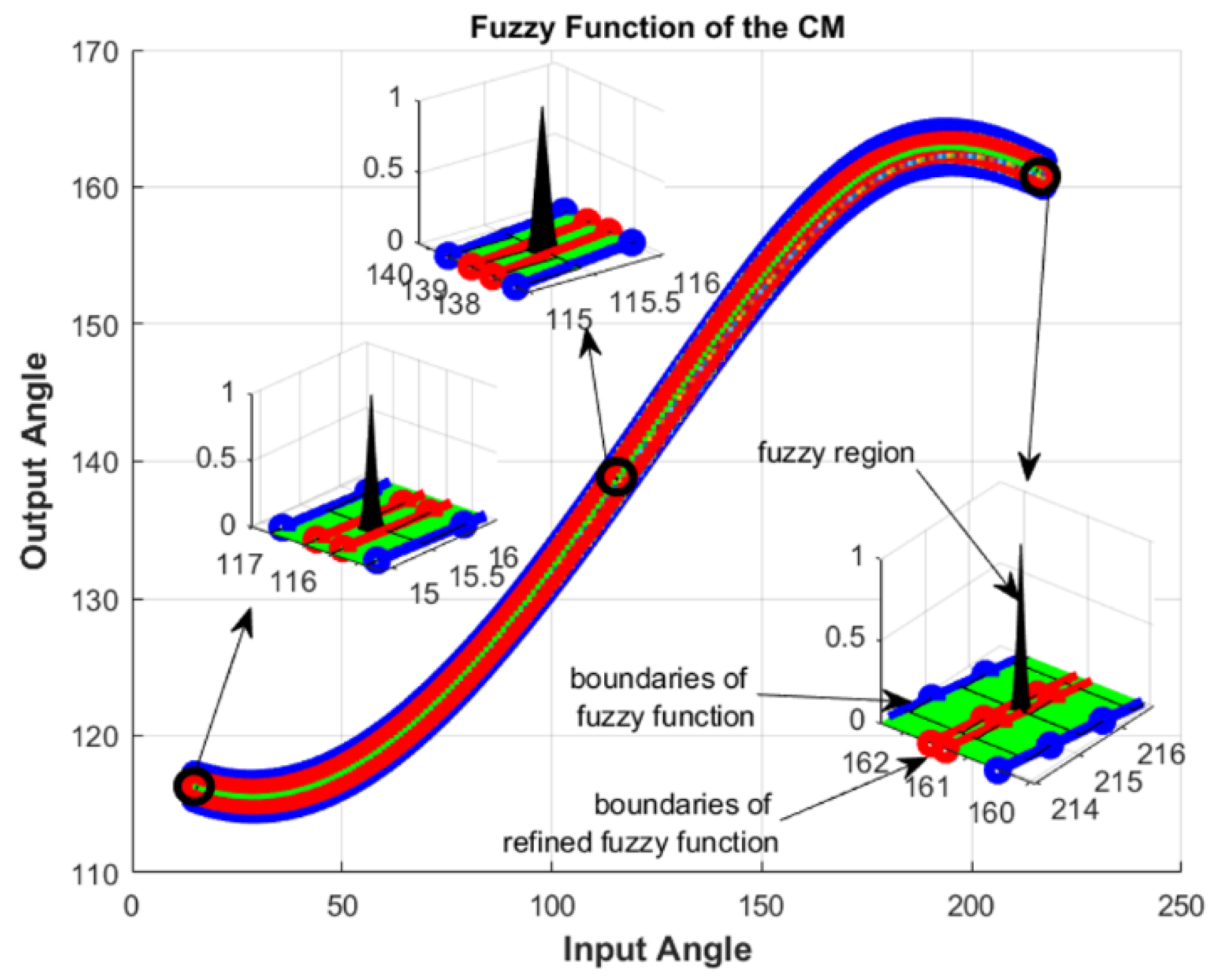
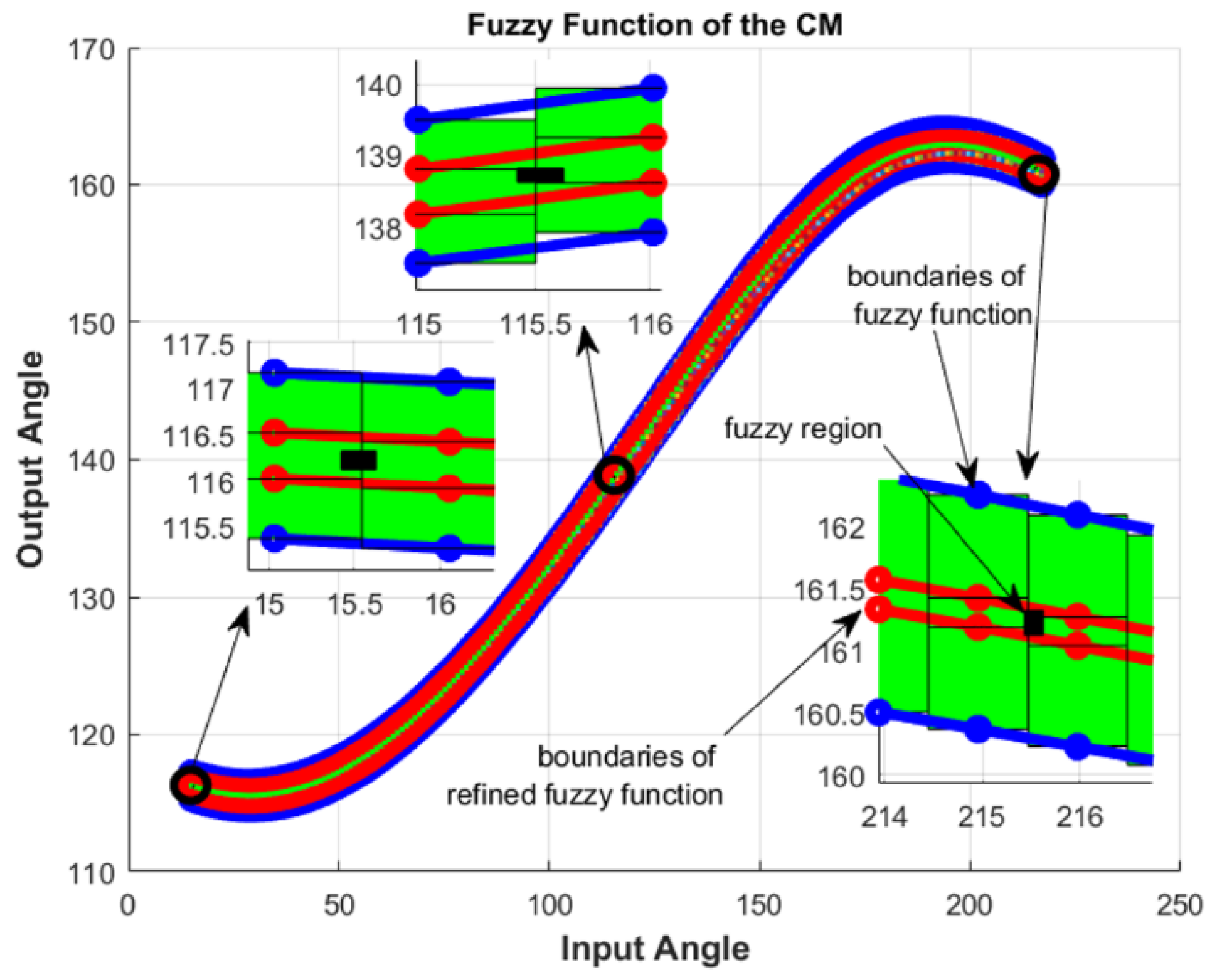
The fuzzy function of the CM that was formed by the fuzzy regions with the extended and improved boundaries is shown in Figure 36 and Figure 37.
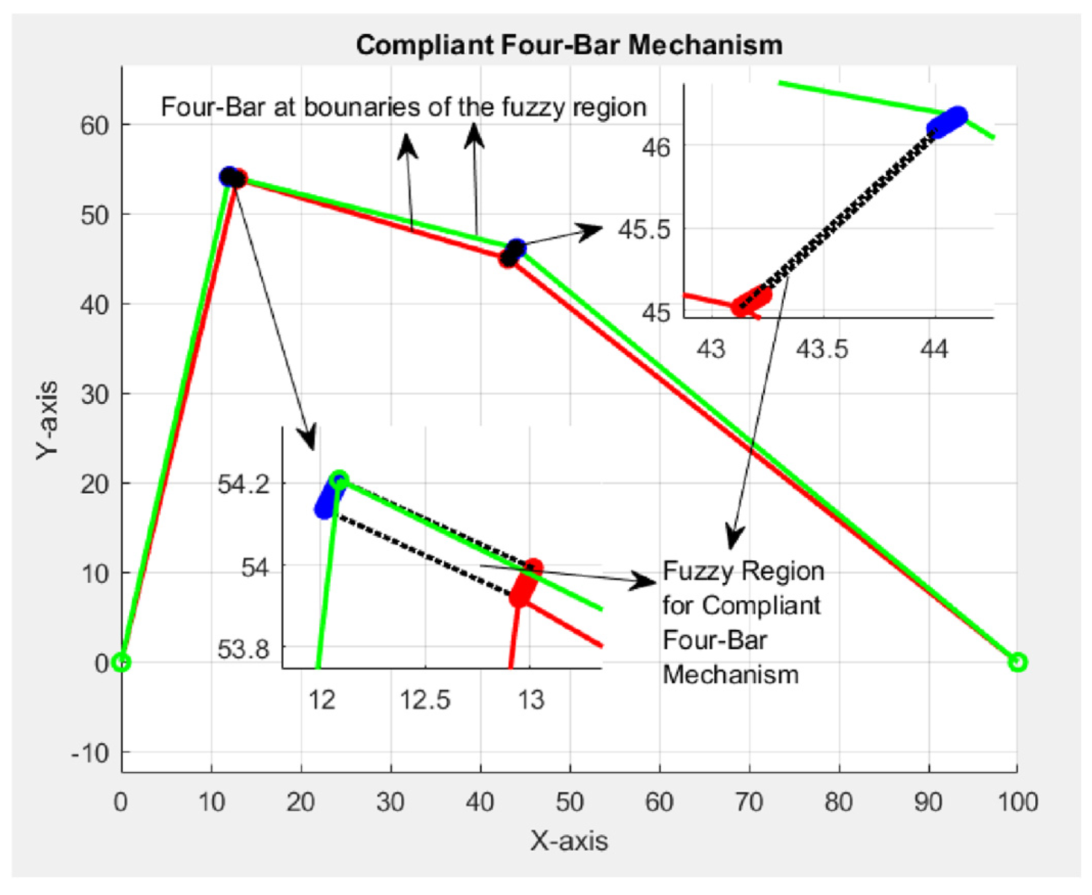
The compliant four-bar mechanism with a bounded fuzzy region in the joints that represents the possible positions for the synthesized mechanism is shown below in Figure 38.

6. Discussion

The broad range of the fuzzy function shows the mechanism’s ability to handle uncertainty. The fuzzy approach helps the mechanism adapt to variations in input parameters, like initial angles. By accounting for these uncertainties, the fuzzy function method ensures the mechanism works well across different scenarios. However, the optimization process aims to reduce the spread of these fuzzy regions. It minimizes the error between the desired and actual performance.
The refined fuzzy function, shown by the red lines in Figure 28, Figure 29, Figure 36 and Figure 37, indicates that the mechanism can still function under uncertain conditions. Yet, the optimization process has narrowed the boundaries of these fuzzy regions. In contrast, the unrefined fuzzy function, represented by green boxes and blue lines, shows a wider initial range of behaviors. This optimization leads to more precise and reliable performance, balancing flexibility with the need for accuracy in the mechanism’s design and operation.
In Figure 4, the initial four-bar CM is initiated to involve the fuzzy regions of the flexible links. Then, the fuzzy function approach is built with these fuzzy regions that have been represented as fuzzy variables. The resultant fuzzy membership functions for the lengths of the links for the four-bar CM, as shown in previous examples, have been optimized to produce the final four-bar CM shown in Figure 38. The mechanism retains its adaptability but now operates with much tighter bounds on joint positions, shown by the black bounded areas. This signifies a balance between flexibility and precision.

7. Conclusions

In conclusion, the synthesis and optimization of compliant mechanisms (CMs) using fuzzy logic principles offers a robust method for addressing the complexities and uncertainties inherent in these systems. The integration of fuzzy logic with advanced computational techniques enhances the design process, resulting in more resilient, efficient, and adaptable mechanisms. This innovative approach aligns with contemporary trends in engineering optimization and digital manufacturing, such as advanced techniques like topology optimization and genetic algorithms, highlighting the critical role of meticulous design in modern control systems to ensure accuracy and effectiveness.
However, there are certain limitations to the fuzzy function approach. For instance, when applied to complex mechanisms, the function representation can become highly complicated, making it difficult to model and optimize. Additionally, fuzzy synthesis can sometimes result in the overestimation of performance outcomes, leading to designs that may not be as effective when tested in real-world conditions.
Despite these challenges, the detailed numerical example and the refined fuzzy functions presented in this study illustrate the practical application and efficacy of the proposed methodologies. These innovations pave the way for future advancements in compliant mechanism design, balancing complexity with adaptability for optimal performance.

Author Contributions

The authors have contributed as follows: conceptualization, A.A. and M.-S.C.; methodology, A.A.; software, A.A.; validation, A.A. and M.-S.C.; formal analysis, A.A.; investigation, A.A.; writing—original draft preparation, A.A.; writing—review and editing, A.A. and M.-S.C.; supervision, M.-S.C.; project administration, M.-S.C. All authors have read and agreed to the published version of the manuscript.

Funding

This research received no funding.

Data Availability Statement

All data are contained within this article.

Acknowledgments

Thanks go to Qassim University for the support given to develop this work.

Conflicts of Interest

The authors declare no conflicts of interest.

References

  1. Howell, L.L. Compliant Mechanisms. In 21st Century Kinematics; McCarthy, J.M., Ed.; Springer: London, UK, 2013; pp. 189–216. [Google Scholar]
  2. Kota, S.; Lu, K.-J.; Kreiner, Z.; Trease, B.; Arenas, J.; Geiger, J. Design and Application of Compliant Mechanisms for Surgical Tools. J. Biomech. Eng. 2005, 127, 981–989. [Google Scholar] [CrossRef] [PubMed]
  3. Lobontiu, N. Compliant Mechanisms: Design of Flexure Hinges, 1st ed.; CRC Press: Boca Raton, FL, USA, 2002. [Google Scholar] [CrossRef]
  4. Bamberg, E. Principles of Rapid Machine Design; Massachusetts Institute of Technology: Cambridge, MA, USA, 2000; Available online: https://cir.nii.ac.jp/crid/1573105975363153536 (accessed on 23 September 2024).
  5. Howell, L.L.; Midha, A. A Method for the Design of Compliant Mechanisms with Small-Length Flexural Pivots. J. Mech. Des. 1994, 116, 280–290. [Google Scholar] [CrossRef]
  6. Su, H.-J.; McCarthy, J.M. Synthesis of Bistable Compliant Four-Bar Mechanisms Using Polynomial Homotopy. J. Mech. Des. 2006, 129, 1094–1098. [Google Scholar] [CrossRef]
  7. Hopkins, J.B.; Culpepper, M.L. Synthesis of multi-degree of freedom, parallel flexure system concepts via Freedom and Constraint Topology (FACT)–Part I: Principles. Precis. Eng. 2010, 34, 259–270. [Google Scholar] [CrossRef]
  8. Chiou, S.-J.; Sridhar, K. Automated conceptual design of mechanisms. Mech. Mach. Theory 1999, 34, 467–495. [Google Scholar] [CrossRef]
  9. Krishnan, G.; Kim, C.; Kota, S. An Intrinsic Geometric Framework for the Building Block Synthesis of Single Point Compliant Mechanisms. J. Mech. Robot. 2010, 3, 011001. [Google Scholar] [CrossRef]
  10. Kim, C. Design Strategies for the Topology Synthesis of Dual Input-Single Output Compliant Mechanisms. J. Mech. Robot. 2009, 1, 041002. [Google Scholar] [CrossRef]
  11. Bendsoe, M.P.; Sigmund, O. Topology Optimization: Theory, Methods, and Applications; Springer: Berlin/Heidelberg, Germany, 2013; Available online: https://books.google.com/books?id=ZCjsCAAAQBAJ (accessed on 23 September 2024).
  12. Saxena, A.; Ananthasuresh, G.K. Topology Synthesis of Compliant Mechanisms for Nonlinear Force-Deflection and Curved Path Specifications. J. Mech. Des. 1999, 123, 33–42. [Google Scholar] [CrossRef]
  13. Frecker, M.I.; Ananthasuresh, G.K.; Nishiwaki, S.; Kikuchi, N.; Kota, S. Topological Synthesis of Compliant Mechanisms Using Multi-Criteria Optimization. J. Mech. Des. 1997, 119, 238–245. [Google Scholar] [CrossRef]
  14. Pedersen, C.B.W.; Buhl, T.; Sigmund, O. Topology synthesis of large-displacement compliant mechanisms. Int. J. Numer. Methods Eng. 2001, 50, 2683–2705. [Google Scholar] [CrossRef]
  15. Hernández, A.; Muñoyerro, A.; Urízar, M.; Altuzarra, O. Kinematic Analysis of a Tendon-Driven Hybrid Rigid–Flexible Four-Bar; Application to Optimum Dimensional Synthesis. Mathematics 2023, 11, 4215. [Google Scholar] [CrossRef]
  16. Abbasbandy, S.; Asady, B. Newton’s method for solving fuzzy nonlinear equations. Appl. Math. Comput. 2004, 159, 349–356. [Google Scholar] [CrossRef]
  17. Todorov, T.S. Synthesis of four-bar mechanisms by Freudenstein–Chebyshev. Mech. Mach. Theory 2002, 37, 1505–1512. [Google Scholar] [CrossRef]
  18. Tanaka, H.; Watada, J. Possibilistic linear systems and their application to the linear regression model. Fuzzy Sets Syst. 1988, 27, 275–289. [Google Scholar] [CrossRef]
  19. Chukhrova, N.; Johannssen, A. Fuzzy regression analysis: Systematic review and bibliography. Appl. Soft Comput. 2019, 84, 105708. [Google Scholar] [CrossRef]
  20. Nasrabadi, M.M.; Nasrabadi, E. A mathematical-programming approach to fuzzy linear regression analysis. Appl. Math. Comput. 2004, 155, 873–881. [Google Scholar] [CrossRef]
  21. Kao, C.; Chyu, C.-L. A fuzzy linear regression model with better explanatory power. Fuzzy Sets Syst. 2002, 126, 401–409. [Google Scholar] [CrossRef]
  22. Liu, X.; Chen, Y. A systematic approach to optimizing value for fuzzy linear regression with symmetric triangular fuzzy numbers. Math Probl. Eng. 2013, 2013, 210164. [Google Scholar] [CrossRef]
  23. Chen, L.-H.; Nien, S.-H. A new approach to formulate fuzzy regression models. Appl. Soft Comput. 2020, 86, 105915. [Google Scholar] [CrossRef]
  24. Mwangi, J.K.; Muvengei, O.M.; Oduori, M.F. Review of the Application of Genetic Algorithm and Precision Points in Optimisation of the Four-bar Mechanism. In Proceedings of the Sustainable Research and Innovation Conference, Pretoria, South Africa, 22–24 June 2022; pp. 203–212. [Google Scholar]
  25. Ross, T.J. Fuzzy Logic with Engineering Applications; Wiley: Hoboken, NJ, USA, 2005. [Google Scholar]
  26. Shrestha, R.R.; Bárdossy, A.; Nestmann, F. Analysis and propagation of uncertainties due to the stage–discharge relationship: A fuzzy set approach. Hydrol. Sci. J. 2007, 52, 595–610. [Google Scholar] [CrossRef]
  27. Zadeh, L.A. Fuzzy sets. Inf. Control. 1965, 8, 338–353. [Google Scholar] [CrossRef]
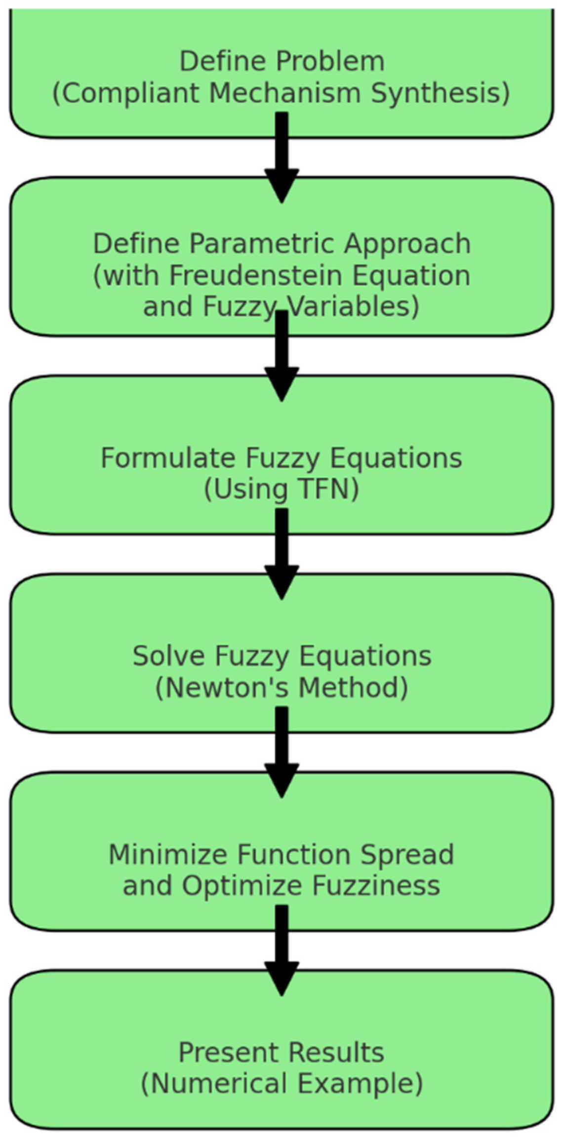
Figure 1. Process flow of the proposed synthesis of CMs.
Mathematics 12 03170 g001
Figure 2. Core, support, and boundaries of the fuzzy number.
Mathematics 12 03170 g002
Figure 3. Alpha level A α for the fuzzy number A.
Mathematics 12 03170 g003
Figure 4. The compliant mechanism (CM).
Mathematics 12 03170 g004
Figure 5. The fuzzy region of the CM.
Mathematics 12 03170 g005
Figure 6. X–Z view of a fuzzy point.
Mathematics 12 03170 g006
Figure 7. Y–Z view of the fuzzy point.
Mathematics 12 03170 g007
Figure 8. The fuzzy region.
Mathematics 12 03170 g008
Figure 9. The fuzzy rules of FISs.
Mathematics 12 03170 g009
Figure 10. First fuzzy region.
Mathematics 12 03170 g010
Figure 11. Second fuzzy region.
Mathematics 12 03170 g011
Figure 12. Third fuzzy region.
Mathematics 12 03170 g012
Figure 13. K1.
Figure 13. K1.
Mathematics 12 03170 g013
Figure 14. K2.
Figure 14. K2.
Mathematics 12 03170 g014
Figure 15. K3.
Figure 15. K3.
Mathematics 12 03170 g015
Figure 16. Length of the crank link.
Mathematics 12 03170 g016
Figure 17. Length of the coupler link.
Mathematics 12 03170 g017
Figure 18. Length of the follower link.
Mathematics 12 03170 g018
Figure 19. The fuzzy function at first fuzzy region.
Mathematics 12 03170 g019
Figure 20. The fuzzy function at second fuzzy region.
Mathematics 12 03170 g020
Figure 21. The fuzzy function at third fuzzy region.
Mathematics 12 03170 g021
Figure 22. The refined fuzzy function at first fuzzy region.
Mathematics 12 03170 g022
Figure 23. The X–Y plane of refined fuzzy function at first fuzzy region.
Mathematics 12 03170 g023
Figure 24. The refined fuzzy function at second fuzzy region.
Mathematics 12 03170 g024
Figure 25. The X–Y plane of refined fuzzy function at second fuzzy region.
Mathematics 12 03170 g025
Figure 26. The refined fuzzy function at third fuzzy region.
Mathematics 12 03170 g026
Figure 27. The X–Y plane of refined fuzzy function at third fuzzy region.
Mathematics 12 03170 g027
Figure 28. The fuzzy function of the CM at all three fuzzy regions.
Mathematics 12 03170 g028
Figure 29. The fuzzy function of the CM at all three fuzzy regions in X–Y plane.
Mathematics 12 03170 g029
Figure 30. K1.
Figure 30. K1.
Mathematics 12 03170 g030
Figure 31. K2.
Figure 31. K2.
Mathematics 12 03170 g031
Figure 32. K3.
Figure 32. K3.
Mathematics 12 03170 g032
Figure 33. The length of the crank link.
Mathematics 12 03170 g033
Figure 34. The length of the coupler link.
Mathematics 12 03170 g034
Figure 35. The length of the follower link.
Mathematics 12 03170 g035
Figure 36. The fuzzy function of the CM at all three fuzzy regions.
Mathematics 12 03170 g036
Figure 37. The fuzzy function of the CM at all three fuzzy regions in X–Y plane.
Mathematics 12 03170 g037
Figure 38. The fuzzy-optimized four-bar CM.
Mathematics 12 03170 g038
Table 1. Comparison between GAs and fuzzy function approach.
Comparison MetricGenetic Algorithms (GAs)Fuzzy Function Approach
Population InitializationRely on random sampling, which may lead to poor representation of the search space. Uniform or biased sampling can be used to improve initial population distribution [24].Not required, as fuzzy function approach naturally incorporates variability and uncertainty into the design.
Infeasibility and Illegal SolutionsMay produce infeasible or illegal solutions during the search process, requiring penalty functions or repair techniques to correct [24].Fuzzy function approach inherently accommodates a range of possible solutions due to fuzzy variable definitions, reducing the chance of infeasibility.
Sensitivity to ParametersHighly sensitive to choices like population size, mutation rate, and crossover rate, leading to potential issues with nonconvergence or suboptimal results [24].Less sensitive to such parameters because it operates within a tolerance range of solutions, making it more adaptable to changes.
Robustness to UncertaintyLimited robustness, as GAs optimize for specific parameters. Small variations in input conditions or link lengths can degrade performance [24].Designed to be robust to uncertainty in link lengths, input angles, and forces. Fuzzy synthesis accounts for variations, making the mechanism more adaptable to real-world conditions.
Optimization EfficiencyRequire careful tuning of genetic operators to achieve global optima, which can take time and multiple generations. Convergence can be slow in complex design spaces [24].Faster in scenarios involving uncertainty, as it does not need to evolve a population. Instead, it optimizes within a fuzzy range of solutions.
Disclaimer/Publisher’s Note: The statements, opinions and data contained in all publications are solely those of the individual author(s) and contributor(s) and not of MDPI and/or the editor(s). MDPI and/or the editor(s) disclaim responsibility for any injury to people or property resulting from any ideas, methods, instructions or products referred to in the content.