A Time Series Synthetic Control Causal Evaluation of the UK’s Mini-Budget Policy on Stock Market

Abstract

In this paper, we propose a modified synthetic control causal analysis for time series data with volatility in terms of absolute value of return outcomes taken into account in constructing the prediction of potential outcomes for time series causal analysis. The consistency property of the synthetic weight parameter estimators is developed theoretically under a time series data-generating process framework. The application to evaluate the UK’s mini-budget policy, announced by the then Chancellor on 23 September 2022, which had significant implications for the stock market, is examined and analysed. Comparisons with traditional synthetic control and synthetic difference in difference (DID) methods for evaluation of the effect of the mini-budget policy on the UK’s stock market are also discussed.

1. Introduction

Causal inference of the impact of a governmental policy on the financial market is important not only for evaluating the policy’s effects but also for understanding the market movement. In this study, we are interested in investigating the synthetic control method [1] in estimating the effect of the mini-budget policy by the Truss government on the UK’s stock market. This policy was announced by the then Chancellor of the Exchequer in a Ministerial Statement entitled “The Growth Plan” to the House of Commons on 23 September 2022, widely referred to in the media as a mini-budget. It contained a set of economic policies and tax cuts such as a planned cut in the basic rate of income tax from 20% to 19%, an abolition of the highest (45%) rate of income tax in England, Wales and Northern Ireland, reversing a plan of March 2021 to increase corporation tax from 19% to 25% from April 2023 and the April 2022 increase in National Insurance, and cancelling the proposed Health and Social Care Levy (according to a Wikipedia paper “September 2022 United Kingdom mini-budget” extracted on 27 May 2024). Owing to widespread negative response to the mini-budget, the planned abolition of the 45% tax rate was reversed 10 days later, and the plans to cancel the increase in corporation tax were 21 days later. In order to assess the mini-budget policy effects on the financial market, we will utilise the FTSE100 index as an aggregated dataset of the UK stocks, a good metric to reflect the UK stock market. We can therefore learn the causal effect of the mini-budget on the UK stock market by investigating how the FTSE is affected by this policy. In view of the fact that the policy was only implemented briefly in the UK, it may probably be reasonable to see that the stock indexes from other countries were not significantly affected by this policy. In this situation, the FTSE100, a share index of the 100 companies listed on the London Stock Exchange with the highest market capitalisation, may be reasonably seen as the only index affected by the mini-budget policy among the indexes from different countries in this analysis. Therefore, the synthetic control method looks like a suitable tool in solving such a problem through reasonably synthesizing the indexes from other countries to estimate the potential outcomes of the FTSE100 as the treated unit in the absence of the treatment of the mini-budget policy in the UK.

In the realm of predictive modeling for time series data, great progress has been achieved in the recent years especially in the field of predictive statistical and machine learning methods, which perform well in estimating the outcomes that are of interest given relative characteristics. However, prediction is not a causation in general. Researchers have become increasingly interested in the causal mechanism between covariates and outcomes. For example, people care about “why it happens” in addition to “what will happen”. This kind of causal mechanism help people not only to summarise a past event but also to improve the prediction accuracy of the outcomes under the varying degrees of influence of certain factors and then further help people make their decisions on the future. Evaluating the effect of some given intervention is one of the popular causal inference problems, and receives widespread attention from researchers for independent data (or for data assumed to be independent); see, e.g., Künzel et al., 2019 [2] and Wager and Athey, 2018 [3]. However, the causal effect evaluation for time series data is the problem that is of our interest in this paper. There remain few investigating time series causal evaluations apart from interrupted time series analysis (c.f. [4]). For more discussions with relevant references, see [5], where causal inference for time series is seen as a (counterfactual) prediction problem built on the literature on conformal prediction.

The synthetic control method (SCM) has been popular, and is called “arguably the most important innovation in the last 15 years” (Anthey and Imbends, 2017 [6]) in evaluating the effect of some given treatment on a single unit (Abadie et al., 2010 [1]). It makes use of the control units to construct the potential outcomes of the treated unit after intervention by weighted averaging of the outcomes of the control units. The weights, referred to as synthetic weights, are determined by minimising the difference between the synthetic series and the observed treated series before intervention. Then, the causal effect of the given treatment is estimated to be the difference between the observed series of the treated unit and the synthetic series after the treatment time.

Conventional SCM constructs the potential outcome series which has similar characteristics to the observed treated unit in terms of not only the pre-intervention outcomes but also the covariates that could affect the outcomes. In this way, the effect of confounding factors that possibly confound the causal effect estimation can be effectively eliminated under suitable assumptions. However, considering that the SCM is usually applied in a setting associated with time, it is reasonable for us to take time series properties into consideration as some “time series covariates” while determining the synthetic weights to improve the performance of the conventional SCM. Generally, the conventional SCM has considered all the pre-intervention outcomes, which could have been seen as involving the lagged outcomes when determining the synthetic weights. This property of the SCM could make synthetic outcome series automatically include the autocorrelation properties of the observed outcome series. We will show this property of the SCM in our empirical study. However, in addition to autocorrelation, conditional heteroskedasticity, which is especially widespread in financial time series data, is also an important characteristic and should be taken into account when determining the synthetic weights. Therefore, in this paper, we propose a modified synthetic control method (MSCM) to help cover the conditional heteroskedasticity of the original treated series to improve the performance of the conventional SCM in causal effect inference and compare its performance with the conventional SCM in the empirical study to evaluate the causal effect of the mini-budget policy in the UK.

Our modified synthetic control method, on the one hand, improves the estimation accuracy for the potential outcome series, when compared to the conventional synthetic control method. We will demonstrate this by the pre-intervention mean squared error (MSE) of the two methods. In our empirical study, the MSE of our modified synthetic control method is shown to decrease by 40% compared with the conventional synthetic control method, which significantly illustrates the improvement of the modified synthetic control method. On the other hand, by considering the volatility in terms of absolute return in the empirical study, the pre-intervention residuals by the modified synthetic control method are well controlled to have a stable fluctuation degree. This implies that the residual series produced by the modified synthetic control has a stable variance while through the conventional synthetic control method the residual series are obviously heteroskedastic as shown in Section 4.3. Thus, we can reasonably assume that the residuals along time have the homoskedasticity property by our modified synthetic control method. Therefore, we can establish the consistency of the estimated synthetic weights by the modified synthetic control method; thus, the consistency of the estimated potential outcomes is naturally achieved under weaker assumptions than Chernozhukov et al. [5]. Note that Chernozhukov et al. [5] achieve the consistency of the potential outcome estimations under more stringent assumptions due to violation of homoskedasticity of the residual series.

The structure of the rest of this paper is as follows. Section 2 introduces the preliminaries for causal analysis, including notations, a potential outcome-based causal framework and the conventional synthetic control method. In Section 3, we propose the modified synthetic control method including its overview, the form of the model and the consistency of the estimated synthetic weights. Section 4 will apply our new method to an empirical study, which evaluates the causal effect of the mini-budget policy on the UK’s stock market. We will demonstrate the performance of the modified synthetic control method proposed by this paper by comparing our method to the conventional synthetic control method and the synthetic difference in difference method popular in the causal evaluation literature. Finally, Section 5 presents the conclusion. The theoretical proof of the consistency property will be relegated to Appendix A.

2. Preliminaries of Causal Analysis

In this section, we introduce preliminaries on the potential outcome causal framework, which is applied in this paper, due to Neyman [7] and Rubin (c.f., the synthetic control method proposed by Abadie et al. [1]).

2.1. Notations

We consider the panel data $Y_{it}$, a type of data collected for units, $i=1,\cdots ,J+1$, observed over a period of time at a regular frequency, $t=1,\cdots ,T$. The indicator of a treatment assignment is defined to be a binary $W_{it}$ for unit i at time t, where $W_{it}=0$ stands for unit i not to be under the treatment at time t while $W_{it}=1$ implies that the unit i is under the treatment at time t. Further, suppose the intervention time is at time $T_0$ ($1<T_0<T$); that is, after the time $T_0$, a group of units, called treated units, are assigned the treatments, while the rest, called control units, will remain untreated over the period. This hence implies that $W_{it}=1$ for a treated unit i, while $W_{it}=0$ for a non-treated unit i, at $t>T_0$. In synthetic control casual effect evaluation problems, we are often interested in the situation where only one or a few units are affected by the intervention. Without loss of generality, we let unit 1 be the only treated unit and others the control units, the number of which is hence J. Moreover, as we care about only the effect of a given intervention, the treatment assignment is binary and there are only two potential outcomes for unit i at time t, which are denoted by $Y_{it}^{\left(0\right)}$ in the absence of the treatment and $Y_{it}^{\left(1\right)}$ under the treatment, respectively. In addition, the observed outcome of unit i at time t is denoted by $Y_{it}$ and the vector of p observed covariates for unit i at time t by ${\mathbf{Z}}_{it}$. As usual, we will denote the causal effect by $\tau$, defined specifically below.

2.2. Causal Framework

We introduce the needed potential outcome causal framework, based on which the synthetic control method and our modified synthetic control method are conceptually defined. Note that in causal inference problem, data of the control units after the intervention time $T_0$ are available for causal evaluation. This means we can make use of the data for the control units after intervention to estimate the potential outcome of the treated units. Applying the potential outcome framework due to Neyman [7] and Rubin (see, e.g., [8]), we need to posit the existence of the two potential outcomes. In the case of independent and identically distributed (i.i.d.) data across units, the average treatment effect is usually of interest. Recall that the potential outcomes at time t are denoted by $Y_{it}^{\left(0\right)}$ in the absence of treatment and $Y_{it}^{\left(1\right)}$ under the treatment, respectively. Then, in general, at $t>T_0$, the average treatment effect in population is

$${\tau }_t^{\mathrm{ave}}=E_i[Y_{i,t}^{\left(1\right)}-Y_{i,t}^{\left(0\right)}],$$

(1)

where $E_i$ denotes the average in population across the individual units i, while the individual treatment effect for unit i at time t is

$${\tau }_{it}=Y_{i,t}^{\left(1\right)}-Y_{i,t}^{\left(0\right)}.$$

(2)

When there is only one or a few units affected by the intervention, the individual treatment effect is a more suitable metric to evaluate the causal effect because the number of the treated units i is limited with the scales of the treated and the control units seriously unbalanced. Therefore, the individual causal effect of the treated unit i is of interest often in the synthetic control case.

Rubin suggested that we cannot infer the causal effect without rational assumptions that link statistics to science [9]. We thus made some assumptions to implement causal inference, including unconfoundedness assumption [10] and stable unit treatment values assumptions (SUTVA), which are wildly used for causal inference. Here, the unconfoundedness assumes that the treatment assignment $W_{it}$ is independent of the potential outcomes conditional on the vector of covariates ${\mathbf{Z}}_{it}$, often denoted by

$$\left\{Y_{it}^{\left(0\right)},Y_{it}^{\left(1\right)}\right\}⫫W_{it}|{\mathbf{Z}}_{it}.$$

(3)

The SUTVA includes no interference assumption and no hidden variations of treatment assumption. No interference means that the potential outcomes for any unit do not vary with the treatments assigned to other units, while the no hidden variation of treatment assumes that for each unit, there are no different forms or versions of each treatment level, which lead to different potential outcomes.

2.3. The Conventional Synthetic Control Method

In this section, we briefly introduce the conventional synthetic control method proposed by Abadie [1] as a benchmark method based on which we will suggest our modified synthetic control method in the next section. The synthetic control method [1] is a popular causal inference method in evaluating the causal effect of some certain intervention on the treat unit. It imputes the counterfactual by weighted averaging the outcomes of the control units. In the synthetic control method, we take unit $i=1$ for the treated unit, and other units for the control units. A useful exemplary model for the potential outcome $Y_{it}^{\left(0\right)}$ in [1] is defined by a factor model:

$$Y_{it}^{\left(0\right)}={\delta }_t+{\theta }_t{\mathbf{Z}}_i+{\lambda }_t{\mu }_i+{\epsilon }_{it},$$

(4)

where ${\mathbf{Z}}_i$ is a vector of p observable covariates and ${\mu }_i$ is a vector of unobserved factors for unit i, ${\epsilon }_{it}$ is a zero mean error term, and ${\theta }_t$ and ${\lambda }_t$ are the time-varying coefficients. The weights for the control units, which are called the synthetic weights, are determined through balancing the properties of the units under or in the absence of the treatment before the intervention. Suppose there exist $(w_2^{*},\dots ,w_{J+1}^{*})$ such that

$$\sum _{j=2}^{J+1}{w}_j^{*}{Y}_{j1}=Y_{11},\sum _{j=2}^{J+1}{w}_j^{*}{Y}_{j2}=Y_{12},\dots ,\sum _{j=2}^{J+1}{w}_j^{*}{Y}_{j{T}_0}=Y_{1T_0}\mathrm{and}\sum _{j=2}^{J+1}{w}_j^{*}{\mathbf{Z}}_j={\mathbf{Z}}_1.$$

(5)

In general, it is impossible to do as indicated in (5), so what we are trying to do is to find a series of weights $\widehat{\mathsf{\omega }}={({\widehat{w}}_2,\dots ,{\widehat{w}}_{J+1})}^{\prime }$ close to the weights $w_j^{*}$ by approximation to solve the equation:

$$\widehat{\mathsf{\omega }}=arg\underset{\mathsf{\omega }}{min}\left|\right|{\mathbf{V}}_{\mathbf{x}}^{1/2}({\mathbf{X}}_{\mathbf{1}}-{\mathbf{X}}_{\mathbf{0}}\mathsf{\omega }){\left|\right|}_2^2=:{({\mathbf{X}}_{\mathbf{1}}-{\mathbf{X}}_{\mathbf{0}}\mathsf{\omega })}^{\prime }{\mathbf{V}}_{\mathbf{x}}({\mathbf{X}}_{\mathbf{1}}-{\mathbf{X}}_{\mathbf{0}}\mathsf{\omega }),$$

(6)

where $\left|\right|·{\left|\right|}_2$ stands for the $L_2$ Euclidean norm, $\mathsf{\omega }={(w_2,...,w_{J+1})}^{\prime }$, with the notation $\prime$ in the superscript denoting the transpose of a vector or matrix, satisfies ${\displaystyle \sum _{i=2}^{J+1}}{w}_i=1$ and $w_i\ge 0$ for $2\le i\le J+1$, ${\mathbf{X}}_{\mathbf{1}}$ is the vector that contains the pre-treatment outcomes $Y_{1t}$, $1\le t\le T_0$, and observable covariate ${\mathbf{Z}}_1$ for the treated unit, and ${\mathbf{X}}_{\mathbf{0}}$ is a $(T_0+p)\times J$ matrix whose j-th column vector contains the corresponding pre-treatment outcomes $Y_{jt}$, $1\le t\le T_0$, and observable covariate vector ${\mathbf{Z}}_j$ for the control units, with p denoting the dimension of the vector ${\mathbf{Z}}_i$. Here, ${\mathbf{V}}_{\mathbf{x}}\in {\mathbb{R}}^{(T_0+p)\times (T_0+p)}$ is a pre-specified symmetric importance matrix which grants different importance weights to the properties specified in (5) for the units. To simplify the exposition and notation, ${\mathbf{V}}_{\mathbf{x}}$ is set to be an identity matrix, that is with equal importance weight for each equation in (5), in this paper as Ben-Michael et al. [11] did.

After the synthetic weights are determined as above, the potential outcomes of the treated unit in the absence of the treatment can be estimated through the weighted averaging of the observed outcomes of the control units:

$${\widehat{Y}}_{1t}^{\left(0\right)}=\sum _{i=2}^{J+1}{\widehat{w}}_i{Y}_{it}\mathrm{for}t>T_0.$$

(7)

Then, the causal effect of the intervention can be derived by comparing the estimated potential with the observed outcomes of the treated unit, by noting that $Y_{1t}^{\left(1\right)}=Y_{1t}$ for $t>T_0$,

$${\widehat{\tau }}_t=Y_{1t}-{\widehat{Y}}_{1t}^{\left(0\right)},t>T_0.$$

(8)

3. The Modified Synthetic Control Method

As introduced in the last section, the synthetic control method determines the synthetic weights by balancing the outcomes $Y_{it}$ and covariates ${\mathbf{Z}}_i$ of the units under or in the absence of the treatment before intervention time. In our real data example on mini-budget impact below, $Y_{it}$ is the daily stock market return series with unit i standing for individual country, and ${\mathbf{Z}}_{it}$ is the interest rate of the corresponding country i but depending on time t. It is a well known fact that the volatility of the stock-return series is often clustered; that is, while returns themselves are uncorrelated, absolute returns or their squares display a positive, significant and slowly decaying auto-correlation function [12], which is however not taken into account by the conventional synthetic control method. We have hence followed Granger and Ding [13] with the absolute return value seen as a local volatility measure. In this section, we hence suggest a modified synthetic control method which additionally considers the absolute value of the outcomes, standing for their local volatility. Thus, in addition to the lagged terms of the outcome, as mentioned by Abadie [1], the absolute value of the outcomes should also be taken into consideration while applying the synthetic control method on interrupted time series problems [4], especially for financial time series. Because there usually exists conditional heteroskedasticity in such time series as a very important characteristic, ignoring it might affect the quality of the synthetic counterfactual series. We will show the improvement of the modified synthetic control method over the conventional synthetic control method through the empirical study in next section.

3.1. Form of the Modified Synthetic Control Method

For convenience, we have made the variables centralised with mean zero in discussion of the modified synthetic control method, designed to infer the causal effect of an intervention on series in time. We consider zero-mean stationary series $Y_{jt}$ for units $j=1,2,\cdots ,J+1$, in which the absolute value of these outcomes would be helpful and reasonable, with unit $j=1$ for the treated unit and others for the control units. Specifically, we suppose there are a series of weights $(w_2^{*},\dots ,w_{J+1}^{*})$ that could make

$$\begin{array}{cc}\hfill & \sum _{j=2}^{J+1}{w}_j^{*}{Y}_{j1}=Y_{11},\sum _{j=2}^{J+1}{w}_j^{*}{Y}_{j2}=Y_{12},\cdots ,\sum _{j=2}^{J+1}{w}_j^{*}{Y}_{j{T}_0}=Y_{1T_0},\hfill \\ \hfill & \sum _{j=2}^{J+1}{w}_j^{*}|Y_{j1}|=|Y_{11}|,\sum _{j=2}^{J+1}{w}_j^{*}|Y_{j2}|=|Y_{12}|,\cdots ,\sum _{j=2}^{J+1}{w}_j^{*}|Y_{j{T}_0}|=|Y_{1T_0}|,\hfill \\ \hfill & \mathrm{and}\sum _{j=2}^{J+1}{w}_j^{*}{\mathbf{Z}}_{j1}={\mathbf{Z}}_{11},\sum _{j=2}^{J+1}{w}_j^{*}{\mathbf{Z}}_{j2}={\mathbf{Z}}_{12},\cdots ,\sum _{j=2}^{J+1}{w}_j^{*}{\mathbf{Z}}_{j{T}_0}={\mathbf{Z}}_{1T_0},\hfill \end{array}$$

(9)

hold. Then, we try to find a series of weights $\widehat{\mathsf{\omega }}=({\widehat{w}}_2,\dots ,{\widehat{w}}_{J+1})$ close to the weights $w_j^{*}$ by approximation to solve:

$$\widehat{\mathsf{\omega }}=\underset{\begin{array}{c}{w}_2,\dots ,w_{J+1}\ge 0,\\ {\displaystyle \sum _{j=2}^{J+1}}{w}_j=1\end{array}}{argmin}\sum _{t=1}^{T_0}\left\{v_1{(Y_{1t}-\sum _{j=2}^{J+1}{\omega }_j{Y}_{jt})}^2+v_2\left(\right|Y_{1t}{|-\sum _{j=2}^{J+1}{\omega }_j\left|Y_{jt}\right|)}^2+\sum _{k=1}^p{v}_{i+2}{(Z_{1t}^{\left(k\right)}-\sum _{j=2}^{J+1}{\omega }_j{Z}_{jt}^{\left(k\right)})}^2\right\},$$

(10)

where $Z_{jt}^{\left(k\right)}$ represents for the k-th covariate of ${\mathbf{Z}}_{jt}$ for unit j at time t, $k=1,\cdots ,p$, and $v_1,v_2,\cdots ,v_{p+2}$ are the pre-specified group importance weight coefficients for each row group in (9), in the same spirit (but a special case) of the importance matrix ${\mathbf{V}}_{\mathbf{x}}$ in (6), which reflect the relative importance of the synthetic control reproducing the values for each type of the predictors in (9) for the treated unit (Abadie, 2021 [14]). In the following, all those v’s are just taken as 1 for simplicity and ease. Then, similarly to the conventional synthetic control method, after estimating the synthetic weights, the potential outcomes of the treated unit $i=1$ in the absence of the treatment can be estimated by:

$${\widehat{Y}}_{1t}^{\left(0\right)}=\sum _{i=2}^{J+1}{\widehat{w}}_i{Y}_{it}\mathrm{for}t>T_0,$$

(11)

following from which the estimated causal effect of the intervention at time $t>T_0$ is:

$${\widehat{\tau }}_t=Y_{1t}-{\widehat{Y}}_{1t}^{\left(0\right)}.$$

(12)

The consistency property of such an estimator is given in the next subsection. In Section 4, we test its performance in an empirical study and compare it with the conventional synthetic control method.

3.2. Consistency of the Modified Synthetic Control Method

In terms of the theoretical results of the synthetic control method, some work has been carried out for the estimated potential outcomes. Abadie et al. [1] proved that the bias of the synthetic control estimator can be bounded by a function that goes to zero as the number of pre-treatment periods increases. Chernozhukov et al. [5] regard the conventional synthetic control estimator, which only considers the outcomes of the units, as a constrained least squares estimator and give the consistency of the estimated potential outcomes. Despite these existing theories for the estimated potential outcomes, researchers seldom focus on the limiting theorems of the synthetic weights, which are essential in synthetic-type methods. Therefore, we tend to give the consistency property of the synthetic weights of the modified synthetic control method which considers the absolute outcomes and the relevant covariates, to fill this gap.

Like Chernozhukov et al. [5], we regard the synthetic control estimator as a constrained least squared estimator, i.e., the non-negative least square estimator. Correspondingly to (9), we define

$${\mathbf{Y}}_{\mathbf{1}\mathbf{t}}^{\left(\mathbf{0}\right)}=(Y_{1t},|Y_{1t}{|,Z_{1t}^{\left[1\right]},Z_{1t}^{\left[2\right]},\dots ,Z_{1t}^{\left[p\right]})}^{\prime },$$

$${\mathbf{X}}_{\mathbf{t}}^{\left(\mathbf{0}\right)}=\left(\begin{array}{cccc}{Y}_{2t}& Y_{3t}& \dots & Y_{J+1t}\\ |Y_{2t}|& |Y_{3t}|& \dots & |Y_{J+1t}|\\ Z_{2t}^{\left[1\right]}& Z_{3t}^{\left[1\right]}& \dots & Z_{J+1t}^{\left[1\right]}\\ ⋮& ⋮& ⋮& ⋮\\ Z_{2t}^{\left[p\right]}& Z_{3t}^{\left[p\right]}& \dots & Z_{J+1t}^{\left[p\right]}\end{array}\right),$$

$$\mathsf{\omega }={(w_2,w_3,\dots ,w_{J+1})}^{\prime }$$

and

$${\mathsf{\epsilon }}_t=({\epsilon }_t\left(Y\right),{\epsilon }_t\left(\right|Y\left|\right),{\epsilon }_t\left(Z^{\left[1\right]}\right),\cdots ,{\epsilon }_t\left(Z^{\left[p\right]}\right){)}^{\prime }$$

standing for the vector for the treated unit, the matrix that contains the vectors of the control units, the vector of synthetic weights and the relevant residuals, respectively. According to the equations given in (9), we have:

$${\mathbf{Y}}_{\mathbf{1}\mathbf{t}}^{\left(\mathbf{0}\right)}={\mathbf{X}}_{\mathbf{t}}^{\left(\mathbf{0}\right)}\mathsf{\omega }+{\epsilon }_t.$$

(13)

Then, the “true synthetic weights” $w^{*}$ are defined by minimising the population error:

$${\omega }^{*}=arg\underset{w\ge 0}{min}E{\parallel {\mathbf{Y}}_{\mathbf{1}\mathbf{t}}^{\left(\mathbf{0}\right)}-{\mathbf{X}}_{\mathbf{t}}^{\left(\mathbf{0}\right)}\omega \parallel }_2^2,$$

(14)

where the $L_2$ norm ${\parallel ·\parallel }_2$ of a vector $\mathbf{a}$ is defined to be ${\parallel \mathbf{a}\parallel }_2=\sqrt{{\mathbf{a}}^T\mathbf{a}}$. Note that “true synthetic weights” here refers to the population version of the weights defined by Equation (14), where the population synthetic weight vector ${\mathsf{\omega }}^{*}$ is defined by minimising the population synthetic mean squared error. This does not mean that the synthetic regression model based on the equations in (9) is true—it only means an optimal approximation in the sense that the population synthetic mean squared error in Equation (14) is minimised.

To obtain the estimated synthetic weights by non-negative regression based on the pre-intervention data ranging from $t=1$ to $t=T_0$, we define the pre-intervention observations of the treated unit to be:

$${\mathit{Y}}_{\mathbf{1}}^{\mathit{pre}}={({{\mathit{Y}}_{\mathbf{11}}^{\left(\mathbf{0}\right)}}^{\prime },{{\mathit{Y}}_{\mathbf{12}}^{\left(\mathbf{0}\right)}}^{\prime },\cdots ,{{\mathit{Y}}_{\mathbf{1}{\mathit{T}}_{\mathbf{0}}}^{\left(\mathbf{0}\right)}}^{\prime })}^{\prime }$$

(15)

and the matrix that contains pre-intervention observations of control units is:

$${\mathit{X}}_{\mathbf{0}}^{\mathit{pre}}={({{\mathbf{X}}_{\mathbf{1}}^{\left(\mathbf{0}\right)}}^{\prime },{{\mathbf{X}}_{\mathbf{2}}^{\left(\mathbf{0}\right)}}^{\prime },\cdots ,{{\mathbf{X}}_{T_0}^{\left(0\right)}}^{\prime })}^{\prime }.$$

(16)

Since all the elements in the above vector and matrix are not affected by the intervention before $T_0$, their observation values could be directly regarded as the potential outcomes. Then, based on the observation data, we can estimate the synthetic weights through:

$$\widehat{\mathsf{\omega }}=arg\underset{\mathsf{\omega }\ge 0}{min}{\displaystyle \frac{1}{T_0}}\parallel {\mathit{Y}}_{\mathbf{1}}^{\mathit{pre}}-{\mathit{X}}_{\mathbf{0}}^{\mathit{pre}}{\mathsf{\omega }\parallel }_2^2=:{\displaystyle \frac{1}{T_0}}\sum _{t=1}^{T_0}{\parallel {\mathbf{Y}}_{\mathbf{1}\mathbf{t}}^{\left(\mathbf{0}\right)}-{\mathbf{X}}_{\mathbf{t}}^{\left(\mathbf{0}\right)}\mathsf{\omega }\parallel }_2^2.$$

(17)

In application, we can then normalise the estimator $\widehat{\mathsf{\omega }}$ so that the summation of the components equals 1. The estimation of the parameters is easily implemented by using the function “Synth” of the “SyntheticControlMethods” package in Python (Version 3.8.2).

The following theorem shows that the estimator $\widehat{\mathsf{\omega }}$ is a consistent estimator of ${\mathsf{\omega }}^{*}$ as the sample size $T_0\to \infty$.

Theorem 1.

(1) Let $\left({\mathsf{\epsilon }}_{\mathit{t}}\right)$ be the error term vector ${\mathsf{\epsilon }}_t={\mathbf{Y}}_{1t}^{\left(0\right)}-{\mathbf{X}}_t^{\left(0\right)}{\mathsf{\omega }}^{*}$ that satisfies $E\left[{\mathsf{\epsilon }}_{\mathit{t}}\right]=0$, $E[\parallel {\mathsf{\epsilon }}_{\mathit{t}}{\parallel }^2]={\sigma }^2$ and $E[\parallel {\mathsf{\epsilon }}_{\mathit{t}}{\parallel }^4]<\infty$. (2) $\{{\mathbf{Y}}_{1t}^{\left(0\right)},{\mathbf{X}}_t^{\left(0\right)}\}$ is an α-mixing stationary sequence, with the mixing coefficient $\alpha \left(k\right)={sup}_{A\in {\mathcal{F}}_{-\infty }^t,B\in {\mathcal{F}}_{t+k}^{\infty }}|P\left(AB\right)-P\left(A\right)P\left(B\right)|\to 0$ as $k\to \infty$, where ${\mathcal{F}}_s^t$ stands for the σ-algebra (or intuitively an information set) of ${\{{\mathbf{Y}}_{1j}^{\left(0\right)},{\mathbf{X}}_j^{\left(0\right)}\}}_{s\le j\le t}$. (3) Let $\mathbf{v}={\mathit{X}}_{\mathbf{0}}^{\mathit{pre}}{\mathsf{\omega }}^{*}-{\mathit{X}}_{\mathbf{0}}^{\mathit{pre}}\mathsf{\omega }$, with ${\mathbf{v}}_t$ being the sub-vector of $\mathbf{v}$ corresponding to ${\mathsf{\epsilon }}_t$, and ${\displaystyle \frac{1}{T_0}}{\mathbf{v}}^{\prime }\mathsf{\epsilon }={\displaystyle \frac{1}{T_0}}{\displaystyle \sum _{t=1}^{T_0}}{\mathbf{v}}_t^{\prime }{\mathsf{\epsilon }}_t$. Further, ${\mathbf{v}}_t^{\prime }{\mathsf{\epsilon }}_t$ for $t=1,2,...$ is an α-mixing series with its mixing coefficient $\alpha \left(n\right)\le exp(-2cn)$ for a certain $c>0$. (4) There exists $M=M_{T_0}$ that satisfies ${\displaystyle \frac{M^2}{T_0}}=o\left(1\right)$ and ${\displaystyle \frac{T_0}{M^4}}=o\left(1\right)$. (5) Moreover, the minimum eigenvalue of ${\left({\mathit{X}}_{\mathbf{0}}^{\mathit{pre}}\right)}^{\prime }{\mathit{X}}_{\mathbf{0}}^{\mathit{pre}}$, denoted by ${\lambda }_{min}$, has positive lower bound ${\lambda }_{min}>C>0$. Then, $\widehat{\mathsf{\omega }}$ is a consistent estimation of ${\mathsf{\omega }}^{*}$, that is:

$$\widehat{\mathsf{\omega }}\stackrel{p}{\to }{\mathsf{\omega }}^{*},as{T}_0\to \infty .$$

Theoretically, it is hoped that an optimal approximation in (14) can be achieved to generate the synthetic regression residuals that are the least informative (i.e., more like a purely white noise) in the sample version for the estimator given by Equation (17). Clearly, the consistency of the estimator given in Equation (17) converging to the population optimal synthetic weight vector ${\mathsf{\omega }}^{*}$ is theoretically important, ensuring that the sample version estimator makes sense. Then, we can further conclude that the potential outcomes synthesised by these consistent synthetic weights are consistent estimation of the potential outcomes.

4. Evaluating the Mini-Budget Policy on UK Stock Market: An Empirical Study

In this section, we take an empirical study to compare the performance of the modified synthetic control method with the conventional synthetic control method in evaluating the causal effect of “The Growth Plan” by the Truss government, widely referred to in the media as a mini-budget.

4.1. Data

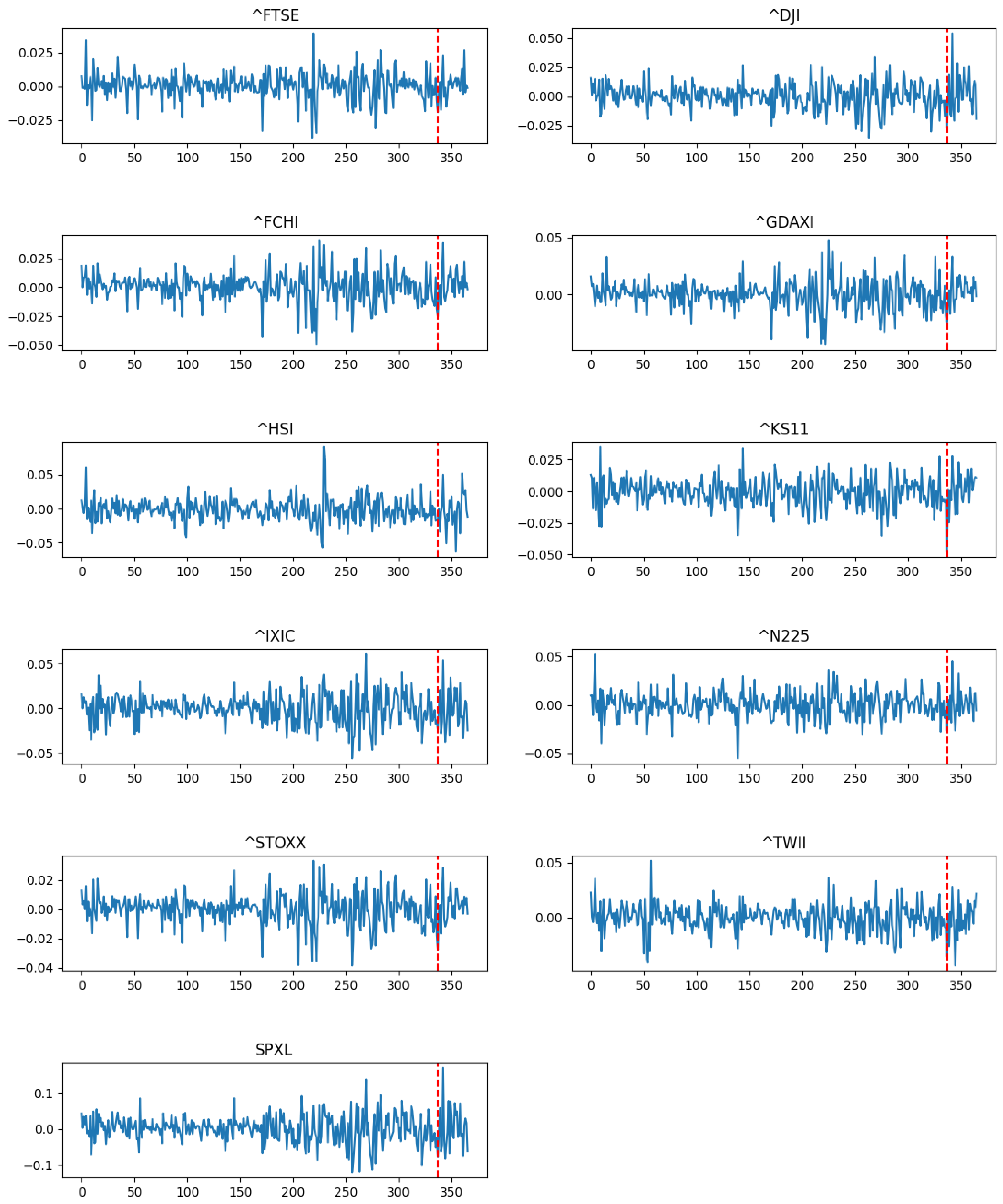
Here, we use the daily stock close index data of FTSE, DJI, FCHI, GDAXI, HSI, KS11, IXIC, N225, ST0XX, TWII, and SPXL from 2 February 2021 to 9 November 2022 as the raw data and let 23 September 2022 be the intervention date when the mini-budget was delivered as a ministerial statement by the then Chancellor of the Exchequer, Kwasi Kwarteng. All the stock market datasets are collected from Yahoo Finance using the Python package “yfinance”. The stock price indexes are shown in Figure 1, where the red vertical line represents the intervention time. We observe from this figure that most of the series are non-stationary. To make these series stationary, we transfer the daily stock price data into daily return data through $r_t=(P_t-P_{t-1})/P_{t-1}$, where $P_t$ and $P_{t-1}$ are the daily closing prices of the index on day t and $t-1$, respectively. The time series of the daily return data all look stationary as shown in Figure 2.

Since the stock trading is not done everyday, we regard 26 September 2022, which is the first observable time point immediately following the intervention, as the first post-intervention time point. Following the no anticipation contextual requirement by Abadie [14], the synthetic control estimators may be biased if forward-looking economic agents react in advance of the policy intervention, while backdating the intervention in the data does not mechanically bias the estimator of the effect. Therefore, we backdate the intervention to 5 September 2022 before Truss became prime minister when little of the anticipation effect can be expected. Additionally, on the one hand, since the stock trading dates are slightly different in various countries, we take the intersection of the trading dates of all the 11 stock indexes to unify the trading dates for them. Then, based on the unified data, we can apply the synthetic control method to estimate the potential outcomes and thus the causal effects. On the other hand, the trading dates are not consecutive, which may lead to some problem while plotting the series, so we transfer the dates into consecutive integers according to the date index (e.g., 20210202 with date index 0 and 20210203 with date index 1, etc.) so that we obtain date consecutive stock index series.

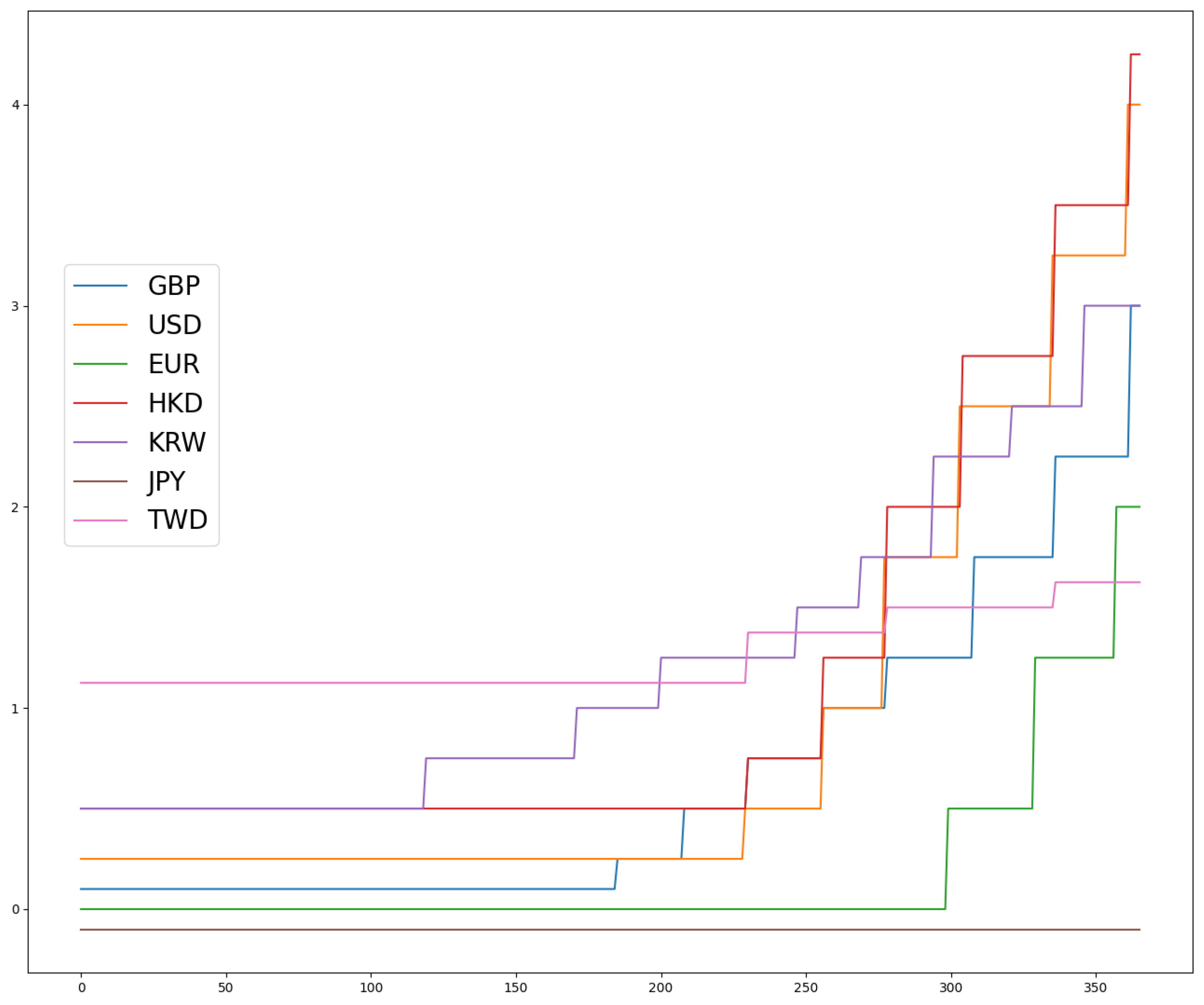
In addition to the stock index daily return as the outcome, we also consider the interest rate as the covariate while implementing the synthetic control method because among the financial factors, changes in the interest rate level have very direct and rapid impact on the stock market. Generally, when interest rates fall, stock prices rise; when interest rates rise, stock prices fall. Moreover, due to the epidemic of COVID-19, a lot of governments around the world have adopted quantitative easing policies to stimulate the economy, which may lead to inflation. Therefore, after the epidemic stabilised, in order to avoid hyperinflation, central banks started raising the interest rates to control inflation. And the drastic rate hike policies must have significant influence on the stock market. Therefore, in addition to daily return, we take the interest rate data of transaction currency for the 11 indexes as the covariate in synthetic control method. This means that we hope to obtain a synthetic unit whose stock index and corresponding interest rate are close to the properties for the FTSE. We will compare it with the observed FTSE series to estimate the causal effect. The series of interest rates for the corresponding transaction currencies are shown in Figure 3. After processing and summarising the data, we will apply the synthetic control method, the modified synthetic control and synthetic difference in difference (SDID) method, respectively, to evaluate the causal effect of mini-budget policy and compare their performances.

4.2. Evaluating the Causal Effect of the Mini-Budget by Conventional Synthetic Control

In this subsection, we tend to estimate the causal effect of the mini-budget through the conventional synthetic control method. In order to evaluate the performance of this method, we need to set a metric that could reflect the performance of the model. Moraffah et al., 2021 [15] summarised some evaluation metrics, which can be used to measure the performance of a causal model in terms of causal discovery power or causal effect inference power and three of the proposed metrics (mean squared error (MSE), F-test, and T-test) are suitable to evaluate the performance of causal effect inference models; that is of interest to us. Moreover, Abadie 2021 [14] suggests the root mean squared prediction error (RMSPE) as the evaluation metric for synthetic control method which is equivalent to the pre-intervention MSE. Therefore, in this empirical study, we select MSE as the metric to evaluate the performance of the causal inference methods, which compares the estimated potential outcome series with the pre-intervention ground truth series by taking the average of the squared differences at each pre-intervention time.

By applying conventional synthetic control method, which balances both the stock index daily return and the corresponding interest rate, we could obtain the synthetic weights and estimate the potential daily returns of FTSE in the absence of the effect of mini-budget policy after its implementation time. Based on the synthetic control result, only FCHI and STOXX are selected from the 10 control indexes to synthesise FTSE with estimated synthetic weights 0.6534 and 0.3465, respectively. In detail, the potential outcomes of FTSE after intervention could be estimated by:

$${\widehat{FTSE}}_t=0.653443\ast FCH{I}_t+0.346471\ast STOX{X}_t\mathrm{for}t>T_0$$

(18)

with the synthetic weights determined by:

$$\underset{\begin{array}{c}{w}_2,\dots ,w_{J+1}\ge 0,\\ {\displaystyle \sum _{j=2}^{J+1}}{w}_j=1\end{array}}{argmin}\sum _{t=1}^{T_0}\left\{{(Y_{1t}-\sum _{j=2}^{J+1}{\omega }_j{Y}_{jt})}^2+{(r_{1t}-\sum _{j=2}^{J+1}{\omega }_j{r}_{jt})}^2\right\},$$

(19)

where $Y_{1t}$ represents the daily return of FTSE, while $Y_{jt}$ for $j\ge 2$ represents the daily returns of other stock indexes except FTSE, and $r_{jt}$ denotes the corresponding interest rate of the currency used by stock index j at time t. When $j=1$, $r_{1t}$ represents the interest rate of the currency used by FTSE, which is GBP.

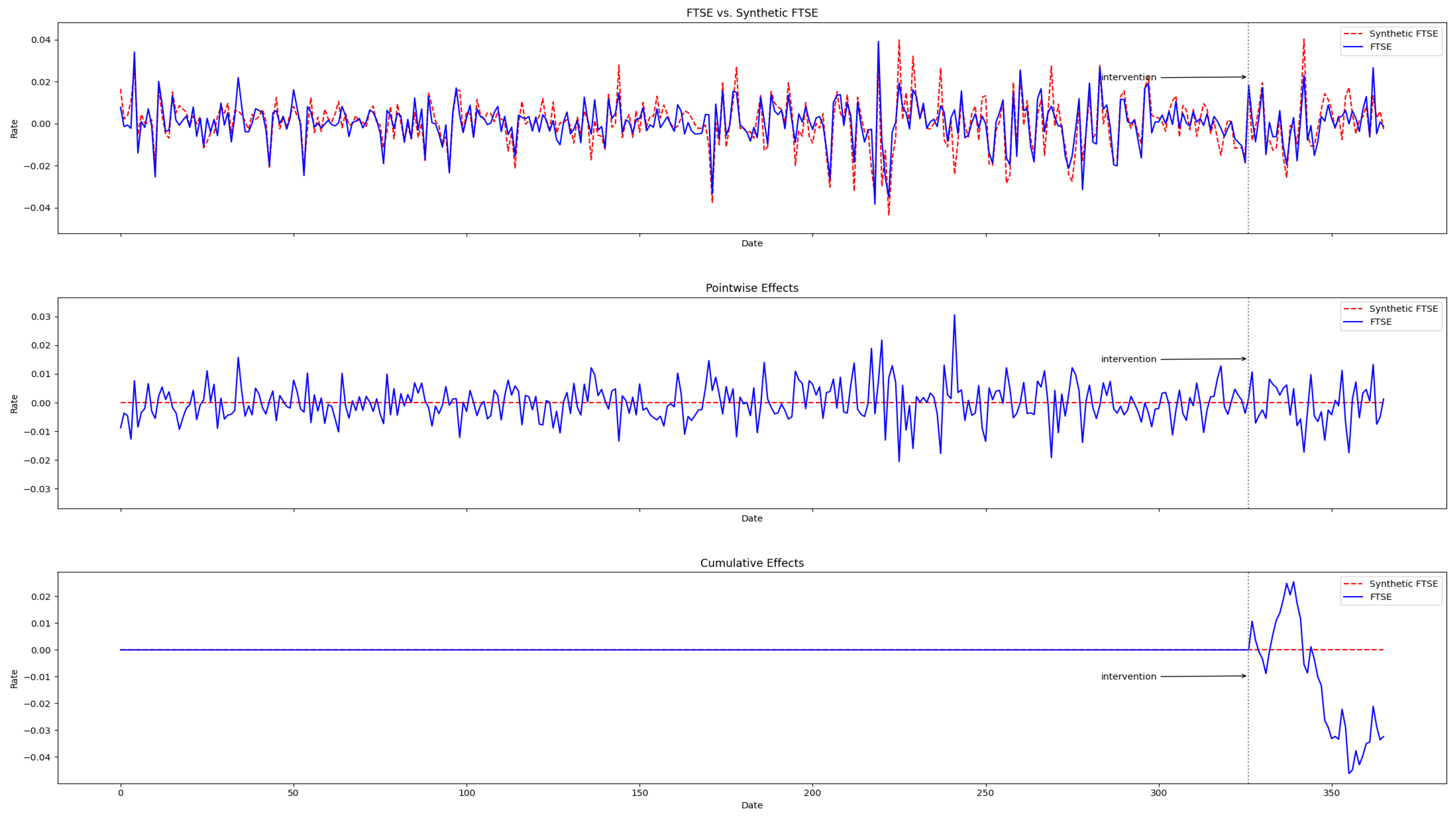
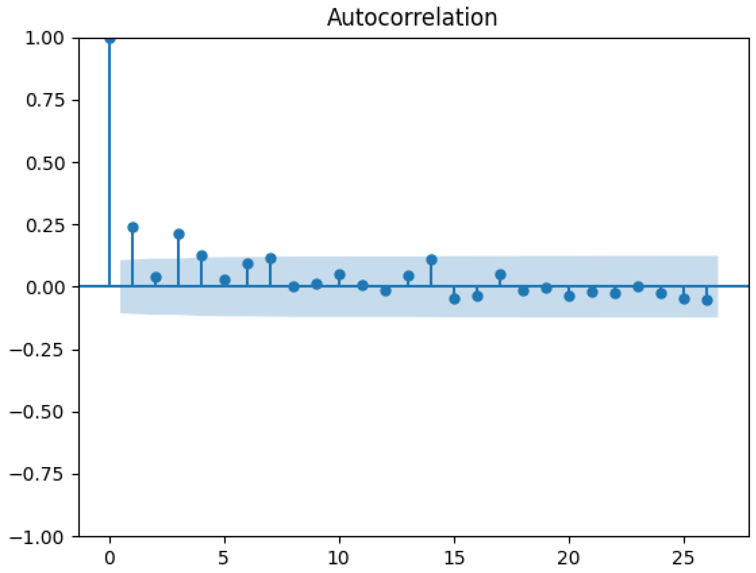
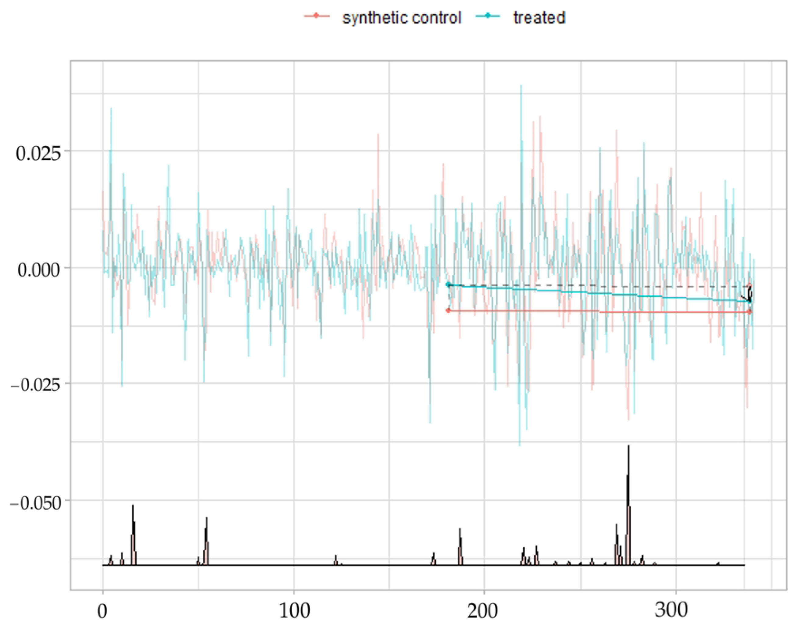
As the synthetic result shown in Figure 4, we could observe that the pre-intervention fitness of the conventional synthetic control method is fairly good. Especially in terms of the growing or declining trend, the synthetic series could follow the true series closely. However, it is obvious that the volatility of the synthetic series is usually higher than that of the real series, with higher peaks and lower valleys. This implies the conventional synthetic control method cannot accurately capture the fluctuation property of the true series. Moreover, in terms of the middle panel in Figure 4, the scale of the residuals across time is not stable, which implies there exists heteroskedasticity in the residual series and this may affect our inference on the causal effect. In terms of the performance of the synthetic control method, the MSE of daily return is 0.40561, with the number of pre-intervention period $T_0=327$. In addition to the MSE, we also test the autocorrelation of both the squared true FTSE daily returns and the squared synthetic FTSE daily returns. As shown in Figure 5 and Figure 6 we could observe that the autocorrelation characteristics of the squared true FTSE daily return series, which has first- and third-order autocorrelations, and the squared synthetic FTSE daily return series by the conventional synthetic control method are significantly different. This phenomenon can further support our conjecture that the synthetic series produced by the conventional synthetic control method is not able to cover the heteroskedasticity of the original series.

Considering the causal effect of the mini-budget, we select the period between 26 September 2022 and 4 November 2022, which contains the next 30 trading days after the intervention, as the affected period and regard the accumulated causal effect during this period as the metric to evaluate the effect caused by the mini-budget policy. The result by the conventional synthetic control method illustrates that the accumulated effect of the mini-budget policy on FTSE return is ${\widehat{\tau }}^{cum}=-0.04607$ in the next 30 trading days. This is the accumulated causal effect on the daily return, while when transferred to index data, the effect will be more significant. And we will show the potential index after intervention through conventional and modified synthetic control methods and compare them in the next subsection.

4.3. Evaluating the Causal Effect of Mini-Budget by the Modified Synthetic Control

After applying the conventional synthetic control method in the last subsection, we notice that the heteroskedasticity of the series is not considered by the conventional method, which may affect the quality of the synthetic potential outcomes. Therefore, in this section, we use the modified synthetic control method to overcome this problem. Compared to the conventional synthetic control method, the modified synthetic control method additonally considers the absolute value of the outcome as a covariate while determining the synthetic weights. By the modified synthetic control method, we obtain different synthetic weights from the conventional synthetic control method. The result illustrates that, different from the conventional method, STOXX and N225 are chosen from the donor pool, which contains all the control units, with synthetic weights 0.873342 and 0.126635, respectively. In detail, the potential outcomes of FTSE after intervention are estimated by:

$${\widehat{FTSE}}_t=0.873342\ast STOX{X}_t+0.126635\ast N{225}_t\mathrm{for}t>T_0$$

(20)

with the synthetic weights determined by:

$$\underset{\begin{array}{c}{w}_2,\dots ,w_{J+1}\ge 0,\\ {\displaystyle \sum _{j=2}^{J+1}}{w}_j=1\end{array}}{argmin}\sum _{t=1}^{T_0}\left\{{(Y_{1t}-\sum _{j=2}^{J+1}{\omega }_j{Y}_{jt})}^2+(|Y_{1t}{|-\sum _{j=2}^{J+1}{\omega }_j\left|Y_{jt}\right|)}^2+{(r_{1t}-\sum _{j=2}^{J+1}{\omega }_j{r}_{jt})}^2\right\},$$

(21)

where $Y_{it}$ also represents the daily return of stock index i at time t and $r_{jt}$ denotes the corresponding interest rate of the currency used by stock index j at time t. Corresponding to Equation (10), the choice of $v_i$’s in this real data analysis are just taken as 1 for simplicity, and there seems to be no particular prior information telling us which equation in (9) should be more considered.

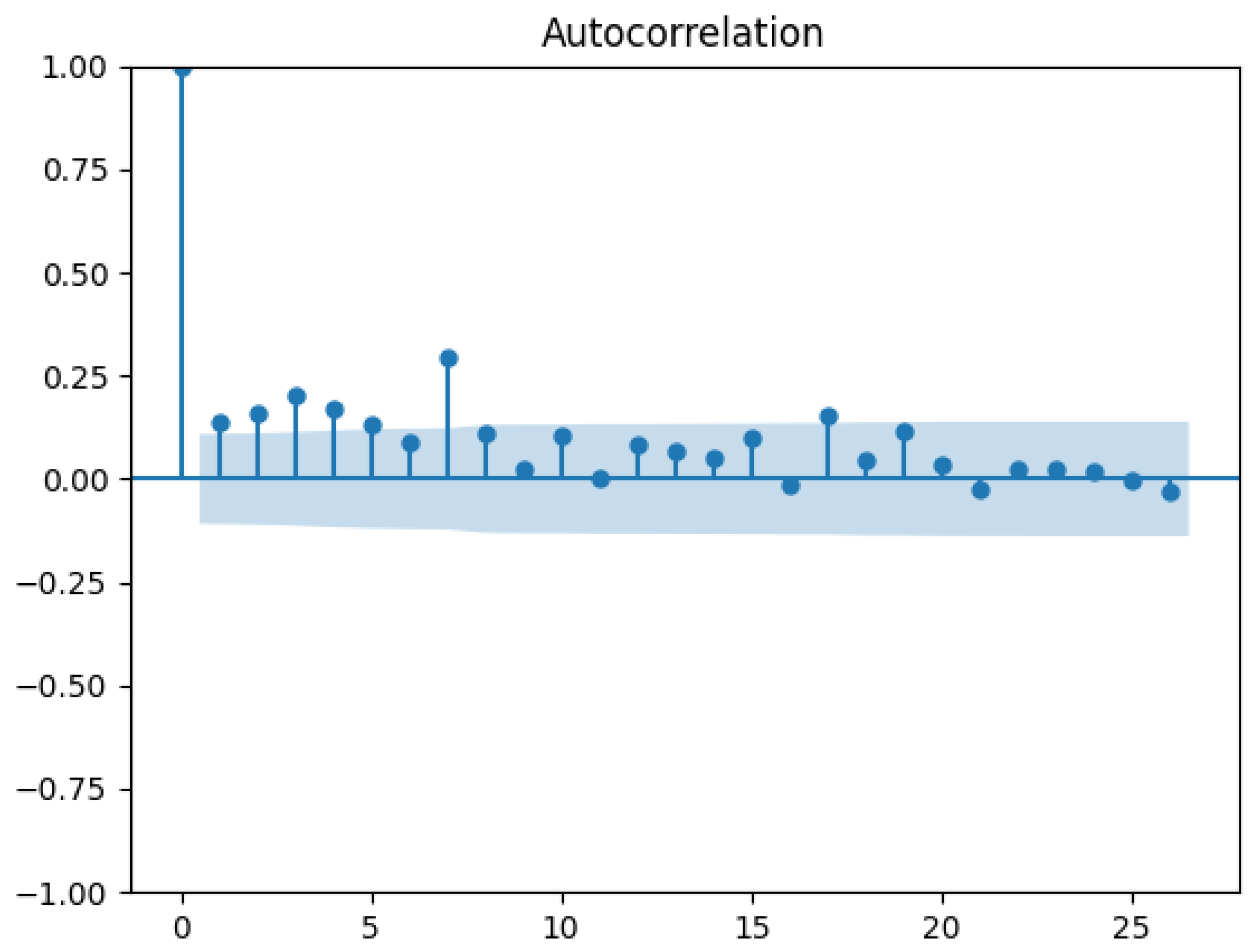
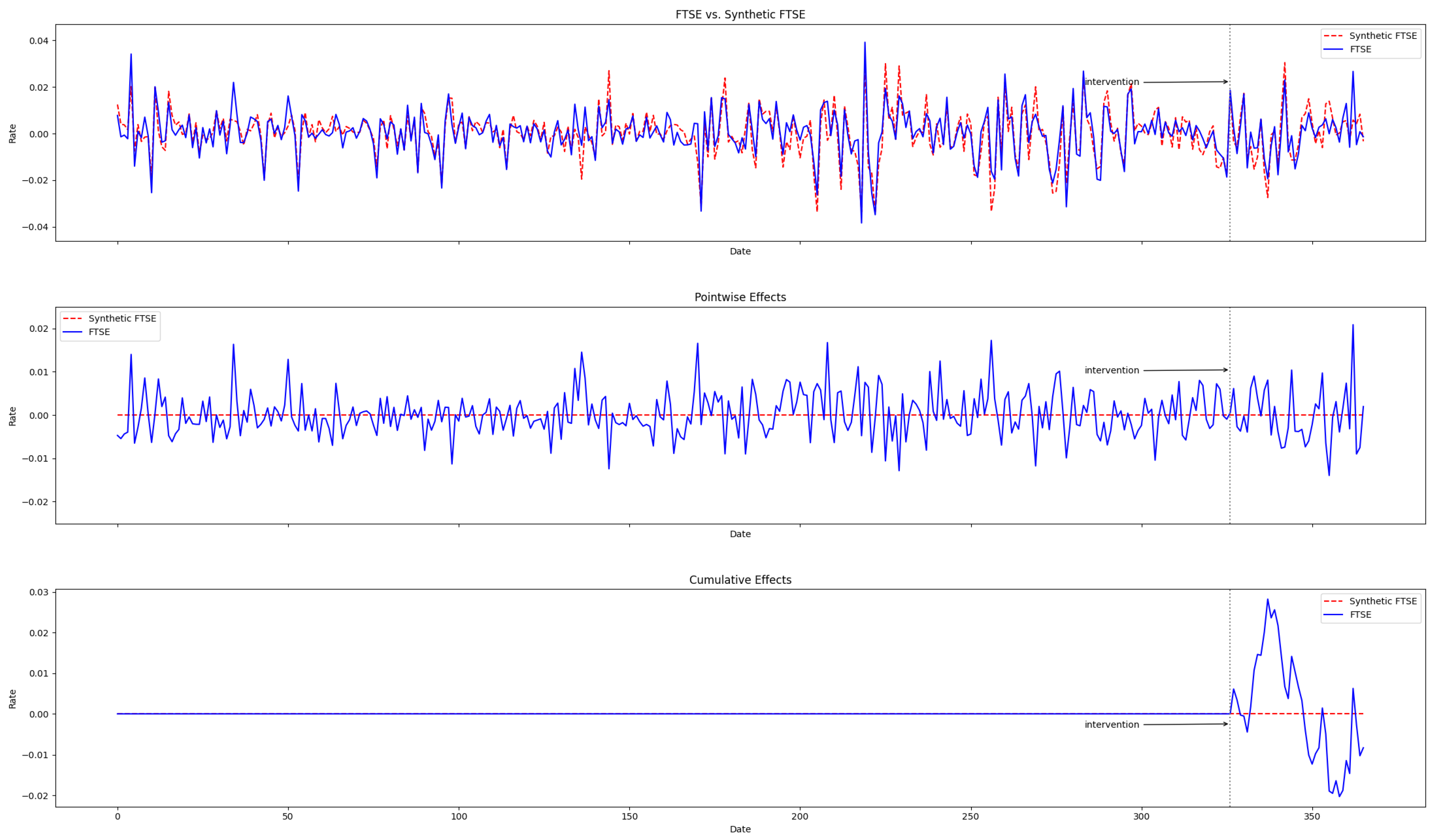
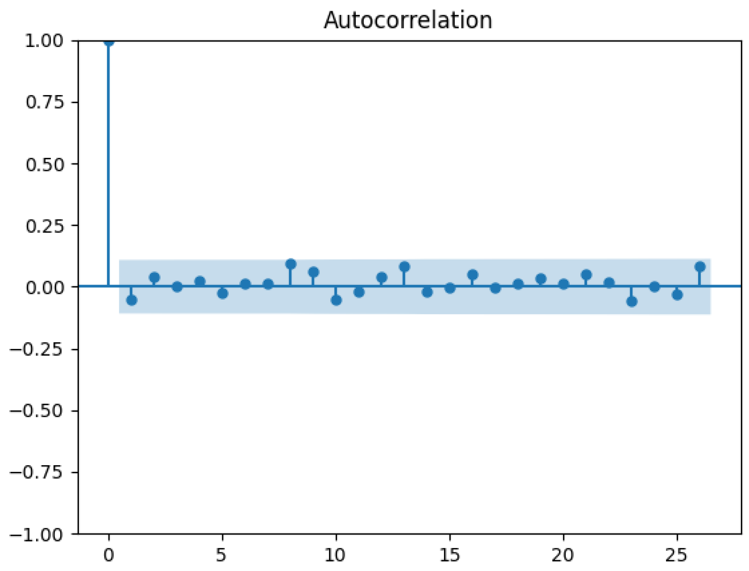
By comparing the modified synthetic result in Figure 7 to the conventional synthetic result in Figure 4, we can see in the top panel that the synthetic FTSE series fits the true FTSE series better than the result by conventional synthetic control during the pre-intervention period, especially at the peaks and valleys of the series. This implies that the fluctuation of the synthetic series is well controlled to be more similar to the fluctuation of the true FTSE series by the modified synthetic control method. And we tend to attribute this progress to the introduction of the absolute return, which could help control the volatility of the synthetic series. In terms of the second panel above, we can observe that the fluctuation scale of pre-intervention fitting error series is much more stable than the pre-intervention error series produced by conventional synthetic control, which implies that the error series is essentially homoskedastic. This means that the conditional heteroskedasticity of the original series is covered by the modified synthetic control method. In order to further demonstrate the advantage of the modified synthetic control method in terms of its ability to cover the conditional heteroskedasticity, we also test the autocorrelation of squared residuals by the conventional synthetic control method and the modified synthetic control method shown in Figure 8 and Figure 9, respectively.

According to the two autocorrelograms, we could easily observe that the residual series by modified synthetic control outperforms the residual series by the conventional synthetic control method since there is no significant autocorrelation of the squared residual series by modified synthetic control while for the conventional synthetic control, the autocorrelation of its squared residual series is relatively more significant. This means that the left heteroskedasticity in the residual series is not expressed by the conventional method and might lead to worse inference of the causal effect. Interestingly, our modified synthetic control generates less informative residuals (i.e., more like a purely white noise) than the residuals from the conventional synthetic control, as indicated in Figure 8 and Figure 9. In this sense, our modified synthetic control is preferred.

Moreover, turning to the goodness of fit of and causal inference result by the modified synthetic control model, the MSE of daily return is 0.2480, which is reduced by $40\%$ compared to the MSE of the conventional synthetic control method with $MSE=0.4056$. This implies that the introduction of absolute return in the modified synthetic control method could significantly improve the pre-treatment fit of the conventional synthetic control method at least in this empirical study. In terms of the estimated causal effect of the mini-budget by this modified method, as we do for the conventional synthetic control method, we still select the period between 26 September 2022 and 4 November 2022, which contains the next 30 trading days after the intervention, as the affected period and regard the accumulated causal effect during this period as a metric to evaluate the causal effect. According to the comparison between observed outcomes of FTSE and synthetic outcomes by the modified synthetic control method, we conclude that the causal effect of the mini-budget on the FTSE index return is ${\widehat{\tau }}^{cum}=-0.0220$, which is less than half of the estimation result by the conventional synthetic control method. And based on the performances of both of these synthetic control methods, we tend to conclude that the conventional synthetic control method significantly overestimates the scale of the causal effect by the mini-budget policy compared to the modified synthetic control method, which has both lower MSE and better homoskedastic properties.

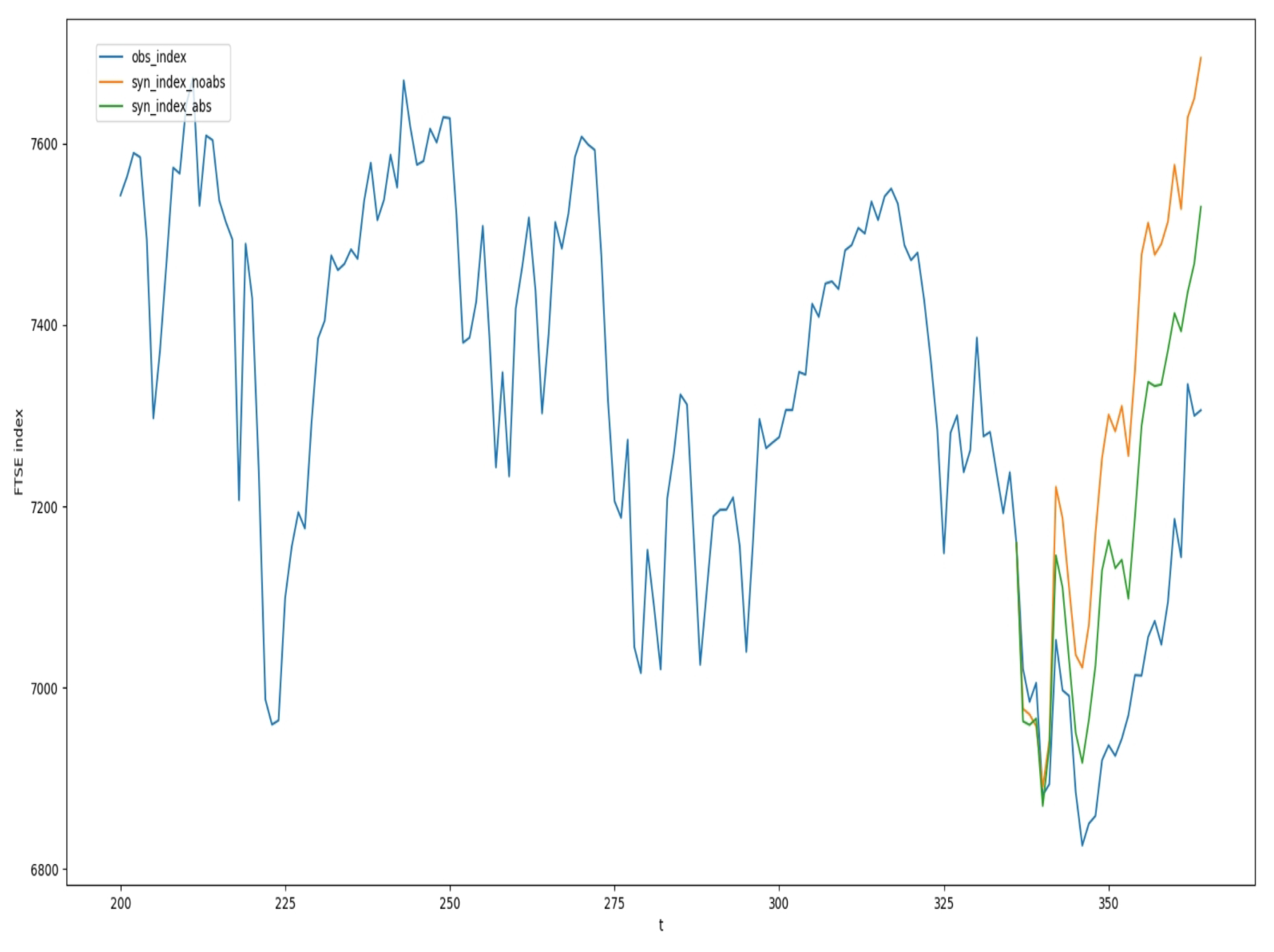
To demonstrate the difference between the two synthetic control methods more clearly, we transfer the daily return data back into stock index daily close price data. Since the intervention was taken on 23 September 2022, we let the last trading day before intervention (22 September 2022) be the starting point and calculate the estimated synthetic index through multiplying $(1+r)$ with the last day’s close index where r is the synthetic daily return. The comparison among the true FTSE index series and two synthetic series are shown in Figure 10.

As shown in the figure, it is obvious that after promulgating the mini-budget policy, there is a sharp decrease in the FTSE index, which is likely to be caused by the mini-budget to a large extent, while also by other factors to some mild extend. Our target in the causal effect inference is to precisely estimate the effect of the intervention of our interest while eliminating the effect of other factors. Thus, the question here is how much of the change comes from the mini-budget intervention. Therefore, we apply conventional and modified synthetic control methods to construct the potential outcome series of FTSE which are shown by the yellow line and green line, respectively. In the next 5 trading days after intervention, 337–341 (26 September 2022 to 5 October 2022), the three indexes experience similar decrease trends. However, they begin to show significant difference from their rebounding at 342, where the two synthetic FTSE series have more substantial growth while the real FTSE just rises a little. After the rising trend, although the three series all experience similar downtrends until 346 (10 December 2022), the divergence among the three series still stays almost stable. After 346, even if all the three series grow rapidly, the differences among them become larger because of different growth rates. Considering the previous conclusion of the two synthetic control models, the green line generated by modified SC model should be the best estimation of the potential outcomes in terms of both the perspective of pre-treatment fit and its ability to control heteroskedasticity of residual series. Therefore, we reasonably think that the conventional synthetic control model seriously overrates the potential outcomes of the FTSE index after intervention and thus overestimates the scale of the causal effect caused by the mini-budget policy on the UK stock market. And the milder causal effect estimation given by the modified synthetic control is considered to be more reasonable.

4.4. Evaluating the Causal Effect of the Mini-Budget by Synthetic Difference in Difference

In addition to the comparison between the two synthetic control methods, we also tend to compare them with synthetic difference in difference method (SDID) in this subsection to see their performance in average causal effect inference. Synthetic DID is a causal inference method proposed by Arkhangelsky et al., 2021 [16], which combines the ideas of both synthetic control and difference in differences. It does not require one to synthesise a series to fit the observed treated series very well by the control series like the synthetic control method while the synthetic DID tends to synthesise a series parallel to the observed treated series. In other words, it can accept a fixed intercept in the linear synthetic, and then apply the difference in difference (DID) method (see Bowers et al. [17]; Abadie [18]; Callaway et al. [19]; Card et al. [20]; Bertrand et al. [21]) on the parallelised series to eliminate the effect of confounding factors while estimating the causal effect. Moreover, different from the conventional synthetic control which gives a potential outcome series after intervention by weighted averaging the control unit series, synthetic DID additionally weights the outcomes along the time and gives an integrated result as an estimation of the average treatment effect. However, although learning good properties of synthetic control and DID, the synthetic DID omits an important property from synthetic control, that SDID does not consider covariates while determining the weights. The target of the synthetic control method is not only to generate an outcome series which matches the observed series very well but one that also requires the covariates of the synthetic unit match the observed treated unit’s covariates well, through which we can obtain a similar unit to the observed treated unit in terms of every aspect except for the treatment assignment; thus, the influence of the confounding factors could be effectively eliminated. However, SDID only considers the outcome series and does not care about the covariates, which means that although SDID uses a synthetic framework similar to synthetic control, the basic idea of SDID is not essentially the same as the idea of synthetic control. SDID does not try to eliminate the influence of confounding factors through constructing a perfect unit with outcomes and covariates similar to the treated unit like the synthetic control method does; it instead makes use of the idea of DID to eliminate the confounding factors after the parallel assumption is well prepared by the synthetic idea.

The integrated result by SDID represents the fixed causal effect of intervention on the treated unit at any time t for $t>T_0$. Therefore, the result can be compared with the average causal effect $\widehat{\overline{\tau }}$ estimated by the two synthetic control methods. The causal effect series for a long time after the intervention is not stationary as shown by the previous synthetic control method results, which means the causal effects along the time may not have the same expectation. Therefore, the mean value for such a non-stationary series without identical expectation is not sufficient to be a metric to evaluate the causal effect. Thus, we tend to select a relative short period after intervention, during which the expectation of the causal effects at different times are similar to each other, then the average causal effect could be regarded as a reasonable metric to evaluate the causal effect of the mini-budget. So the average causal effect in the next five trading days after intervention is considered as a metric to evaluate the average causal effect of the mini-budget policy. We apply SDID on the FTSE daily return series ending at 341 (30 September 2022) by using the R (Version 4.2.1) package “synthdid” to estimate the average causal effect of the mini-budget. By limiting the time period before 341 we can calculate the conditional mean treatment effect in the next five trading days after the intervention using SDID, the conventional synthetic control method and the modified synthetic control method. The synthetic result by SDID is shown in Figure 11 and the synthetic weights including period weights and unit weights are shown in

Table 1. The period weights and unit weights of the SDID.

Unit Weights		Period Weights
Name	Weight	Time	Weight
FCHI	0.124	4	0.020
STOXX	0.126	10	0.027
GDAXI	0.121	16	0.127
KS11	0.103	50	0.018
DJI	0.107	54	0.100
TWII	0.101	122	0.022
N225	0.102	173	0.027
HSI	0.099	187	0.078
IXIC	0.078	220	0.037
		223	0.017
		227	0.041
		269	0.087
		271	0.040
		275	0.253
		282	0.020

. In terms of the result produced by SDID, the estimated average treatment effect of the mini-budget is ${\widehat{\tau }}_{SDID}=-0.00329$. And we tend to take the standard error of the estimators, like Arkhangelsky et al. [16] did, as a metric to evaluate them so that the results from different methods could be compared reasonably. The estimation results and standard errors of the average treatment effects based on these three methods are demonstrated in

Table 2. Average causal effect estimation by the 3 methods.

	Conventional SC	Modified SC	SDID
Average causal effect	−0.00608	−0.00431	−0.00329
Stand error	0.00317	0.00156	0.00175

. We could see that the modified synthetic control method outperforms the other two methods in terms of the standard error. In causal inference problems, less standard error usually implies that more confounding factors are considered; thus, the estimation result of causal effect is more stable and reliable. On the one hand, compared to the conventional synthetic control method, the modified synthetic control decreases the standard error of the conventional synthetic control method by about 50%, which implies that in estimating the average causal effect, the modified synthetic control method still outperforms the conventional synthetic control method significantly. On the other hand, in terms of the comparison between the modified synthetic control method and SDID, their standard errors are similar to each other and the modified synthetic control method even slightly outperforms SDID, which is especially designed for average causal effect inference. This might imply that when the suitable covariates are selected, the modified synthetic control method could also have a very good performance in estimating the average causal effect while the performance of conventional synthetic control is not desirable enough.

5. Conclusions

This study proposed a modified synthetic control method which can improve the causal inference ability of the conventional synthetic control method. Compared to the conventional synthetic control method, the modified method additionally considers the absolute value of the outcomes to control the volatility of the synthetic series, which can effectively improve the performance of the conventional synthetic control. Motivated by the heteroskedasticity of the time series, widely found in financial time series data but not considered by the conventional synthetic control method, we propose the modified synthetic control method to bridge this gap and introduce its framework and the synthetic weight determination process with the theoretical consistency of the synthetic weights determined by it established.

By the proposed method, we carry out an empirical study in evaluating the causal effect of the mini-budget policy on the UK stock market to test the performance of the modified synthetic control method. According to the empirical study result, the modified synthetic control method significantly outperforms the conventional synthetic control in terms of not only the pre-treatment fitness, illustrated by the pre-treatment MSE, but also covering the heteroskedasticity of the pre-treatment residual series. The autocorrelation result demonstrates that there exists no autocorrelation of the squared pre-treatment residual series by the modified synthetic control method, while the squared pre-treatment residual series by the conventional synthetic control method is still obviously autocorrelated. This implies that the conditional heteroskedasticity of the true pre-treatment series, which is not covered by the conventional synthetic control method, has been reasonably characterised by the modified synthetic control method. These two aspects of progress reflect the superiority of the modified synthetic control method.

In addition, we also apply the synthetic difference in difference method in the empirical study as a comparison with the modified synthetic control method to show its ability in estimating the average treatment effect. The empirical study result illustrates that the modified synthetic control method performs best among the three methods, at least in this empirical study under reasonable settings. This means that if we could select relatively reasonable covariates, the modified synthetic control method could even perform better than SDID in the average causal effect estimation, which is specifically designed for average treatment effect estimation while the conventional synthetic control method is not. This result further demonstrates the advantage of the modified synthetic control method especially while comparing to the conventional synthetic control method and also shows its potential ability in estimating the average causal effect.

References

1. Abadie, A.; Diamond, A.; Hainmueller, J. Synthetic control methods for comparative case studies: Estimating the effect of California’s tobacco control program. J. Am. Stat. Assoc. 2010, 105, 493–505. [Google Scholar] [CrossRef]
2. Künzel, S.R.; Sekhon, J.S.; Bickel, P.J.; Yu, B. Metalearners for estimating heterogeneous treatment effects using machine learning. Proc. Natl. Acad. Sci. USA 2019, 116, 4156–4165. [Google Scholar] [CrossRef] [PubMed]
3. Wager, S.; Athey, S. Estimation and inference of heterogeneous treatment effects using random forests. J. Am. Stat. Assoc. 2018, 113, 1228–1242. [Google Scholar] [CrossRef]
4. Esposti, M.D.; Spreckelsen, T.; Gasparrini, A.; Wiebe, D.J.; Bonander, C.; Yakubovich, A.R.; Humphreys, D.K. Can synthetic controls improve causal inference in interrupted time series evaluations of public health interventions? Int. J. Epidemiol. 2020, 49, 2010–2020. [Google Scholar] [CrossRef]
5. Chernozhukov, V.; Wüthrich, K.; Zhu, Y. An exact and robust conformal inference method for counterfactual and synthetic controls. J. Am. Stat. Assoc. 2021, 116, 1849–1864. [Google Scholar] [CrossRef]
6. Athey, S.; Imbens, G.W. The state of applied econometrics: Causality and policy evaluation. J. Econ. Perspect. 2017, 31, 3–32. [Google Scholar] [CrossRef]
7. Splawa-Neyman, J.; Dabrowska, D.M.; Speed, T.P. On the Application of Probability Theory to Agricultural Experiments. Essay on Principles. Section 9. Statist. Sci. 1990, 5, 465–472. [Google Scholar] [CrossRef]
8. Rubin, D.B. Estimating causal effects of treatments in randomized and nonrandomized studies. J. Educ. Psychol. 1974, 66, 688. [Google Scholar] [CrossRef]
9. Rubin, D.B. Causal inference using potential outcomes: Design, modeling, decisions. J. Am. Stat. Assoc. 2005, 100, 322–331. [Google Scholar] [CrossRef]
10. Rosenbaum, P.R.; Rubin, D.B. The central role of the propensity score in observational studies for causal effects. Biometrika 1983, 70, 41–55. [Google Scholar] [CrossRef]
11. Ben-Michael, E.; Feller, A.; Rothstein, J. The augmented synthetic control method. J. Am. Stat. Assoc. 2021, 116, 1789–1803. [Google Scholar] [CrossRef]
12. Mandelbrot, B.B. The Variation of Certain Speculative Prices. J. Bus. 1963, 36, 394–419. [Google Scholar] [CrossRef]
13. Granger, C.W.J.; Ding, Z. Some Properties of Absolute Return: An Alternative Measure of Risk. Ann. Econ. Stat. 1995, 67–91. [Google Scholar] [CrossRef]
14. Abadie, A. Using synthetic controls: Feasibility, data requirements, and methodological aspects. J. Econ. Lit. 2021, 59, 391–425. [Google Scholar] [CrossRef]
15. Moraffah, R.; Sheth, P.; Karami, M.; Bhattacharya, A.; Wang, Q.; Tahir, A.; Raglin, A.; Liu, H. Causal inference for time series analysis: Problems, methods and evaluation. Knowl. Inf. Syst. 2021, 63, 3041–3085. [Google Scholar] [CrossRef]
16. Arkhangelsky, D.; Athey, S.; Hirshberg, D.A.; Imbens, G.W.; Wager, S. Synthetic difference in differences. Am. Econ. Rev. 2021, 111, 4088–4118. [Google Scholar] [CrossRef]
17. Bowers, J.; Fredrickson, M.M.; Panagopoulos, C. Reasoning about interference between units: A general framework. Political Anal. 2013, 21, 97–124. [Google Scholar] [CrossRef]
18. Abadie, A. Semiparametric difference in differences estimators. Rev. Econ. Stud. 2005, 72, 1–19. [Google Scholar] [CrossRef]
19. Callaway, B.; Sant’Anna, P.H.C. Difference-in-differences with multiple time periods. J. Econom. 2021, 225, 200–230. [Google Scholar] [CrossRef]
20. Card, D.; Krueger, A.B. Minimum Wages and Employment: A Case Study of the Fast Food Industry in New Jersey and Pennsylvania. Am. Econ. Rev. 1994, 84, 772–793. [Google Scholar]
21. Bertrand, M.; Duflo, E.; Mullainathan, S. How much should we trust differences-in-differences estimates? Q. J. Econ. 2004, 119, 249–275. [Google Scholar] [CrossRef]
22. Merlevede, F.; Peligrad, M.; Rio, E. Bernstein inequality and moderate deviations under strong mixing conditions. In High Dimensional Probability V: The Luminy Volume; Institute of Mathematical Statistics: Beachwood, OH, USA, 2009; Volume 5, pp. 273–292. [Google Scholar]
Figure 1. The stock price indexes, with the red vertical line representing the intervention time.
Mathematics 12 03301 g001
Figure 2. The stock index daily return series, where the red vertical lines represent the intervention time.
Mathematics 12 03301 g002
Figure 3. Interest rate series of the 7 currencies.
Mathematics 12 03301 g003
Figure 4. Conventional synthetic result. Top panel: FTSE return shown by the solid blue line and conventional synthetic FTSE shown by the red dotted line. Middle panel: the blue solid line after intervention represents the estimated individual treatment effects for each date. The red dotted line illustrates the treatment effect on the conventional synthesised potential outcome which is obviously always 0. Bottom panel: The blue line after intervention represents the cumulative effect for the treated unit until certain dates.
Mathematics 12 03301 g004
Figure 5. Autocorrelation of the squared FTSE daily return series.
Mathematics 12 03301 g005
Figure 6. Autocorrelation of the squared daily return series by conventional synthetic control ( F T S E ^ t = 0.653443 F C H I t + 0.346471 S T O X X t ).
Mathematics 12 03301 g006
Figure 7. Modified synthetic result. Top panel: FTSE return shown by the solid blue line and modified synthetic FTSE shown by the red dotted line. Middle panel: the blue solid line after intervention represents the estimated individual treatment effects for each date. The red dotted line illustrates the treatment effect on the modified synthesised potential outcome which is obviously always 0. Bottom panel: The blue line after intervention represents the cumulative effect for the treated unit until certain dates.
Mathematics 12 03301 g007
Figure 8. Autocorrelation of the squared residuals by the conventional synthetic control method ( F T S E ^ t = 0.653443 F C H I t + 0.346471 S T O X X t ).
Mathematics 12 03301 g008
Figure 9. Autocorrelation of squared residuals by modified synthetic control method ( F T S E ^ t = 0.873342 S T O X X t + 0.126635 N 225 t ).
Mathematics 12 03301 g009
Figure 10. Comparison of the synthetic series and observed FTSE series.
Mathematics 12 03301 g010
Figure 11. The synthetic control DID result.
Mathematics 12 03301 g011