Article

Variational Bayesian EM Algorithm for Quantile Regression in Linear Mixed Effects Models

1
School of statistics and Mathematics, Central University of Finance and Economics, Beijing 102206, China
2
Department of Medical Engineering and Technology, Xinjiang Medical University, Urumqi 830011, China
*
Author to whom correspondence should be addressed.
Mathematics 2024, 12(21), 3311; https://doi.org/10.3390/math12213311
Submission received: 11 September 2024 / Revised: 2 October 2024 / Accepted: 21 October 2024 / Published: 22 October 2024
(This article belongs to the Section Probability and Statistics)

Abstract

:
This paper extends the normal-beta prime (NBP) prior to Bayesian quantile regression in linear mixed effects models and conducts Bayesian variable selection for the fixed effects of the model. The choice of hyperparameters in the NBP prior is crucial, and we employed the Variational Bayesian Expectation–Maximization (VBEM) for model estimation and variable selection. The Gibbs sampling algorithm is a commonly used Bayesian method, and it can also be combined with the EM algorithm, denoted as GBEM. The results from our simulation and real data analysis demonstrate that both the VBEM and GBEM algorithms provide robust estimates for the hyperparameters in the NBP prior, reflecting the sparsity level of the true model. The VBEM and GBEM algorithms exhibit comparable accuracy and can effectively select important explanatory variables. The VBEM algorithm stands out in terms of computational efficiency, significantly reducing the time and resource consumption in the Bayesian analysis of high-dimensional, longitudinal data.

1. Introduction

Regression modeling for high-dimensional data has become increasingly prevalent in modern statistical applications. In such scenarios, the number of covariates, denoted as p , often far exceeds the number of observations, denoted as n . Many of these covariates are typically irrelevant, and the inclusion of numerous covariates may adversely affect parameter estimation, leading to what is known as the “curse of dimensionality” [1]. Therefore, variable selection is crucial in modeling high-dimensional data. Current variable selection methods can be broadly categorized into two classes. The first class comprises penalty likelihood methods, including classical techniques such as Akaike Information Criterion (AIC), Bayesian Information Criterion (BIC), Least Absolute Shrinkage and Selection Operator (LASSO), and Smoothly Clipped Absolute Deviation (SCAD). These methods minimize the penalized function of the logarithmic likelihood and regression coefficients. By selecting an appropriate penalty function, certain components of regression coefficients are forced to be zero, achieving simultaneous parameter estimation and variable selection. The second class involves Bayesian methods, which assign a hierarchical prior to all unknown parameters. Bayesian inference is then conducted by combining the prior on unknown parameters with the model likelihood, yielding posterior distributions for the parameters. A notable advantage of Bayesian methods is the ability to obtain posterior distributions for all submodels. Additionally, in terms of prediction, model combinations often outperform individual models. Consequently, Bayesian variable selection methods are advantageous.
Mixed effects models are employed for modeling and analyzing longitudinal data. Furthermore, there is a growing interest in quantile regression for longitudinal data. Koenker [2] first applied quantile regression to analyze longitudinal data, and Bayesian quantile regression was initially proposed by Yu and Moyeed [3]. Luo and Tian [4] extended Bayesian quantile regression to longitudinal data analysis, while Sriram et al. [5] utilized semiparametric Bayesian quantile regression for modeling longitudinal data, applied to insurance cost data. Chen et al. [6] incorporated spike-and-slab priors into Bayesian variable selection for quantile regression, Alhamzawi [7] employed adaptive LASSO penalty in Bayesian quantile regression, and Li et al. [8] unified the treatment of common penalties, including LASSO, group LASSO, and elastic net, in Bayesian quantile regression. Ji et al. [9] applied spike-and-slab priors for Bayesian variable selection in quantile regression within mixed effects models. In Bayesian variable selection for quantile regression, posterior inference is typically carried out using Markov Chain Monte Carlo (MCMC) algorithms.
In the case of large datasets, this process can be computationally intensive. We need a faster method than the MCMC algorithm, and Variational Bayesian provides an excellent alternative. Huang et al. [10] proposed a Variational Bayesian algorithm for Bayesian variable selection in linear regression models, known for its rapid convergence, extensible to high-dimensional datasets. For various applications of Variational Bayesian algorithms in different models, refer to Neville [11]. Regarding high-dimensional data, Lim et al. [12] first introduced the horseshoe prior in high-dimensional linear quantile regression and obtained posterior distributions using Variational Bayesian algorithms. Ray et al. applied spike-and-slab priors with Variational Bayesian algorithms for posterior distributions in high-dimensional linear [13] and logistic regression [14]. A comprehensive comparison and discussion of Variational Bayesian and MCMC methods are available in Blei [15] et al.’s review.
In the literature on Variational Bayesian quantile regression, e.g., Dai et al. [16] proposed high-dimensional quantile regression with a spike-and-slab lasso penalty, based on Variational Bayesian (VBSSLQR). Wang et al. [17] proposed a coordinate ascent variational inference (CAVI) algorithm for Tobit quantile regression. Li et al. [18] employed the Variational Bayesian algorithm for quantile regression models with nonignorable missing data, while incorporating variable selection. The assumption of sparse, high-dimensional models in these methods is generally considered reasonable, but this does not guarantee correctness. Furthermore, the selection of hyperparameters in model priors may influence the results of posterior estimation. To address these issues, Bai and Ghosh [19] introduced the NBP prior in high-dimensional linear models, deriving effective GBEM and VBEM algorithms.
This paper extends the NBP prior to Bayesian quantile regression in linear mixed effects models and conducts Bayesian variable selection for the fixed effects in the regression model. The hyperparameters in the NBP prior determine the sparsity level of the resulting model. The VBEM algorithm is employed to estimate the hyperparameters of the NBP prior based on the data, thereby providing parameter estimates and variable selection results for the regression model. The remainder of this paper is structured as follows. Section 2 introduces Bayesian quantile regression in linear mixed effects models and the hierarchical representation of the NBP prior. In Section 3, the corresponding Variational Bayesian EM algorithm is proposed. Section 4 presents a simulation study of the proposed algorithm, while Section 5 applies the Variational Bayesian EM algorithm to a real data analysis. Finally, Section 6 concludes with the relevant findings.

2. Model Assumptions

In general, the linear mixed effects model takes the following form:
y i j = X i j T β + Z i j T α i + ε i j , i = 1 , , n .   j = 1 , , n i .   i n i = N
where y i j is the response variable for the j -th observation of individual i , X i j denotes the covariates for the j -th observation of individual i , Z i j represents the covariates corresponding to the random effects, where Z i j X i j . The fixed effect coefficients β = ( β 1 , , β p ) are unknown parameters, with the typical assumption that β is sparse. The random effect coefficient, α i , is a k × 1 vector, with α i following a multivariate normal distribution, α i ~ N k ( 0 , A ) . The term ε i j represents the random error in (1).
For a given quantile τ , the definition of the quantile function for the linear mixed effects model is as follows:
Q y i j τ X i j , Z i j , α i = X i j T β + Z i j T α i
In Bayesian quantile regression, it is often assumed that y i j follows an asymmetric Laplace (AL) distribution, where
f y i j β , α i , σ = τ ( 1 τ ) σ e x p ρ τ y X i j T β Z i j T α i σ
According to the findings of Kozumi and Kobayashi [20], the asymmetric Laplace (AL) distribution is expressed as a mixture of a normal distribution and an exponential distribution.
y i j | β , α i , σ , e i j ~ N y i j X i j T β + Z i j T α i + k 1 e i j , σ k 2 e i j , e i j | σ   ~   E x p e i j 1 σ ,
where k 1 = ( 1 2 τ ) / ( τ 1 τ ) , k 2 = 2 / ( τ 1 τ ) .
For the fixed effect coefficient β , considering the NBP prior, the hierarchical representation is given by
β l | ω l 2 ~ N 0 , ω l 2 , l = 1 , , p ,
ω l 2 ~ B P a , b , l = 1 , , p .
The notation B P a , b represents the beta prime distribution with parameters a and b . The probability density function of this distribution is given by
π ω l 2 = Γ ( a + b ) Γ ( a ) Γ ( b ) ω l 2 a 1 1 + ω l 2 a b ,
Specifically, when a = b = 0.5 , π ω l 2 corresponds to the half-Cauchy distribution. In this case, the prior for β becomes the horseshoe prior. Therefore, the NBP prior can be regarded as a generalization of the horseshoe prior. When 0 a 0.5 , Bai and Ghosh [19] demonstrated that zero is a singularity for π β l , and π β l is unbounded at this point. The parameter a determines the sparsity of β , with smaller values of a resulting in greater sparsity. Figure 1 illustrates the density plot of the beta prime prior for different values of ( a , b ) . Thus, fixed hyperparameters ( a , b ) may not facilitate obtaining the true sparsity level of the model. Bai and Ghosh recommend using the marginal maximum likelihood (MML) method to estimate ( a , b ) from the given data, subsequently achieving the genuine sparsity level of the model.
The NBP prior can be expressed as the product of the gamma and inverse gamma:
β l | ω l 2 ~ N 0 , ω l 2 = λ l 2 ξ l 2 , l = 1 , , p ,
λ l 2 ~ G a a , 1 , l = 1 , , p ,
ξ l 2 ~ I G b , 1 , l = 1 , , p .
G a a , b and I G   ( a , b ) represent the gamma distribution and inverse gamma distribution, respectively, with the shape parameter a and the scale parameter b .
For the random effect coefficients α i ~ N k   ( 0 , A ) , to avoid estimating an excessive number of parameters, we assume A = ϕ 2 I , where I represents the k × k identity matrix. The prior for the hyperparameter ϕ 2 is ϕ 2 I G ( g , h ) , and the prior for σ is σ I G   ( c , d ) .
According to Bayes’ theorem, the logarithm of the posterior for the parameters is given by
N + p + n k 2 log 2 π N 2 log k 2 3 N 2 + c + 1 log σ             1 2 σ k 2 i j y X i j T β Z i j T α i k 1 e i j 2 e i j ( n k 2 + g             + 1 ) log ϕ 2 i α i T α i 2 ϕ 2 l = 1 p   β l 2 2 λ l 2 ξ l 2 p log Γ a           + a 3 2 l = 1 p   log λ l 2 l = 1 p   λ l 2 p l o g Γ b                  b + 3 2 l = 1 p   log ξ l 2 l = 1 p   1 ξ l 2 + c log d log Γ c d σ            1 2 i j log e i j 1 σ i j e i j + g log h log Γ g h ϕ 2

3. Variational Bayesian EM Algorithm

Let θ Θ , D is the observed data, and p   ( θ | D ) is the conditional posterior distribution of θ . Variational Bayesian methods aim to find a distribution, q   ( θ ) , within a given family of distributions, F , minimizing the Kullback–Leibler (KL) divergence between q   ( θ ) and p   ( θ | D ) . Denoting p θ as the prior distribution of the parameters, we have
log p D = log p θ p D θ q θ q θ d θ + log q θ p θ D q θ d θ
In Equation (3), the first term is the evidence lower bound observed (ELBO), and the second term is the Kullback–Leibler (KL) divergence between q   ( θ ) and p   ( θ | D ) , denoted as K L   ( q | | p ) . The logarithm of the likelihood of the observed data, log p   ( D ) , is independent of the choice of q   ( θ ) . Therefore, minimizing K L   ( q | | p ) is equivalent to maximizing the evidence lower bound:
q ^ θ = arg max q θ F E q θ   log p D , θ E q θ   log q θ
For the ease of solving q ^ θ , consider mean-field Variational Bayesian Bayes (MFVB). Let q ^ θ = t = 1 T q t   ( θ t ) , and denote θ t = ( θ 1 , , θ t 1 , θ t + 1 , . . , θ T ) . According to the results of Blei et al. [15], the optimal q θ t is given by
q * θ t exp E θ t log p θ t D , θ t
In this paper, the parameters under consideration are
θ = β , λ l 2 , ξ l 2 l = 1 p , { e i j } i = 1 , j = 1 n , n i , σ , ϕ 2 , { α i } i = 1 n
Under the assumptions of MFVB, the Variational Bayesian posterior of θ can be decomposed as
θ q 1 β l q 2 λ l 2 q 3 ξ l 2 i j q 4   ( e i j ) q 5   ( σ ) q 6   ( ϕ 2 ) i q 7   ( α i )
According to Equation (5), q 1 * β   N p β * , Σ * , where
Σ * = E q 5 * 1 / σ k 2 i j X i j T X i j E q 4 * [ e i j ] + D * 1 ,
D * = d i a g E q 2 * [ 1 / λ 1 2 ] E q 3 * [ 1 / ξ 1 2 ] , , E q 2 * [ 1 / λ p 2 ] E q 3 * [ 1 / ξ p 2 ] ,
β * = Σ * E q 5 * 1 / σ k 2 i j X i j T E q 4 * 1 / e i j   ( y i Z i j T E q 7 * α i ) k 1 ) .
q 2 * λ l 2     G I G m * = a 0.5 , s l * , 2 , q 3 * ξ l 2     I G u * = b + 0.5 , v l * ,
where
s l * = E q 1 * β l 2 E q 3 * 1 / ξ l 2 , v l * = 1 2 E q 1 * β l 2 E q 2 * 1 / λ l 2 + 1 , l = 1 , , p .
q 4 * e i j G I G 0.5 , χ i j * , ψ * ,
where
χ i j * = 1 k 2 E q y X i j T β Z i j T α i 2 σ , ψ * = E q 5 * 1 σ k 1 2 + 2 k 2 k 2 .
G I G   ( ρ , χ , ψ ) is a generalized inverse Gaussian (GIG) distribution, the density is
G I G   ( x | ρ , χ , ψ ) x ρ 1 e x p { 0.5   ( χ / x + ψ x ) }
q 5 * σ   I G c * , d * ,
where
c * = 3 N 2 + c ,   d * = 1 2 k 2 i j E q y X i j T β Z i j T α i k 1 e i j 2 e i j + i j E q 4 * [ e i j ] + d .
q 6 * ϕ 2   I G g * , h * ,
where
g * = n k 2 + g , h * = E q 7 * i α i T α i 2 + h .
q 7 * α i   N k α * , A * ,
where
A * = E q 5 * 1 σ k 2 j Z i j T Z i J E q 4 * [ e i j ] + E q 6 * 1 ϕ 2 I 1 ,
α * = A * E 1 / σ k 2 j Z i j T E q 4 * 1 e i j   ( y i X i j T E q 1 * β k 1 E q 4 * [ e i j ] ) .
The computation of ELBO is as follows:
L = N 2 log 2 π k 2 + p + N l o g 2 + c log d log Γ c p log Γ a        p l o g Γ b + p + n k 2 + g log h log Γ g         c * log d * + log Γ c * l = 1 p   log 2 / s l * m * / 2 K m * 2 s l *       u * l = 1 p   log ( v l * ) + p log Γ u * + 1 2 l o g Σ *            + l = 1 p   v l * 1 E q 3 * [ 1 / ξ l 2 ] i j   log ψ * / χ i j * 1 / 4 K 1 / 2 ψ * χ i j *            + χ i j * E q 4 * 1 / e i j + ψ * E q 4 * [ e i j ] g * log h * + log Γ g * + 1 2 l o g A *
where ψ ( x ) = d / d x ( Γ ( x ) ) is the digamma function, and K v · is the modified Bessel function of the second kind.
Using the EM algorithm to obtain the MML estimate for the parameters a , b , the E-step, given ν   ( t 1 ) = a   ( t 1 ) , b   ( t 1 ) , is
Q ν ν ( t 1 ) = p l o g ( Γ ( a ) ) + a l = 1 p   E a ( t 1 ) l o g λ l 2 p ( l o g Γ ( b ) ) b l = 1 p   E b ( t 1 ) l o g ξ l 2 + C .
C represents a constant unrelated to the a , b .
M-step:
ν ( t ) = max ν = ( a , b ) Q ν ν ( t 1 )
Q ν ν ( t 1 ) takes derivatives with respect to a and b , respectively:
Q a = p ψ ( a ) + l = 1 p   E a ( t 1 ) l o g λ l 2 = 0 , Q b = p ψ ( b ) l = 1 p   E b ( t 1 ) l o g ξ l 2 = 0 ,
Bai and Ghosh [16] also demonstrated the existence and uniqueness of the ν ( t ) sought at each iteration. We updated the parameters in the Variational Bayesian posterior through a coordinate ascent algorithm. The expectations E a ( t 1 ) l o g λ l 2 and E b ( t 1 ) l o g ξ l 2 can be replaced by E q 2 *   ( t 1 ) l o g   ( λ l 2 ) and E q 3 *   ( t 1 ) l o g   ( ξ l 2 ) , respectively. This leads to the development of the Variational Bayesian EM algorithm (VBEM), for details of the EMVB, please refer to Algorithm 1. Where
E q 2 *   ( t 1 ) l o g   ( λ l 2 ) = log   ( s l *   ( t 1 ) / 2 ) + m * ( t 1 ) log K m * ( t 1 ) 2 s l *   ( t 1 )
E q 3 *   ( t 1 ) l o g   ( ξ l 2 ) = log   ( v l * ( t 1 ) ) ψ ( u * ( t 1 ) )
Algorithm 1: Variational Bayesian EM Algorithm
1: Variational Bayesian parameter initialization
c * = 3 N 2 + c , g * = n k 2 + g ,   d * ( 0 ) , h * ( 0 ) , s l * ( 0 ) , v l * ( 0 ) , χ i j * ( 0 ) , ψ *   ( 0 )
2 :   Setting   initial   values   a ( 0 ) = b ( 0 ) = 0.01 ,   δ = 10 3 ,   J = 1000 , t = 1 , L ( 0 ) = 0 .
3 :   While L ( t ) L ( t 1 ) δ  and 1 t J  do
4: E-step: Update Variational Bayesian parameters
5 : m * ( t ) a ( t 1 ) 1 2
6 : u * ( t ) b ( t 1 ) + 1 2
7 : D * ( t ) d i a g E q 2 *   ( t 1 ) [ 1 / λ 1 2 ] E q 3 * t 1 [ 1 / ξ 1 2 ] , , E q 2 * t 1 [ 1 / λ p 2 ] E q 3 * t 1 [ 1 / ξ p 2 ]
8 : Σ * ( t ) E q 5 *   ( t 1 ) 1 / σ k 2 i j X i j T X i j E q 4 *   ( t 1 ) [ e i j ] + D * ( t ) 1
9 : β * ( t ) Σ * ( t ) E q 5 *   ( t 1 ) 1 / σ k 2 i j X i j T E q 4 *   ( t 1 ) 1 / e i j   ( y i Z i j T E q 7 * t 1 α i ) k 1
10:  s l * ( t ) E q 1 *   ( t 1 ) [ β l 2 ] E q 3 *   ( t 1 ) [ 1 / ξ l 2 ] , l = 1 , , p
11:  v l * ( t ) 1 2 E q 1 *   ( t 1 ) [ β l 2 ] E q 2 *   ( t 1 ) [ 1 / λ l 2 ] + 1 , l = 1 , , p
12:  d * ( t ) 1 2 k 2 i j E q   ( t 1 ) y X i j T β Z i j T α i k 1 e i j 2 e i j + i j E q 4 *   ( t 1 ) [ e i j ] + d
13:  h * ( t ) 1 2 E q 7 * t 1 i α i T α i + h
14:  A * ( t ) E q 5 *   ( t 1 ) 1 / σ k 2 j Z i j T Z i J E q 4 *   ( t 1 ) [ e i j ] + E q 6 *   ( t 1 ) 1 / ϕ 2 I 1 ,
15 :   α * ( t ) A * ( t ) E q 5 *   ( t 1 ) 1 / σ k 2 j Z i j T E q 4 *   ( t 1 ) 1 / e i j   ( y i X i j T E q 1 * t 1 β ) k 1
16 :   ψ *   ( t ) E q 5 *   ( t 1 ) 1 / σ k 1 2 + 2 k 2 k 2 , χ i j * ( t ) = 1 k 2 E q   ( t 1 ) y X i j T β Z i j T α i 2 σ
17: M-step Update   hyperparameters a , b
18 :   a   ( t ) is the solution to the equation p ψ   ( a ) + l = 1 p   E q 2 *   ( t 1 ) l o g   ( λ l 2 ) = 0
19: b   ( t ) is the solution to the equation p ψ   ( b ) + l = 1 p   E q 3 *   ( t 1 ) l o g   ( ξ l 2 ) = 0
20: Update L ( t ) , t t + 1
21: end while

4. Simulation Study

Consider the generation of data from the following mixed effects model:
y i j = X i j T β + Z i j T α i + ε i j , i = 1 , , 10 . j = 1 , , 5 .
where X i j ~ N p ( 0 , I p × p ) , Z i j takes the first three elements of X i j , and α i ~ N 3 ( 0 , I 3 × 3 ) . Consider two types of error terms: (1) ε i j ~ N ( 0,1 ) ; (2) ε i j ~ C ( 0,1 ) .
Simulation 1: β = ( 5 , 0 , , 0 9 ) ;
Simulation 2: β = ( 5 , , 5 5 , 0 , , 0 5 ) ;
Simulation 3: β = ( 5 , , 5 10 ) ;
Simulation 4: β = ( 5 , , 5 10 , 0 , , 0 90 ) .
We chose non-informative hyperparameter priors with c = d = 10 5 , g = h = 10 5 . The Gibbs sampling algorithm is a commonly used Bayesian method, and it can also be combined with the EM algorithm, denoted as GBEM. We used the GBEM algorithm as a comparative method, measuring the estimation accuracy and efficiency of the two methods by the mean squared error (MSE) of the β estimates and the runtime (in seconds, T ), as well as the median of the mean absolute deviation (MAD). We conducted 100 simulations, and the table reports the median of the MAD (MMAD) from the 100 simulation results. The runtime can be obtained using the tic and toc functions in the R package “tictoc”. The true positive rate (TPR) and the false discovery rate (FDR) were calculated to assess the effectiveness of variable selection. For each setup, we conducted 100 simulations. The table reports the average results of the 100 simulations, with the standard deviations in parentheses. The quantiles considered were τ = 0.25,0.5,0.75 . Other methods for comparison include Bayesian quantile regression for linear mixed effects models (BQRLM), quantile regression for linear mixed effects models (QRM), and LASSO-penalized quantile regression for linear mixed effects models (QRML). These methods are available in R through the “BeQut”, “qrLMM”, and “alqrfe” packages.
The NBP prior is a continuous shrinkage prior, and the posterior of β does not necessarily shrink to exactly zero. Commonly, confidence intervals are used for variable selection. Hahn and Carvalho [21] proposed the Decoupled Shrinkage and Selection (DSS) method, which was also employed in this study for variable selection. The DSS method can be considered as solving the following optimization problem:
γ ^ = arg min γ   X β ^ X γ / n + λ l = 1 p γ l / β ^ l
β ^ is the posterior estimate of β . Friedman et al. [22] recommend using the R-4.4.1 package “glmnet” to solve this optimization problem.
Table 1, Table 2, Table 3, Table 4, Table 5, Table 6, Table 7 and Table 8 present the performance comparisons of the various methods under the settings for Simulations 1–4 for the two types of error distributions. In all the settings, our method performed well in variable selection. Across Simulations 1–4, the difference in the MSE among the methods is minor, though the VBEM algorithm exhibits a slightly higher MSE compared to the GBEM algorithm. This is because VB is an approximate inference method, which typically underestimates parameter variance, resulting in a higher MSE for the VBEM algorithm. Additionally, it is evident that the Bayesian methods (the first three methods in the table) have a smaller MMAD, indicating better predictive performance. Among the Bayesian methods, VBEM has a significantly shorter runtime compared to GBEM and BQRLM. Overall, the VBEM algorithm demonstrates the best performance.
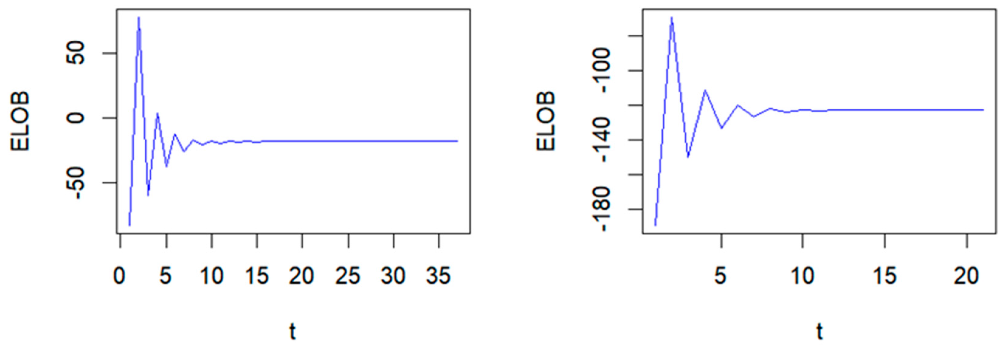
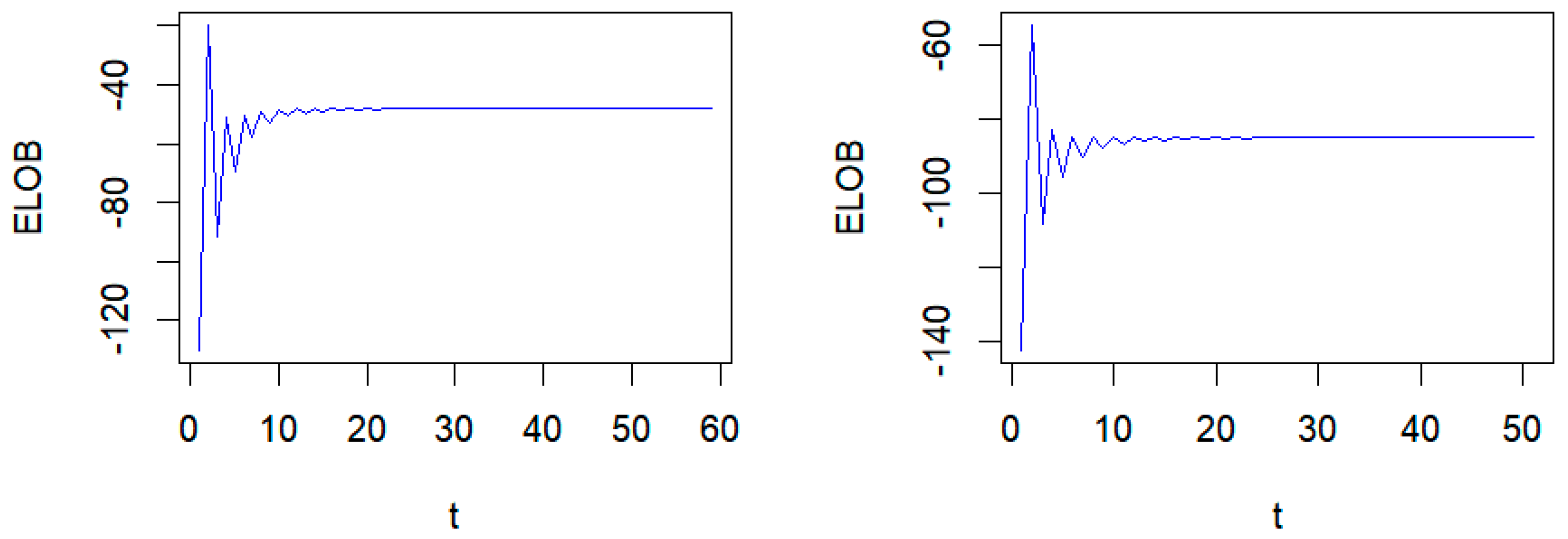
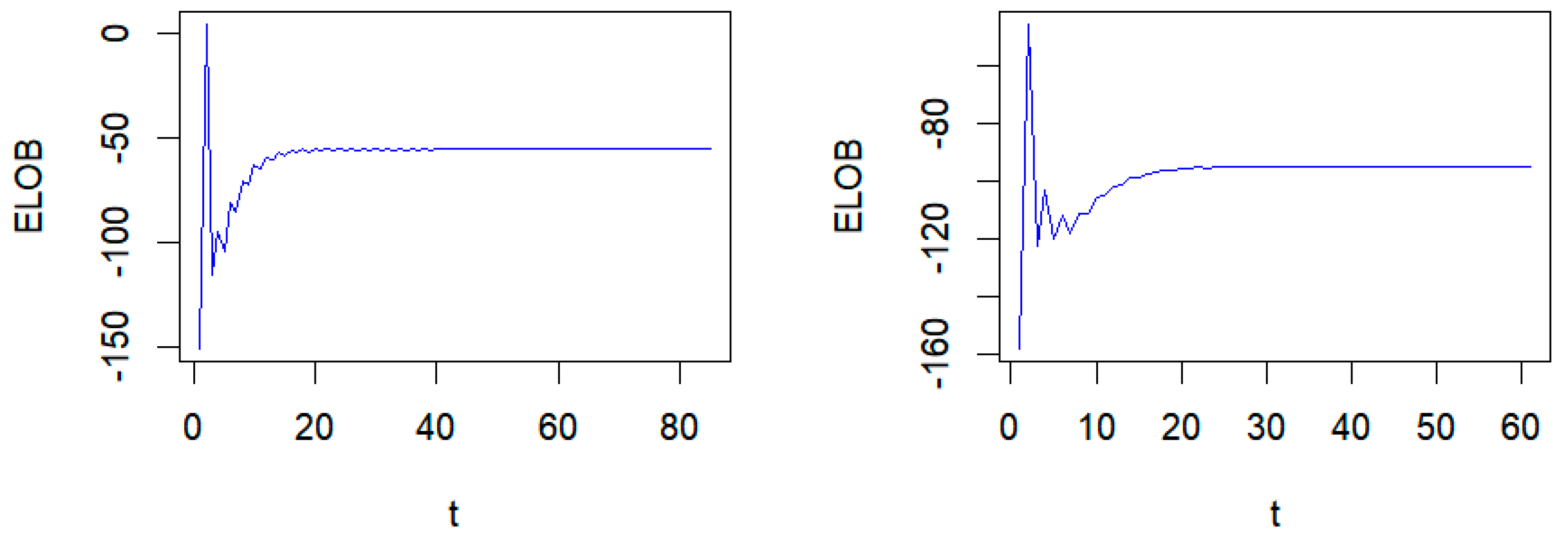
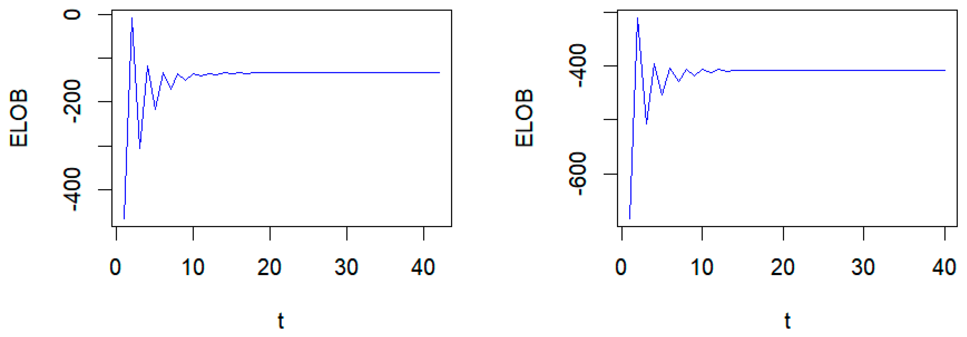
Figure 2, Figure 3, Figure 4 and Figure 5 display the results of the EMVB algorithm in computing the ELOB for τ = 0.5 in the four simulations (Left: ε i j ~ N   ( 0,1 ) ; Right: ε i j ~   C   ( 0,1 ) ). It can be observed that the EMVB algorithm converges after several iterations in all the cases. The GBEM algorithm requires multiple samples to ensure the accuracy of the computation, leading to a longer runtime.
The proposed VBEM algorithm for Bayesian quantile regression in linear mixed effects models offers several advantages over established methods, such as MCMC-based approaches. One of the main advantages of the VBEM algorithm is its significant reduction in computational time compared to MCMC-based methods, like GBEM and BQRLM. MCMC methods are known to be computationally expensive, especially for large datasets or high-dimensional models, while the VBEM algorithm provides a faster alternative due to its variational approximation framework. VBEM’s faster convergence and lower computational costs make it highly scalable, which is crucial for analyzing high-dimensional data or complex models with many covariates. Like Bayesian methods, VBEM effectively handles the sparsity inherent in high-dimensional data by selecting relevant variables. It also achieves this while providing good parameter estimates, making it a strong choice for variable selection tasks. By operating within a Bayesian framework, VBEM inherits the ability to quantify uncertainty and provide posterior distributions for all the submodels, which is an advantage over frequentist methods, like LASSO and SCAD, that only focus on point estimates.
A limitation of VBEM is that it is an approximate method, which can result in underestimating parameter variance. This is reflected in its slightly higher mean squared error (MSE) compared to MCMC-based methods. The trade-off for increased speed is a loss in the precision of the parameter uncertainty estimates.
We also estimate the hyperparameters in the NBP prior. In Simulation 1 and Simulation 4, where the sparsity level of β is the same (10% non-zero elements), the estimated hyperparameters are close: a = 0.125 , b = 0.607 (in Simulation 1) and a = 0.122 , b = 0.62 (in Simulation 4). In Simulation 2 and Simulation 3, as the number of non-zero elements in β increases, the hyperparameter estimates also increase: a = 0.515 , b = 0.311 ;   a = 19.885 , b = 1.189 .
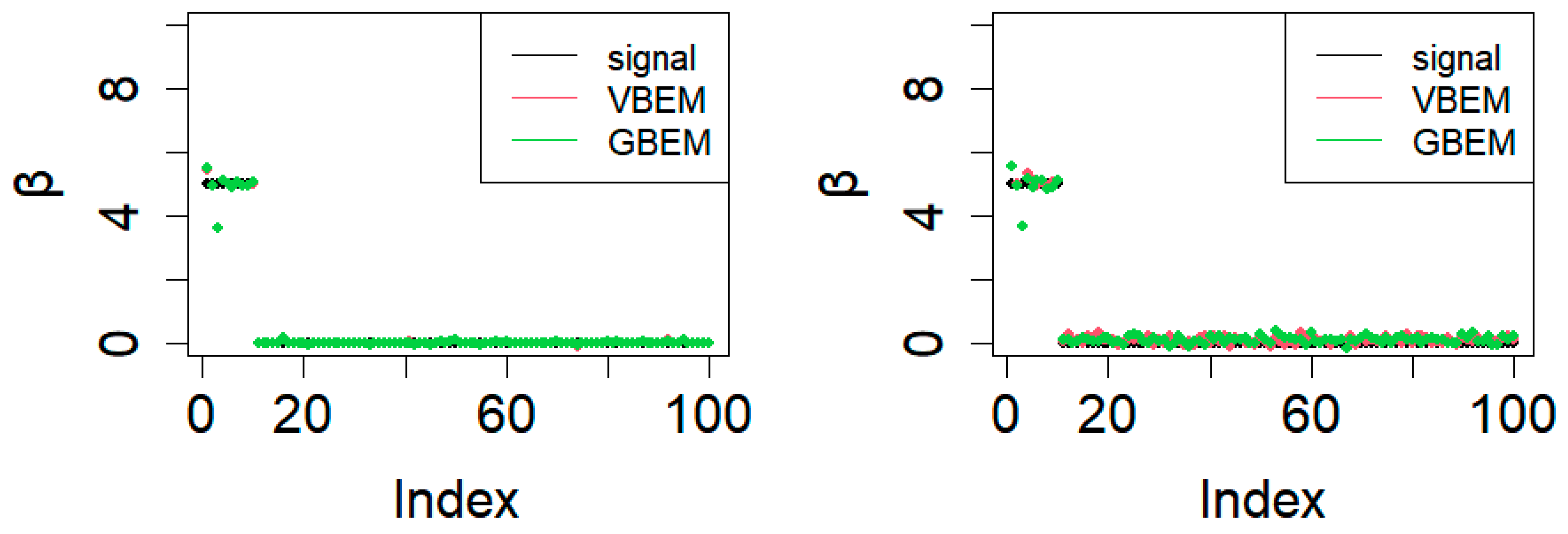
When τ = 0.5 , Figure 6 (Left: ε i j ~ N   ( 0,1 ) ; Right: ε i j ~   C   ( 0,1 ) ) presents the estimation results of the EMVB algorithm and the GBEM algorithm in Simulation 4. The true values of the signal β are shown in black. These findings further illustrate that there is little difference between the estimation results of the two algorithms. However, when ε i j ~   C   ( 0,1 ) , the performance of both the EMVB algorithm and the GBEM algorithm declines.

5. Real Data Analysis

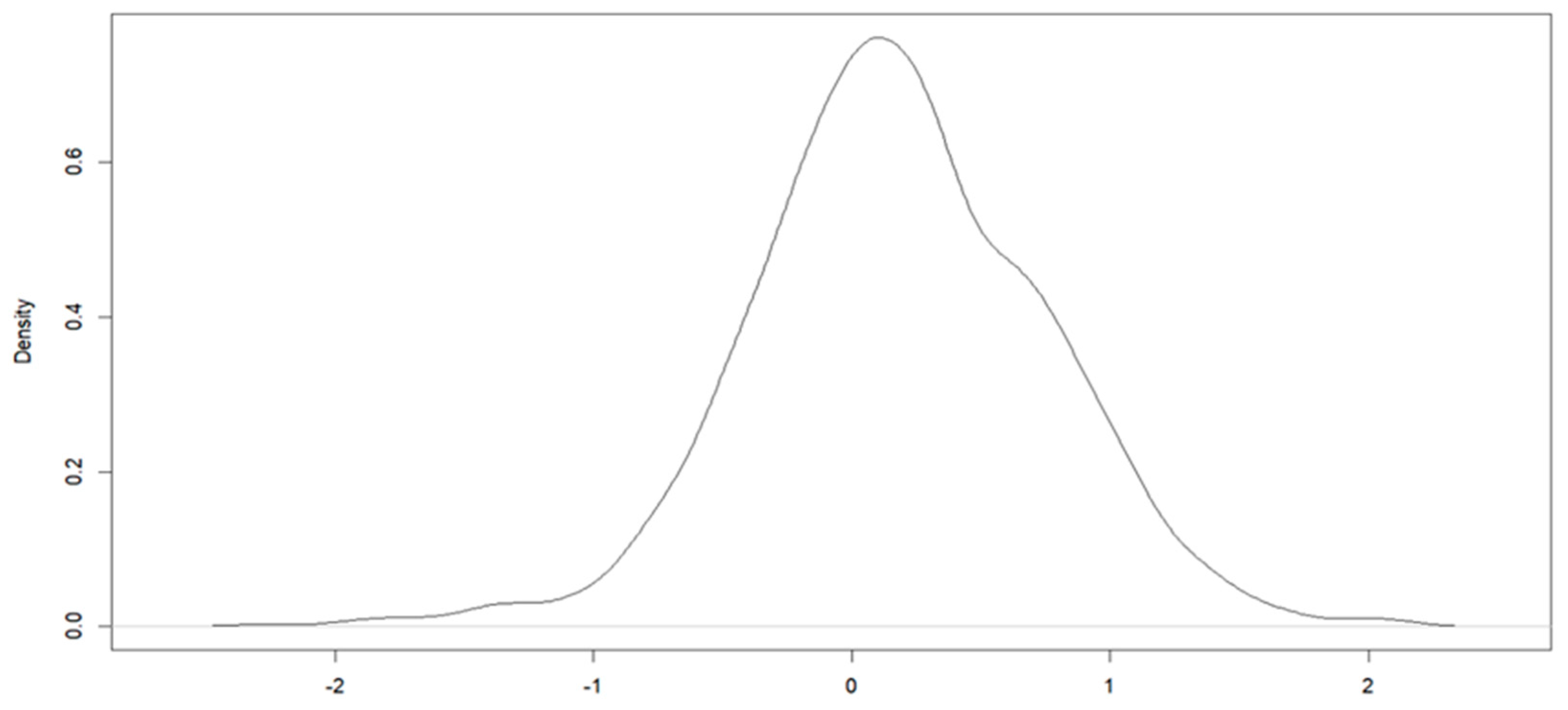
We applied the VBEM algorithm to the yeast cell cycle gene expression dataset collected from the CDC15 experiment [23]. The cell cycle process is typically divided into the M/G1-G1-S-G2-M phases. To better understand the phenomena behind the cell cycle process, it is important to identify the transcription factors (TFs) that regulate the expression levels of genes. Similar to Wang et al. [24], we analyzed a subset of the data corresponding to the G1 phase. The dataset can be obtained by loading the R package PGEE and using the command “data (“yeastG1”)”. It contains 1132 observations (283 genes, observed four times each) and 99 variables (e.g., id, y, time, and 96 TFs). The response variable y i j represents the log-transformed gene expression level of the gene,   i , at the time, j , and Figure 7 shows the density of the response variable. X i p is the matching score of the binding probability of the p th transcription factor on the promoter region of the i th gene. The binding probability is calculated using a mixture modeling approach based on ChIP binding experimental data, as detailed in Wang et al. [24]. We modeled it with the following formulation:
y i j = α 0 + α 1 t i j + p = 1 96 β p X i p + ε i j , i = 1,2 , , 283 , j = 1,2 , , 4 .
When τ = 0.25 ,   0.5 ,   o r   0.75 , the number of the TFs selected by the VBEM algorithm are 22, 16, and 12, respectively, and the specific TFs are listed in Table 9. Additionally, Table 9 also shows the TFs selected by the Penalized Generalized Estimating Equations (PGEE) method proposed by Wang [24]. At τ = 0.5 , the TFs selected by the VBEM algorithm are nearly identical to those selected by the PGEE method. While we used the DSS method to select the TFs, the PGEE method selected TFs with estimated coefficients greater than 10−3. In a real data analysis, we could not directly compare which variable selection method was better, but it was observed that the runtime of the VBEM algorithm was significantly shorter than that of the PGEE method.

6. Conclusions

In this paper, the primary contribution is the extension of the NBP prior to Bayesian quantile regression for linear mixed effects models, which improves the ability to perform Bayesian variable selection. The use of the VBEM algorithm for hyperparameter estimation in the NBP prior is another major innovation, offering a more computationally efficient alternative to traditional methods, like MCMC.
Our key findings include the following: (1) The VBEM algorithm is significantly faster than GBEM and other methods, especially when dealing with high-dimensional data, making it well-suited for large datasets and complex models. (2) While the VBEM algorithm tends to have a slightly higher mean squared error (MSE) due to its approximate nature, its performance in variable selection and predictive accuracy remains strong. (3) Bayesian methods, particularly those employing the VBEM algorithm, demonstrated superior predictive performance with a lower median mean absolute deviation (MMAD) compared to non-Bayesian methods.
The loss function of quantile regression is non-differentiable at the origin, which presents challenges for certain theoretical analyses. This limitation has been acknowledged as a major difficulty in applying VBEM to quantile regression. Unlike MCMC methods, Variational Bayesian methods (including VBEM) lack the same level of theoretical guarantees. The theoretical research on VBEM, particularly for quantile regression, is limited, making it more challenging to justify its use in some contexts where rigorous theoretical backing is required.
The proposed VBEM algorithm has substantial practical relevance for real-world decision making in fields such as genomics, finance, and healthcare, where high-dimensional data and complex models are common. The ability to quickly and accurately identify important variables while maintaining computational efficiency makes it a valuable tool for large-scale data analysis. By reducing computation time without sacrificing predictive power, the VBEM algorithm provides a practical solution for researchers and practitioners who require both accuracy and speed in data modeling and decision making.
The normal-beta prime prior can be applied to more complex and flexible models, such as nonparametric regression quantile regression or semiparametric quantile regression with unknown error distributions. The normal-beta prime prior can also be applied to other statistical problems, such as density estimation or classification tasks. With the rise of deep learning, researchers have begun to integrate deep learning models with Variational Bayesian methods to handle high-dimensional, nonlinear, and complex data. In quantile regression, deep neural networks can be employed to model the quantile function, and Variational Bayesian inference can be used to estimate the posterior distribution of the network parameters.

Author Contributions

The first two authors contributed equally to this work. M.T. contributed to the conceptualization, project administration, and funding acquisition for this project, with assistance from the corresponding author. All authors have read and agreed to the published version of the manuscript.

Funding

This research was supported by the Beijing Natural Science Foundation (1242005).

Data Availability Statement

The researchers can download the yeastG1 dataset from the R package “PGEE”.

Conflicts of Interest

The authors declare no conflicts of interest.

References

  1. Giraud, C. Introduction to High-Dimensional Statistics; Chapman and Hall/CRC: Boca Raton, FL, USA, 2021. [Google Scholar]
  2. Koenker, R. Quantile regression for longitudinal data. J. Multivar. Anal. 2004, 91, 74–89. [Google Scholar] [CrossRef]
  3. Yu, K.; Moyeed, R.A. Bayesian quantile regression. Stat. Probab. Lett. 2001, 54, 437–447. [Google Scholar] [CrossRef]
  4. Luo, Y.; Lian, H.; Tian, M. Bayesian quantile regression for longitudinal data models. J. Stat. Comput. Simul. 2012, 82, 1635–1649. [Google Scholar] [CrossRef]
  5. Sriram, K.; Shi, P.; Ghosh, P. A Bayesian Semiparametric Quantile Regression Model for Longitudinal Data with Application to Insurance Company Costs. IIM Bangalore Res. Pap. 2011, 355. [Google Scholar] [CrossRef]
  6. Chen, C.W.S.; Dunson, D.B.; Reed, C.; Yu, K. Bayesian variable selection in quantile regression. Stat. Its Interface 2013, 6, 261–274. [Google Scholar] [CrossRef]
  7. Alhamzawi, R.; Yu, K.; Benoit, D.F. Bayesian adaptive Lasso quantile regression. Stat. Model. 2012, 12, 279–297. [Google Scholar] [CrossRef]
  8. Li, Q.; Lin, N.; Xi, R. Bayesian regularized quantile regression. Bayesian Anal. 2010, 5, 533–556. [Google Scholar] [CrossRef]
  9. Ji, Y.; Shi, H. Bayesian variable selection in linear quantile mixed models for longitudinal data with application to macular degeneration. PLoS ONE 2020, 15, e0241197. [Google Scholar] [CrossRef] [PubMed]
  10. Huang, X.; Wang, J.; Liang, F. A Variational Bayesian algorithm for Bayesian variable selection. arXiv 2016, arXiv:1602.07640. [Google Scholar]
  11. Neville, S.E. Elaborate Distribution Semiparametric Regression via Mean Field Variational Bayesian Bayes. Ph.D. Thesis, University of Wollongong, Wollongong, Australia, 2013. [Google Scholar]
  12. Lim, D.; Park, B.; Nott, D.; Wang, X.; Choi, T. Sparse signal shrinkage and outlier detection in high-dimensional quantile regression with Variational Bayesian Bayes. Stat. Its Interface 2020, 13, 237–249. [Google Scholar] [CrossRef]
  13. Ray, K.; Szabó, B. Variational Bayesian Bayes for high-dimensional linear regression with sparse priors. J. Am. Stat. Assoc. 2022, 117, 1270–1281. [Google Scholar] [CrossRef]
  14. Ray, K.; Szabó, B.; Clara, G. Spike and slab Variational Bayesian Bayes for high dimensional logistic regression. arXiv 2010, arXiv:2010.11665. [Google Scholar]
  15. Blei, D.M.; Kucukelbir, A.; McAuliffe, J.D. Variational Bayesian inference: A review for statisticians. J. Am. Stat. Assoc. 2017, 112, 859–877. [Google Scholar] [CrossRef]
  16. Dai, D.; Tang, A.; Ye, J. High-Dimensional variable selection for quantile regression based on variational method. Mathematics 2023, 11, 2232. [Google Scholar] [CrossRef]
  17. Wang, Z.; Wu, Y.; Cheng, W. Variational inference on a Bayesian adaptive lasso Tobit quantile regression model. Stat 2023, 12, e563. [Google Scholar] [CrossRef]
  18. Li, X.; Tuerde, M.; Hu, X. Variational Bayesian Inference for Quantile Regression Models with Nonignorable Missing Data. Mathematics 2023, 11, 3926. [Google Scholar] [CrossRef]
  19. Bai, R.; Ghosh, M. On the beta prime prior for scale parameters in high-dimensional bayesian regression models. Stat. Sin. 2021, 31, 843–865. [Google Scholar] [CrossRef]
  20. Kozumi, H.; Kobayashi, G. Gibbs sampling methods for Bayesian quantile regression. J. Stat. Comput. Simul. 2011, 81, 1565–1578. [Google Scholar] [CrossRef]
  21. Hahn, P.R.; Carvalho, C.M. Decoupling shrinkage and selection in bayesian linear models: A posterior summary perspective. J. Am. Stat. Assoc. 2015, 110, 435–448. [Google Scholar] [CrossRef]
  22. Friedman, J.; Hastie, T.; Tibshirani, R. Regularization paths for generalized linear models via coordinate descent. J. Stat. Softw. 2010, 33, 1–22. [Google Scholar] [CrossRef]
  23. Eisen, M.B.; Spellman, P.T.; Brown, P.O.; Botstein, D. Cluster analysis and display of genome-wide expression patterns. Proc. Natl. Acad. Sci. USA 1998, 95, 14863–14868. [Google Scholar] [CrossRef] [PubMed]
  24. Wang, L.; Zhou, J.; Qu, A. Penalized generalized estimating equations for high-dimensional longitudinal data analysis. Biometrics 2011, 68, 353–360. [Google Scholar] [CrossRef] [PubMed]
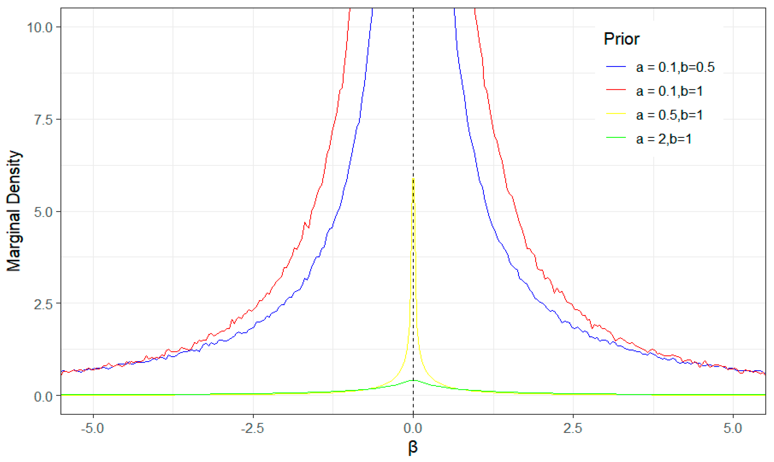
Figure 1. The density of the beta prime prior for various values of ( a , b ) .
Mathematics 12 03311 g001
Figure 2. ELOB of the EMVB algorithm for Simulation 1 ((Left): ε i j ~ N   ( 0,1 ) ; (Right): ε i j ~   C   ( 0,1 ) ).
Mathematics 12 03311 g002
Figure 3. ELOB of the EMVB algorithm for Simulation 2 ((Left): ε i j ~ N   ( 0,1 ) ; (Right): ε i j ~   C   ( 0,1 ) ).
Mathematics 12 03311 g003
Figure 4. ELOB of the EMVB algorithm for Simulation 3 ((Left): ε i j ~ N   ( 0,1 ) ; (Right): ε i j ~   C   ( 0,1 ) ).
Mathematics 12 03311 g004
Figure 5. ELOB of the EMVB algorithm for Simulation 4 ((Left): ε i j ~ N   ( 0,1 ) ; (Right): ε i j ~   C   ( 0,1 ) ).
Mathematics 12 03311 g005
Figure 6. Comparison of the EMVB algorithm and the GBEM algorithm for Simulation 4.
Mathematics 12 03311 g006
Figure 7. The density of the log-transformed gene expression levels.
Mathematics 12 03311 g007
Table 1. Comparison of Simulation 1 ( ε i j ~ N   ( 0,1 ) ).
τMethodMSEMMADTPRFDRT
0.25VBEM3.20 (0.19)1.42 (0.25)1.00 (0.00)0.00 (0.00)0.35 (0.06)
GBEM3.19 (0.24)1.44 (0.16)1.00 (0.00)0.00 (0.00)17.61 (1.52)
BQRLM3.44 (0.23)1.52 (0.28)1.00 (0.00)0.00 (0.00)15.26 (1.02)
QRM3.32 (0.33)2.55 (0.48)1.00 (0.00)0.95 (0.13)0.36 (0.12)
QRML3.24 (0.23)2.35 (0.38)1.00 (0.00)0.04 (0.01)0.46 (0.09)
0.5VBEM3.08 (0.34)1.12 (0.14)1.00 (0.00)0.00 (0.00)0.26 (0.05)
GBEM3.15 (0.21)1.38 (0.17)1.00 (0.00)0.00 (0.00)17.45 (1.45)
BQRLM3.35 (0.21)1.49 (0.32)1.00 (0.00)0.00 (0.00)14.26 (1.52)
QRM3.25 (0.42)2.46 (0.18)1.00 (0.00)0.93 (0.10)0.25 (0.14)
QRML3.20 (0.23)2.33 (0.29)1.00 (0.00)0.06 (0.02)0.45 (0.06)
0.75VBEM3.21 (0.32)1.44 (0.30)1.00 (0.00)0.00 (0.00)0.39 (0.02)
GBEM3.18 (0.19)1.46 (0.15)1.00 (0.00)0.00 (0.00)17.04 (1.02)
BQRLM3.40 (0.23)1.55 (0.31)1.00 (0.00)0.00 (0.00)15.33 (1.05)
QRM3.49 (0.29)2.48 (0.41)0.98 (0.03)0.94 (0.02)0.33 (0.11)
QRML3.38 (0.23)2.39 (0.38)1.00 (0.00)0.08 (0.02)0.48 (0.10)
Table 2. Comparison of Simulation 1 ( ε i j ~   C   ( 0,1 ) ).
τMethodMSEMMADTPRFDRT
0.25VBEM5.50 (0.27)2.85 (0.35)1.00 (0.00)0.00 (0.00)0.45 (0.09)
GBEM5.32 (0.45)2.94 (0.16)1.00 (0.00)0.00 (0.00)18.73 (1.33)
BQRLM6.47 (0.35)3.12 (0.18)1.00 (0.00)0.00 (0.00)16.39 (1.52)
QRM5.92 (0.42)4.59 (0.40)1.00 (0.00)0.91 (0.12)0.39 (0.22)
QRML5.84 (0.23)4.27 (0.29)1.00 (0.00)0.03 (0.01)0.52 (0.05)
0.5VBEM5.48 (0.21)2.62 (0.18)1.00 (0.00)0.00 (0.00)0.29 (0.06)
GBEM5.75 (0.21)2.48 (0.17)1.00 (0.00)0.00 (0.00)17.46 (1.63)
BQRLM6.15 (0.20)2.69 (0.27)1.00 (0.00)0.00 (0.00)13.63 (1.01)
QRM5.87 (0.39)3.16 (0.18)1.00 (0.00)0.92 (0.12)0.27 (0.11)
QRML5.79 (0.23)3.03 (0.29)1.00 (0.00)0.07 (0.01)0.49 (0.07)
0.75VBEM5.53 (0.25)2.87 (0.39)1.00 (0.00)0.00 (0.00)0.46 (0.09)
GBEM5.62 (0.45)2.98 (0.16)1.00 (0.00)0.00 (0.00)19.06 (1.33)
BQRLM6.37 (0.33)3.15 (0.16)1.00 (0.00)0.00 (0.00)18.22 (1.02)
QRM5.98 (0.52)4.61 (0.37)1.00 (0.00)0.94 (0.11)0.38 (0.24)
QRML5.74 (0.23)4.07 (0.22)1.00 (0.00)0.02 (0.01)0.51 (0.03)
Table 3. Comparison of Simulation 2 ( ε i j ~ N   ( 0,1 ) ).
τMethodMSEMMADTPRFDRT
0.25VBEM3.69 (0.17)1.46 (0.21)1.00 (0.00)0.00 (0.00)0.38 (0.04)
GBEM3.55 (0.16)1.42 (0.15)1.00 (0.00)0.00 (0.00)16.61 (0.14)
BQRLM3.64 (0.25)1.55 (0.28)1.00 (0.00)0.00 (0.00)16.33 (1.05)
QRM3.74 (0.33)2.45 (0.31)1.00 (0.00)0.94 (0.10)0.41 (0.15)
QRML3.66 (0.23)2.13 (0.38)1.00 (0.00)0.04 (0.02)0.43 (0.06)
0.5VBEM2.88 (0.27)1.33 (0.29)1.00 (0.00)0.00 (0.00)0.37 (0.04)
GBEM2.94 (0.31)1.35 (0.15)1.00 (0.00)0.00 (0.00)17.26 (1.15)
BQRLM3.09 (0.21)1.52 (0.35)1.00 (0.00)0.00 (0.00)16.52 (1.02)
QRM3.33 (0.29)2.39 (0.15)1.00 (0.00)0.92 (0.10)0.29 (0.10)
QRML3.25 (0.21)2.28 (0.29)1.00 (0.00)0.05 (0.02)0.41 (0.06)
0.75VBEM3.22 (0.39)1.49 (0.25)1.00 (0.00)0.00 (0.00)0.35 (0.03)
GBEM3.19 (0.16)1.45 (0.11)1.00 (0.00)0.00 (0.00)18.06 (1.16)
BQRLM3.42 (0.29)1.57 (0.30)1.00 (0.00)0.00 (0.00)15.49 (1.18)
QRM3.41 (0.29)2.45 (0.35)0.96 (0.02)0.92 (0.02)0.31 (0.21)
QRML3.35 (0.26)2.37 (0.31)1.00 (0.00)0.05 (0.02)0.45 (0.20)
Table 4. Comparison of Simulation 2 ( ε i j ~   C   ( 0,1 ) ).
τMethodMSEMMADTPRFDRT
0.25VBEM6.61 (0.35)2.96 (0.22)1.00 (0.00)0.00 (0.00)0.47 (0.09)
GBEM6.16 (0.45)3.13 (0.15)1.00 (0.00)0.00 (0.00)17.77 (0.28)
BQRLM6.43 (0.30)3.25 (0.21)1.00 (0.00)0.00 (0.00)15.39 (1.02)
QRM6.95 (0.40)4.38 (0.45)1.00 (0.00)0.90 (0.11)0.35 (0.21)
QRML6.82 (0.15)4.17 (0.29)1.00 (0.00)0.02 (0.01)0.55 (0.04)
0.5VBEM5.85 (0.25)2.52 (0.15)1.00 (0.00)0.00 (0.00)0.28 (0.07)
GBEM5.96 (0.25)2.33 (0.11)1.00 (0.00)0.00 (0.00)17.05 (0.47)
BQRLM6.14 (0.20)2.61 (0.21)1.00 (0.00)0.00 (0.00)12.98 (1.11)
QRM5.99 (0.34)3.01 (0.29)1.00 (0.00)0.90 (0.10)0.25 (0.10)
QRML5.89 (0.21)3.12 (0.20)1.00 (0.00)0.09 (0.01)0.38 (0.08)
0.75VBEM6.08 (0.32)2.92 (0.31)1.00 (0.00)0.00 (0.00)0.47 (0.08)
GBEM6.21 (0.45)2.82 (0.14)1.00 (0.00)0.00 (0.00)19.33 (1.02)
BQRLM6.39 (0.36)3.18 (0.11)1.00 (0.00)0.00 (0.00)19.20 (1.01)
QRM6.32 (0.32)4.55 (0.32)1.00 (0.00)0.90 (0.15)0.40 (0.25)
QRML6.36 (0.23)4.15 (0.25)1.00 (0.00)0.03 (0.01)0.55 (0.02)
Table 5. Comparison of Simulation 3 ( ε i j ~ N   ( 0,1 ) ).
τMethodMSEMMADTPRFDRT
0.25VBEM3.63 (0.15)1.40 (0.25)1.00 (0.00)/0.38 (0.04)
GBEM3.42 (0.19)1.36 (0.14)1.00 (0.00)/16.63 (0.22)
BQRLM3.69 (0.28)1.58 (0.33)1.00 (0.00)/17.55 (1.21)
QRM3.70 (0.28)2.51 (0.35)1.00 (0.00)/0.36 (0.22)
QRML3.87 (0.19)2.59 (0.21)1.00 (0.00)/0.41 (0.05)
0.5VBEM2.76 (0.23)1.35 (0.29)1.00 (0.00)/0.35 (0.02)
GBEM2.78 (0.18)1.38 (0.19)1.00 (0.00)/16.77 (0.61)
BQRLM3.28 (0.21)1.49 (0.22)1.00 (0.00)/17.02 (1.52)
QRM3.01 (0.18)2.51 (0.19)1.00 (0.00)/0.24 (0.03)
QRML3.39 (0.19)2.62 (0.27)1.00 (0.00)/0.47 (0.05)
0.75VBEM3.73 (0.23)1.52 (0.22)1.00 (0.00)/0.53 (0.09)
GBEM3.56 (0.25)1.55 (0.19)1.00 (0.00)/17.73 (1.28)
BQRLM3.82 (0.20)1.66 (0.25)1.00 (0.00)/15.33 (1.06)
QRM3.61 (0.29)2.37 (0.35)1.00 (0.00)/0.35 (0.02)
QRML3.66 (0.25)2.52 (0.23)1.00 (0.00)/0.41 (0.12)
Table 6. Comparison of Simulation 3 ( ε i j ~   C   ( 0,1 ) ).
τMethodMSEMMADTPRFDRT
0.25VBEM6.52 (0.26)2.98 (0.23)1.00 (0.00)/0.47 (0.09)
GBEM6.04 (0.15)3.09 (0.17)1.00 (0.00)/18.93 (0.21)
BQRLM6.48 (0.22)3.07 (0.29)1.00 (0.00)/16.33 (1.21)
QRM6.56 (0.33)4.01 (0.36)1.00 (0.00)/0.39 (0.15)
QRML6.77 (0.15)4.59 (0.29)1.00 (0.00)/0.50 (0.04)
0.5VBEM5.32 (0.22)2.69 (0.18)1.00 (0.00)/0.35 (0.05)
GBEM5.59 (0.25)2.52 (0.21)1.00 (0.00)/17.59 (1.23)
BQRLM6.09 (0.36)2.77 (0.21)1.00 (0.00)/14.15 (1.35)
QRM5.84 (0.34)3.32 (0.19)1.00 (0.00)/0.30 (0.09)
QRML5.74 (0.21)3.47 (0.15)1.00 (0.00)/0.36 (0.05)
0.75VBEM6.11 (0.52)2.85 (0.29)1.00 (0.00)/0.45 (0.06)
GBEM6.39 (0.32)2.78 (0.11)1.00 (0.00)/18.36 (1.05)
BQRLM6.35 (0.31)3.26 (0.28)1.00 (0.00)/19.41 (1.55)
QRM6.18 (0.39)4.05 (0.25)1.00 (0.00)/0.35 (0.21)
QRML6.26 (0.18)4.01 (0.35)1.00 (0.00)/0.53 (0.10)
Table 7. Comparison of Simulation 4 ( ε i j ~ N   ( 0,1 ) ).
τMethodMSEMMADTPRFDRT
0.25VBEM4.13 (0.18)1.92 (0.35)1.00 (0.00)0.00 (0.00)2.45 (0.12)
GBEM4.02 (0.12)1.88 (0.15)1.00 (0.00)0.00 (0.00)63.52 (2.69)
BQRLM4.61 (0.23)2.18 (0.26)1.00 (0.00)0.00 (0.00)65.54 (1.32)
QRM4.62 (0.35)2.85 (0.42)1.00 (0.00)1.00 (0.00)0.89 (0.25)
QRML4.22 (0.25)2.48 (0.36)1.00 (0.00)0.00 (0.00)0.92 (0.09)
0.5VBEM2.92 (0.29)1.45 (0.33)1.00 (0.00)0.00 (0.00)1.49 (0.09)
GBEM2.72 (0.25)1.44 (0.14)1.00 (0.00)0.00 (0.00)64.41 (2.69)
BQRLM3.05 (0.19)1.54 (0.22)1.00 (0.00)0.00 (0.00)67.33 (1.35)
QRM3.22 (0.29)2.08 (0.13)1.00 (0.00)1.00 (0.00)0.85 (0.05)
QRML3.84 (0.11)2.59 (0.17)1.00 (0.00)0.00 (0.00)0.88 (0.05)
0.75VBEM4.39 (0.15)1.73 (0.15)1.00 (0.00)0.00 (0.00)2.53 (0.52)
GBEM4.19 (0.21)1.75 (0.25)1.00 (0.00)0.00 (0.00)64.73 (2.35)
BQRLM4.22 (0.17)1.80 (0.25)1.00 (0.00)0.00 (0.00)69.21 (1.89)
QRM4.42 (0.18)2.08 (0.38)1.00 (0.00)1.00 (0.00)0.92 (0.11)
QRML4.62 (0.22)2.35 (0.35)1.00 (0.00)0.00 (0.00)1.82 (0.25)
Table 8. Comparison of Simulation 4 ( ε i j ~   C   ( 0,1 ) ).
τMethodMSEMMADTPRFDRT
0.25VBEM5.95 (0.22)2.25 (0.21)1.00 (0.00)0.00 (0.00)3.66 (0.67)
GBEM6.21 (0.52)1.92 (0.18)1.00 (0.00)0.00 (0.00)70.47 (3.02)
BQRLM6.23 (0.36)2.42 (0.36)1.00 (0.00)0.00 (0.00)69.33 (1.58)
QRM6.55 (0.28)2.94 (0.35)1.00 (0.00)1.00 (0.00)0.92 (0.14)
QRML6.50 (0.27)2.82 (0.39)1.00 (0.00)0.00 (0.00)0.95 (0.09)
0.5VBEM4.98 (0.15)1.62 (0.32)1.00 (0.00)0.00 (0.00)2.89 (0.19)
GBEM4.93 (0.32)1.52 (0.21)1.00 (0.00)0.00 (0.00)68.17 (3.19)
BQRLM5.02 (0.33)1.65 (0.21)1.00 (0.00)0.00 (0.00)68.25 (1.98)
QRM5.51 (0.29)2.74 (0.29)1.00 (0.00)1.00 (0.00)0.88 (0.07)
QRML5.41 (0.32)2.55 (0.13)1.00 (0.00)0.00 (0.00)0.92 (0.12)
0.75VBEM6.89 (0.39)1.82 (0.19)1.00 (0.00)0.00 (0.00)3.92 (0.66)
GBEM7.14 (0.21)1.88 (0.13)1.00 (0.00)0.00 (0.00)71.55 (4.055)
BQRLM7.20 (0.63)2.05 (0.21)1.00 (0.00)0.00 (0.00)72.25 (1.33)
QRM8.05 (0.56)2.89 (0.42)1.00 (0.00)1.00 (0.00)0.95 (0.15)
QRML7.60 (0.19)2.46 (0.34)1.00 (0.00)0.00 (0.00)1.76 (0.32)
Table 9. Comparison of the VBEM algorithm and the PGEE method on yeast cell cycle gene expression data.
MethodThe Selected TFsT
VBEM
( τ = 0.25 )
“ABF1”“ARG81”“ASH1”“FKH1”“FKH2”“GAT3” “GCR1”“GCR2”“GTS1”“HMS1”“MBP1”“MET4” “MSN4”“NDD1”“ROX1”“SIP4”“STB1”“STP1” “SWI4”“SWI6”“YAP6” “ZAP1”156.36
VBEM
( τ = 0.5 )
“ABF1”“ARG81”“ASH1”“FKH2”“GAT3”“GCR2”
“MBP1”“MET4”“MSN4”“NDD1”“ROX1”“STB1”
“STP1”“SWI4”“SWI6”“YAP6”
159.63
VBEM
( τ = 0.75 )
“ABF1”“ASH1”“FKH2”“GAT3”“GCR2”“MBP1” “MSN4”“NDD1”“STB1”“STP1”“SWI4”“SWI6”159.61
PGEE“ABF1”“FKH1”“FKH2”“GAT3”“GCR2”“MBP1” “MSN4”“NDD1”“PHD1”“RGM1”“RLM1”“SMP1”
“SRD1”“STB1”“SWI4”“SWI6”
1331.59
Disclaimer/Publisher’s Note: The statements, opinions and data contained in all publications are solely those of the individual author(s) and contributor(s) and not of MDPI and/or the editor(s). MDPI and/or the editor(s) disclaim responsibility for any injury to people or property resulting from any ideas, methods, instructions or products referred to in the content.