Abstract
This article is devoted to the mathematical analysis of a heat and mass transfer model for the pressure-induced flow of a viscous fluid through a plane channel subject to Navier’s slip conditions on the channel walls. The important feature of our work is that the used model takes into account the effects of variable viscosity, thermal conductivity, and slip length, under the assumption that these quantities depend on temperature. Therefore, we arrive at a boundary value problem for strongly nonlinear ordinary differential equations. The existence and uniqueness of a solution to this problem is analyzed. Namely, using the Galerkin scheme, the generalized Borsuk theorem, and the compactness method, we proved the existence theorem for both weak and strong solutions in Sobolev spaces and derive some of their properties. Under extra conditions on the model data, the uniqueness of a solution is established. Moreover, we considered our model subject to some explicit formulae for temperature dependence of viscosity, which are applied in practice, and constructed corresponding exact solutions. Using these solutions, we successfully performed an extra verification of the algorithm for finding solutions that was applied by us to prove the existence theorem.
Keywords:
heat and mass transfer model; viscous fluid; Poiseuille flow; Navier slip condition; nonlinear boundary value problem; variable coefficients; weak and strong solutions; exact solutions; Galerkin method; existence and uniqueness theorem MSC:
76D03; 34A34; 34A05
1. Introduction
Flow and heat transfer in a channel, a tube, or a pipeline, containing a non-uniformly heated moving fluid or a gas, is one of the most common situations encountered in engineering practice. This paper deals with the nonlinear heat and mass transfer model describing the steady unidirectional pressure-driven flow of an incompressible viscous fluid in the channel between the two fixed plates under Navier-type slip (in other terminology, “free slip”) boundary conditions and Robin’s conditions for the heat flux on the channel walls:
where
- is the velocity component in the x-direction;
- is the deviation from the reference temperature;
- is the pressure gradient along the x-direction (), that is, ;
- is the viscosity coefficient, ;
- is the thermal conductivity coefficient, ;
- is the heat source intensity;
- is the heat transfer coefficient, ;
- is the friction coefficient, ;
- the symbol ′ denotes the differentiation with respect to y.
The flow configuration is shown in Figure 1. In the literature, this kind of fluid flow is commonly referred to as the “plane Poiseuille flow”.
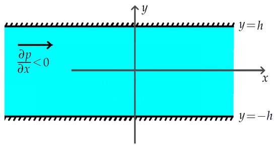
Figure 1.
Fluid flow between the fixed plates driven by a given pressure gradient .
When studying model (1), we suppose that and are unknown functions, while all the other functions and constants are given.
For the sake of simplicity, in the following it will be assumed that the function , describing the heat source intensity, is even. Thus, the model under consideration has the symmetry property with respect to the plane .
The main feature of the present paper is that we consider the heat and mass transfer model with variable coefficients, assuming that the viscosity , the thermal conductivity k, and the slip length depend on the temperature , and these dependencies are formulated in the most general form. In spite of the simplicity of formulation, problem (1) is challenging from a point of view of applying both analytical and numerical methods to it. The presence of variable coefficients in the model significantly complicates its theoretical study and requires the development of a special mathematical apparatus for constructing solutions of the corresponding boundary value problem (BVP). To overcome related difficulties, we will use some of the following authors’ findings and approaches [1,2,3].
Note that taking into account the dependence of physical properties of a fluid on temperature is critical for many applications. For example, it is important for engine lubricants, which should perform well under varying temperature conditions, cooling and heating systems, food processing, medical and biological sectors, pollution control, as well as wastewater treatment. Also, in studying many natural phenomena, it is needed to consider temperature-dependent properties of fluids. For example, for geysers and volcanic eruptions, the radius of impact on the environment of their plume is significantly influenced by temperature-dependent variable viscosity. For more detail, we refer to the papers [4,5,6,7].
Another feature of our work is that we use a nonlinear temperature-dependent Navier’s slip condition on the channel walls (see the pioneering work [8]) instead of the standard no-slip condition. Mathematically speaking, the zero Dirichlet condition for the velocity field is replaced by a nonlinear Robin condition. The motivation of this lies in covering situations in which fluids exhibit phenomena inconsistent with the assumption of no-slip [9]. In this regard, we can mention the cases when boundaries are rough [10], for instance, the skin of sharks or golf balls [11,12]. One more application of interest can also be found in drag control of aircraft wings; in order to reduce the drag, small injection jets are introduced over wings of planes [13]. In such cases, it is really important to introduce other interfacial conditions to adequately predict the behavior of a fluid on boundaries of a flow domain. A short survey of popular slip boundary conditions, among which the Navier condition occupies one of the central places, is given in [14].
The main aim of this paper is to give a comprehensive mathematical study of problem (1), primarily focusing on the existence and uniqueness theorems (for both the weak and strong formulations of this BVP) and algorithms for constructing solutions. We also establish some qualitative and quantitative properties of solutions. Moreover, considering our model under some (physically meaningful) analytical formulae for temperature dependence of viscosity, we construct corresponding solutions in an explicit form. These solutions favor a better understanding of the qualitative features of fluid flows with variable physical properties and can be used for verification of relevant approximate analytical and numerical methods.
It should be mentioned here that non-isothermal viscous flows through conduits having simple cross-section geometry with temperature-dependent viscosity has been studied by many authors in various aspects for both Newtonian and non-Newtonian fluids; see, for example, the papers [15,16,17,18,19,20,21,22,23,24,25,26,27,28,29] and the references therein. In most of these works, it is assumed that the fluid viscosity is given by Reynold’s model [30] (also known as the Nahme-type law [31]):
or by the power law equation [32]:
In the above relations, A, B, , , , and are substance-dependent constants. Sometimes the temperature-dependent viscosity and thermal conductivity are organized as a power series [33].
In the framework of the Stokes approximation, an unsteady flow problem for a non-uniformly heated fluid with constant viscosity under specified inflow–outflow regimes on parts of the boundary of the flow region was considered in [34]. The articles [35,36,37,38] and [39,40,41] are devoted to the study of BVPs for the generalized Boussinesq system with variable coefficients under the zero and non-zero Dirichlet boundary conditions for the velocity field, respectively. The initial-boundary value problem modeling an unsteady unidirectional convective flow of incompressible fluids in a vertical heat exchanger having an arbitrary cross section was studied in [42]. The paper [43] deals with a boundary control problem for the model describing the motion of a viscous heat conduction fluid under slip boundary conditions. Some models for complex heat transfer were investigated in the series of works [44,45,46,47]. The “complete” Boussinesq system involving the viscous dissipation, which is represented in the heat equation by the quadratic Rayleigh function, has been recently studied in [48,49,50,51,52]. We also mention the works [53,54,55,56,57,58], which are within the framework of the analytical approach to solving non-standard problems of hydrodynamics.
After this introduction, our article is organized as follows. In Section 2, we introduce the notations and needed function spaces, along with some important preliminary results such as the generalized Borsuk theorem (see Proposition 1), which will be used in proving the solvability of problem (1). Moving on to Section 3, we give both the weak and strong formulations of our BVP in suitable subspaces of Sobolev spaces. Section 4 contains the main results of this work—Theorems 1–3 about the existence, uniqueness, and properties of solutions to problem (1). These theorems are proved in Section 5. Finally, in Section 6, we construct some solutions in the closed form and, using them, perform an extra verification of the algorithm of finding solutions, developed by us to prove Theorem 1.
2. Preliminaries
2.1. Notations and Function Spaces
Let E and F be real Banach spaces. By denote the space of continuous linear mappings from E into F. This space is equipped with the operator norm
The symbol ↪ denotes a continuous embedding, while stands for a compact embedding.
The symbol ⇀ (→, ⇉, resp.) denotes weak (strong, uniform, resp.) convergence.
Let . For a function , by denote the mean of v, that is,
By denote the space of -smooth real-valued functions with compact support contained in the open interval .
For any , and , (, , resp.) denotes the Lebesgue (Sobolev, Hölder, resp.) space of real-valued functions defined on . Moreover, we will use the standard notation
By (, resp.) denote the space of continuous (absolutely continuous, resp.) functions on . Detailed descriptions of properties of these spaces can be found in the books [59,60,61].
We define a special scalar product in the Sobolev space by the formula:
The expediency of using this scalar product in solving our BVP will become clear in the following.
Note that any function belonging to the space is absolutely continuous and, moreover, the equality
holds. Therefore, we can naturally determine values of functions from at the endpoints and .
The following statement is useful in studying strong solutions.
Lemma 1.
If , then and
Further, let us formulate some results on the embedding of the space into Hölder’s spaces.
Lemma 2.
Suppose , then
- , for
- , for .
This lemma is a particular case of the Sobolev embedding theorem (see, for instance, [62], Chapter III, § 2.8).
Corollary 1.
Let and . If in as , then as .
For studying fluid flows that exhibit the symmetry property with respect to the plane , we introduce the following spaces:
Moreover, we also will use three subspaces of the Sobolev space :
which are Hilbert spaces with respect to the scalar product that is induced from .
It is easily shown that the following decomposition takes place:
where the symbol ⊕ denotes the orthogonal sum.
Consider the sequence , where
This sequence is an orthonormal basis of the space .
Lastly, let . Taking into account the decomposition (2), one can easily see that the sequence is an orthonormal basis of the space .
2.2. Embedding Operator
Lemma 3.
Let be the embedding operator. Then
Proof.
Suppose v is an arbitrary function from the space . Using the following representation
which holds due to the Newton–Leibniz formula for absolutely continuous functions, we derive
Moreover, applying Hölder’s inequality, we obtain
Since
we see that
or equivalently,
This yields the required estimate (4) for the norm of the embedding operator I. Thus, Lemma 3 is proved. □
2.3. Abstract Result on Solvability of One-Parameter Family of Equations
When proving the well-posedness of problem (1) by Galerkin’s scheme, we will need the following proposition.
Proposition 1
(Generalized Borsuk’s theorem). Let ρ be a positive number and let
Suppose is a family of mappings such that
- the mapping , is continuous;
- for any
- the mapping is linear.
Then, for any , the equation has at least one solution in the ball . In particular, the equation is solvable in this ball.
This abstract result can be proved by applying methods of the theory of topological degree [63,64].
3. Weak and Strong Solutions
In the sequel, we assume that the functions , , k, satisfy the following four conditions:
- (.1)
- the functions , , and are continuous;
- (.2)
- the strict inequalities and hold for any
- (.3)
- there exists a constant such that for any
- (.4)
- the function is even and belongs to the space .
Definition 1
(Weak solution). We shall say that a pair is a weak solution to problem (1) if
- for any test functions and , the following equalities hold:
It can easily be checked that any classical solution to problem (1) is a weak solution. On the other hand, if is a weak solution and the functions u, , , k are sufficiently smooth, then is a classical solution to this problem.
Definition 2
(Strong solution). We shall say that a pair is a strong solution to problem (1) if the following conditions hold:
- the equality holds almost everywhere in
- the equality holds almost everywhere in
- the four boundary conditions are true:
- ,
- ,
- ,
- .
Taking into account Lemma 1, we see that in the last definition. In particular, this means that values of these functions in the endpoints of are well defined. Therefore, the above boundary conditions, which contain these functions, are meaningful.
If is a strong solution of problem (1), then this solution is weak, but the converse statement is not true. However, under extra smoothness assumptions on the functions and k, a weak solution becomes a strong solution.
4. Main Results
4.1. Well-Posedness of BVP
In the following two theorems, we collect our results about the existence, uniqueness, and regularity of a solution to the BVP under consideration.
Theorem 1
(Existence and regularity). Suppose that conditions (.1)–(.4) hold. Then:
Theorem 2
(Uniqueness). If, in addition to conditions (.1)–(.4), we require that the function k satisfies the Lipschitz condition
with a positive constant such that
then problem (1) admits a unique weak solution.
4.2. Boundary Values of Solutions, Energy Equalities, and Extrema
The next theorem summarizes our results related to studying properties of weak and strong solutions to system (1).
Theorem 3
(Properties of solutions). Under the conditions of Theorem 1, the following statements hold.
5. Proof of Main Results
5.1. Proof of Theorem 1
We will prove the existence result (a) by the Galerkin method, using Proposition 1 and compactness arguments for an appropriate limit passage. For convenience, our proof is divided into three steps.
Step 1: Galerkin’s approximation. Let m be an arbitrary integer. Galerkin’s approximate solutions will be sought in the form
where is defined in (3), while and are unknown coefficients. To determine these coefficients, we consider a finite-dimensional problem with the parameter :
Find a vector such that the functions and satisfy the following equalities:
and
Step 2: A priori estimates of Galerkin’s solutions. Let us assume that satisfies relations (17) and (18) for some . Taking into account that is an orthonormal basis of the space , we obtain
Further, we multiply jth equality of system (18) by and sum up the results over j from 0 to m. This gives
Using the last relation, we derive
whence
Next, we multiply jth equality of system (17) by and sum up the results over j from 0 to m. As a result, we arrive at the following equality
In view of condition (.2), for any , we have
From (24) it follows that
Finally, combining relations (19), (20), and (25), we derive the estimate for the Euclidean norm of the vector :
It should be noticed at this point that the right-hand side of estimate (26) does not depend on the parameters m and t. Therefore, applying Proposition 1, we deduce that system (17) and (18) is solvable for any and .
Step 3: Passage to the limit as . By we denote a solution of problem (17) and (18) with . Moreover, let us introduce the functions and as follows:
Then, we obviously have
and
Let us consider the Galerkin solutions set . From inequalities (20) and (25) it follows that this set is bounded in the space . Therefore, there exist real-valued functions and belonging to the space and a subsequence such that and weakly in as . Without loss of generality, we can assume that
Moreover, since the embedding
holds, we have
Using the convergences (29)–(32), we pass to the limit in equalities (27) and (28) as ; this gives
for any .
Because is an orthonormal basis of the space , equality (33) will be true if we replace the basis function in it with an arbitrary function . Moreover, we can replace by an arbitrary function in equality (34). Thus, it is proved that the pair is a weak solution of problem (1).
Now we show that the statement (b) of Theorem 1 holds. Suppose is a weak solution to problem (1) and the functions and k are of class .
From equality (8) it follows that
This yields the equality
and hence
Therefore, we have
with some constant c.
Dividing both sides of the last equality by the positive quantity , we obtain
Since the inclusion holds and the function is of class , we see that the composition is an absolutely continuous function. Therefore, from equality (36) it follows that . Recalling that
we see that , and hence . In a manner analogous, one can show that the inclusion holds.
Further, applying integration by parts to the first term in equality (8), we arrive at
Choosing yields
Moreover, since u and are even functions, we see that
or equivalently,
Using the same arguments as above, one can obtain
and
Thus, we have established that the pair is a strong solution to problem (1). This completes the proof of Theorem 1.
5.2. Proof of Theorem 2
Suppose that the conditions of Theorem 2 hold and pairs and are weak solutions of problem (1). Let us prove the equality .
First, we observe that if pairs and are weak solutions of problem (1), then . Therefore, it suffices to only prove .
Subtracting (40) from (39) gives
Setting into the last equality, we obtain
whence, by condition (.3) and inequalities (4), (10), and (20), we derive
and hence
The last inequality together with relation (41) imply
and consequently, we have . This gives the claimed result.
5.3. Proof of Theorem 3
Let be a weak solution to problem (1). Setting and into equalities (8) and (9), respectively, we obtain
whence one can easily derive relations (12) and (13). Moreover, by letting and in equalities (8) and (9), respectively, it is not hard to obtain energy equalities (14) and (15).
Now suppose that is a strong solution to problem (1). First, we observe that
and hence the function u is of class .
Second, since the function u is even, we see that is an odd function. It follows that . On the other hand, setting into equality (36), we obtain whence . Therefore, relation (36) can be rewritten as follows
Consequently,
which implies that the function u has the global maximum point at 0.
Further, let us integrate both sides of equality (42) with respect to y from 0 to h. Taking into account relation (12), we arrive at equality (16). This means that property (iii) is proved.
Finally, arguing as above, one can establish property (iv). Thus, the proof of Theorem 3 is complete.
6. Some Exact Solutions
Let us suppose that and , where and are constants. Then, the unique solution of problem (1) can be written in an explicit form as follows:
for any . The derivation of the above formulae is based on direct calculations, symmetry properties, and simple algebraic transformations. Therefore we omit it here.
Further, taking into account relations (43) and (44), we consider five important partial cases. Let , A, and B be positive constants.
- Case 1.
- If , then
- Case 2.
- If , thenwhere
- Case 3.
- If , then
- Case 4.
- If , then
- Case 5.
- If , then
As can be seen from Figure 2, the constructed solutions differ significantly from each other. Notably, in Cases 2–4, the velocity profiles are not parabolic, unlike the standard Poiseuille flow with a constant viscosity (Case 1). This is a consequence of taking into account the dependence of the fluid viscosity on the temperature in the heat and mass transfer model for a non-uniformly heated fluid.
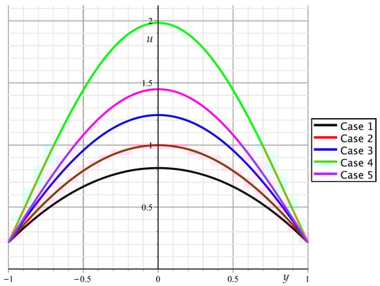
Figure 2.
Velocity profiles for Cases 1–5 with , , , , , , , , , and .
Using the above exact solutions, we have performed an extra verification of the algorithm of constructing weak solutions that was applied by us in Section 5.1 for proving Theorem 1(a). As expected, we have obtained a good agreement between the exact solutions and the suitable Galerkin approximate solutions. This is well illustrated by Figure 3. In the corresponding numerical experiment, the relative percentage error of calculation of the velocity field, constructed by Galerkin’s method with the six basis functions , , …, , is equal to 1.4% with respect to the -norm.
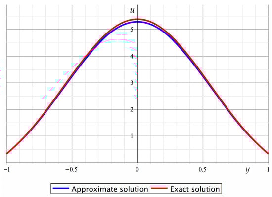
Figure 3.
Velocity profiles for the plane Poiseuille flow with , , , , , , and .
7. Conclusions
In this paper, we have investigated the nonlinear heat and mass transfer model for the unidirectional flow of a viscous fluid through a plane channel under Navier’s slip conditions on the channel walls. The effects of variable viscosity, thermal conductivity, and slip length are taken into account. Using the Galerkin scheme, the generalized Borsuk theorem, and the compactness arguments, we have proved the existence and uniqueness theorems for both weak and strong solutions of the corresponding BVP and derived some properties of solutions. In addition, considering our model subject to some analytical relations for temperature dependence of viscosity, we have obtained the explicit expressions for flow velocity and temperature. The approach proposed in the present work advances the insight of complex heat and mass transfer and is quite universal. This can be applied to studying many other models for temperature-dependent flows of both Newtonian and non-Newtonian fluids in channels and tubes. The authors suggest the following directions for further research:
- well-posedness of initial-boundary value problems for unsteady flows;
- modeling of flows under other kinds of realistic boundary conditions, in particular, under threshold-type slip conditions;
- continuous dependence of solutions on model data;
- stability/instability and limiting behavior of solutions;
- optimization and flow control problems.
Author Contributions
Conceptualization, E.S.B.; methodology, E.S.B. and A.A.D.; investigation, E.S.B. and A.A.D.; writing—original draft preparation, A.A.D.; visualization, A.A.D. and M.A.A.; writing—review and editing, E.S.B., A.A.D. and M.A.A. All authors have read and agreed to the published version of the manuscript.
Funding
This research received no external funding.
Data Availability Statement
Data are contained within the article.
Conflicts of Interest
The authors declare no conflicts of interest.
References
- Baranovskii, E.S. On steady motion of viscoelastic fluid of Oldroyd type. Sb. Math. 2014, 205, 763–776. [Google Scholar] [CrossRef]
- Baranovskii, E.S. Optimal control for steady flows of the Jeffreys fluids with slip boundary condition. J. Appl. Industr. Math. 2014, 8, 168–176. [Google Scholar] [CrossRef]
- Domnich, A.A.; Baranovskii, E.S.; Artemov, M.A. A nonlinear model of the non-isothermal slip flow between two parallel plates. J. Phys. Conf. Ser. 2020, 1479, 012005. [Google Scholar] [CrossRef]
- Whitehead, J.A.; Helfrich, K.R. Instability of flow with temperature-dependent viscosity: A model of magma dynamics. J. Geophys. Res. 1991, 96, 4145–4155. [Google Scholar] [CrossRef]
- Wylie, J.J.; Lister, J.R. The effects of temperature-dependent viscosity on flow in a cooled channel with application to basaltic fissure eruptions. J. Fluid Mech. 1995, 305, 239–261. [Google Scholar] [CrossRef]
- Diniega, S.; Smrekar, S.E.; Anderson, S.; Stofan, E.R. The influence of temperature-dependent viscosity on lava flow dynamics. J. Geophys. Res. 2013, 118, 1516–1532. [Google Scholar] [CrossRef]
- Louis, M.M.; Boyko, E.; Stone, H.A. Effect of temperature-dependent viscosity on pressure drop in axisymmetric channel flows. Phys. Rev. Fluids 2023, 8, 114101. [Google Scholar] [CrossRef]
- Navier, C.L.M.H. Mémoire sur les lois du mouvement des fluides. Mém. Acad. R. Sci. Paris 1822, 6, 389–440. [Google Scholar]
- Ghahramani, N.; Georgiou, G.C.; Mitsoulis, E.; Hatzikiriakos, S.G. J.G. Oldroyd’s early ideas leading to the modern understanding of wall slip. J. Non-Newton. Fluid Mech. 2021, 293, 104566. [Google Scholar] [CrossRef]
- Jäger, W.; Mikelić, A. On the roughness-induced effective boundary conditions for an incompressible viscous flow. J. Differ. Equ. 2001, 170, 96–122. [Google Scholar] [CrossRef]
- Friedmann, E. The optimal shape of riblets in the viscous sublayer. J. Math. Fluid Mech. 2010, 12, 243–265. [Google Scholar] [CrossRef]
- Friedmann, E.; Richter, T. Optimal microstructures drag reducing mechanism of riblets. J. Math. Fluid Mech. 2011, 13, 429–447. [Google Scholar] [CrossRef]
- Achdou, Y.; Pironneau, O.; Valentin, F. Shape control versus boundary control. In Équations aux Dérivées Partielles et Applications: Articles Dédiés à J.L. Lions; Elsevier: Paris, France, 1998; pp. 1–18. [Google Scholar]
- Rajagopal, K.R. On some unresolved issues in non-linear fluid dynamics. Russ. Math. Surv. 2003, 58, 319–330. [Google Scholar] [CrossRef]
- Nahme, R. Beiträge zur hydrodynamischen Theorie der Lagerreibung. Ing. Arch. 1940, 11, 191–209. [Google Scholar] [CrossRef]
- Hagg, A.C. Heat effects in lubricating films. J. Appl. Mech. 1944, 11, A72–A76. [Google Scholar] [CrossRef]
- Bostandzhyan, S.A.; Merzhanov, A.G.; Khudyaev, S.I. Some problems of nonisothermal steady flow of a viscous fluid. J. Appl. Mech. Tech. Phys. 1965, 6, 30–33. [Google Scholar] [CrossRef]
- Ockendon, H.; Ockendon, J.R. Variable-viscosity flows in heated and cooled channels. J. Fluid Mech. 1977, 83, 177–190. [Google Scholar] [CrossRef]
- Zhizhin, G.V. Nonisothermal Couette flow of a non-Newtonian fluid under the action of a pressure gradient. J. Appl. Mech. Tech. Phys. 1981, 22, 306–309. [Google Scholar] [CrossRef]
- Schäfer, P.; Herwig, H. Stability of plane Poiseuille flow with temperature dependent viscosity. Int. J. Heat Mass Transf. 1993, 36, 2441–2448. [Google Scholar] [CrossRef]
- Skulskiy, O.I.; Slavnov, Y.V.; Shakirov, N.V. The hysteresis phenomenon in nonisothermal channel flow of a non-Newtonian liquid. J. Nonnewton. Fluid Mech. 1999, 81, 17–26. [Google Scholar] [CrossRef]
- Ferro, S.; Gnav, G. Effects of temperature-dependent viscosity in channels with porous walls. Phys. Fluids. 2002, 14, 839–849. [Google Scholar] [CrossRef]
- Myers, T.G.; Charpin, J.P.F.; Tshehla, M.S. The flow of a variable viscosity fluid between parallel plates with shear heating. Appl. Math. Model. 2006, 30, 799–815. [Google Scholar] [CrossRef]
- Farooq, M.; Rahim, M.T.; Islam, S.; Siddiqui, A.M. Steady Poiseuille flow and heat transfer of couple stress fluids between two parallel inclined plates with variable viscosity. J. Assoc. Arab Univ. Basic Appl. Sci. 2013, 14, 9–18. [Google Scholar] [CrossRef][Green Version]
- Baranov, A.V. Nonisothermal dissipative flow of viscous liquid in a porous channel. High Temp. 2017, 55, 414–419. [Google Scholar] [CrossRef]
- Ellahi, R.; Zeeshan, A.; Hussain, F.; Abbas, T. Two-phase Couette flow of couple stress fluid with temperature dependent viscosity thermally affected by magnetized moving surface. Symmetry 2019, 11, 647. [Google Scholar] [CrossRef]
- Kudrov, A.I.; Sheremet, M.A. Natural convection of heat-generating liquid of variable viscosity under wall cooling impact. Mathematics 2022, 10, 4501. [Google Scholar] [CrossRef]
- Nizamova, A.D.; Kireev, V.N.; Urmancheev, S.F. Influence of temperature dependence of viscosity on the stability of fluid flow in an annular channel. Lobachevskii J. Math. 2023, 44, 1778–1784. [Google Scholar] [CrossRef]
- Mohanty, R.L.; Mishra, V.K.; Chaudhuri, S. Temperature-dependent viscosity effects on heat transfer characteristics of grade three fluid in electromagnetohydrodynamic flow between large parallel plates maintained at uniform temperatures. Heat Transf. 2024, 53, 3855–3879. [Google Scholar] [CrossRef]
- Tanner, R.I. Engineering Rheology, 2nd ed.; Oxford University Press: Oxford, UK, 2000. [Google Scholar]
- Becker, L.E.; McKinley, G.H. The stability of viscoelastic creeping plane shear flows with viscous heating. J. Nonnewton. Fluid Mech. 2000, 92, 109–133. [Google Scholar] [CrossRef]
- Ghatee, M.H.; Zare, M. Power-law behavior in the viscosity of ionic liquids: Existing a similarity in the power law and a new proposed viscosity equation. Fluid Phase Equilibr. 2011, 311, 76–82. [Google Scholar] [CrossRef]
- Sharma, G.; Hanumagowda, B.N.; Srilatha, P.; Varma, S.V.K.; Khan, U.; Hassan, A.M.; Gamaoun, F.; Kumar, R. Flow and heat transfer analysis of Couette and Poiseuille flow of a hybrid nanofluid with temperature-dependent viscosity and thermal conductivity. Case Stud. Therm. Eng. 2023, 51, 103550. [Google Scholar] [CrossRef]
- Krein, S.G.; Tkhu Kha, C. The problem of the flow of a non-uniformly heated viscous fluid. Comput. Math. Math. Phys. 1989, 29, 127–131. [Google Scholar] [CrossRef]
- Lorca, S.A.; Boldrini, J.L. Stationary solutions for generalized Boussinesq models. J. Differ. Equ. 1996, 124, 389–406. [Google Scholar] [CrossRef]
- Brizitskii, R.V.; Saritskaya, Z.Y. Control problem for generalized Boussinesq model. J. Phys. Conf. Ser. 2019, 1268, 012011. [Google Scholar] [CrossRef]
- Alekseev, G.; Brizitskii, R. Theoretical analysis of boundary value problems for generalized Boussinesq model of mass transfer with variable coefficients. Symmetry 2022, 14, 2580. [Google Scholar] [CrossRef]
- Brizitskii, R.V. Boundary value and control problems for mass transfer equations with variable coefficients. J. Dyn. Control Syst. 2024, 30, 24. [Google Scholar] [CrossRef]
- Boldrini, J.L.; Mallea-Zepeda, E.; Rojas-Medar, M.A. Optimal boundary control for the stationary Boussinesq equations with variable density. Commun. Contemp. Math. 2020, 22, 1950031. [Google Scholar] [CrossRef]
- Brizitskii, R.V.; Saritskaia, Z.Y. Analysis of inhomogeneous boundary value problems for generalized Boussinesq model of mass transfer. J. Dyn. Control Syst. 2023, 29, 1809–1828. [Google Scholar] [CrossRef]
- Alekseev, G.V.; Soboleva, O.V. Solvability analysis for the Boussinesq model of heat transfer under the nonlinear Robin boundary condition for the temperature. Phil. Trans. R. Soc. A 2024, 382, 20230301. [Google Scholar] [CrossRef]
- Andreev, V.K.; Uporova, A.I. Initial boundary value problem on the motion of a viscous heat-conducting liquid in a vertical pipe. J. Sib. Fed. Univ. Math. Phys. 2023, 16, 5–16. [Google Scholar]
- Mallea-Zepeda, E.; Lenes, E.; Valero, E. Boundary control problem for heat convection equations with slip boundary condition. Math. Probl. Eng. 2018, 2018, 7959761. [Google Scholar] [CrossRef]
- Kovtanyuk, A.E.; Chebotarev, A.Y.; Botkin, N.D.; Hoffmann, K.-H. Unique solvability of a steady-state complex heat transfer model. Commun. Nonlinear Sci. Numer. Simul. 2015, 20, 776–784. [Google Scholar] [CrossRef]
- Chebotarev, A.Y.; Pak, N.M.; Kovtanyuk, A.E. Analysis and numerical simulation of the initial-boundary value problem for quasilinear equations of complex heat transfer. J. Appl. Ind. Math. 2023, 17, 698–709. [Google Scholar] [CrossRef]
- Chebotarev, A.Y. Optimal control of quasi-stationary equations of complex heat transfer with reflection and refraction conditions. Comput. Math. Math. Phys. 2023, 63, 2050–2059. [Google Scholar] [CrossRef]
- Chebotarev, A.Y. Inhomogeneous problem for quasi-stationary equations of complex heat transfer with reflection and refraction conditions. Comput. Math. Math. Phys. 2023, 63, 441–449. [Google Scholar] [CrossRef]
- Goruleva, L.S.; Prosviryakov, E.Y. A new class of exact solutions to the Navier–Stokes equations with allowance for internal heat release. Opt. Spectrosc. 2022, 130, 365–370. [Google Scholar] [CrossRef]
- Baranovskii, E.S. Exact solutions for non-isothermal flows of second grade fluid between parallel plates. Nanomaterials 2023, 13, 1409. [Google Scholar] [CrossRef]
- Prosviryakov, E.Y.; Ledyankina, O.A.; Goruleva, L.S. Exact solutions to the Navier–Stokes equations for describing the flow of multicomponent fluids with internal heat generation. Russ. Aeronaut. 2024, 67, 60–69. [Google Scholar] [CrossRef]
- Baranovskii, E.S. The stationary Navier–Stokes–Boussinesq system with a regularized dissipation function. Math. Notes 2024, 115, 670–682. [Google Scholar] [CrossRef]
- Amorim, C.B.; de Almeida, M.F.; Mateus, E. Global existence of solutions for Boussinesq system with energy dissipation. J. Math. Anal. Appl. 2024, 531, 127905. [Google Scholar] [CrossRef]
- Ershkov, S.V.; Christianto, V.; Shamin, R.V.; Giniyatullin, A.R. About analytical ansatz to the solving procedure for Kelvin–Kirchhoff equations. Eur. J. Mech. B/Fluids. 2020, 79, 87–91. [Google Scholar] [CrossRef]
- Fetecau, C.; Bridges, C. Analytical solutions for some unsteady flows of fluids with linear dependence of viscosity on the pressure. Inverse Probl. Sci. Eng. 2021, 29, 378–395. [Google Scholar] [CrossRef]
- Baranovskii, E.S. Feedback optimal control problem for a network model of viscous fluid flows. Math. Notes 2022, 112, 26–39. [Google Scholar] [CrossRef]
- Baranovskii, E.S.; Artemov, M.A. Optimal Dirichlet boundary control for the corotational Oldroyd model. Mathematics 2023, 11, 2719. [Google Scholar] [CrossRef]
- Ershkov, S.V.; Leshchenko, D.D. Non-Newtonian pressure-governed rivulet flows on inclined surface. Mathematics 2024, 12, 779. [Google Scholar] [CrossRef]
- Kim, C.; Pak, J.; Sin, C.; Baranovskii, E.S. Regularity results for 3D shear-thinning fluid flows in terms of the gradient of one velocity component. Z. Angew. Math. Phys. 2024, 75, 69. [Google Scholar] [CrossRef]
- Adams, R.A.; Fournier, J.J.F. Sobolev Spaces, Vol. 40 of Pure and Applied Mathematics; Elsevier: Amsterdam, The Netherlands, 2003. [Google Scholar]
- Baiocchi, C.; Capelo, A. Variational and Quasi Variational Inequalities; J. Wiley and Sons: New York, NY, USA, 1984. [Google Scholar]
- Castillo, R.E.; Rafeiro, H. An Introductory Course in Lebesgue Spaces; Springer Publishing: Cham, Switzerland, 2016. [Google Scholar] [CrossRef]
- Boyer, F.; Fabrie, P. Mathematical Tools for the Study of the Incompressible Navier–Stokes Equations and Related Models; Springer: New York, NY, USA, 2013. [Google Scholar] [CrossRef]
- O’Regan, D.; Cho, Y.J.; Chen, Y.Q. Topological Degree Theory and Applications; Chapman and Hall/CRC: New York, NY, USA, 2006. [Google Scholar] [CrossRef]
- Dinca, G.; Mawhin, J. Brouwer Degree: The Core of Nonlinear Analysis; Birkhäuser: Cham, Switzerland, 2021. [Google Scholar] [CrossRef]


Disclaimer/Publisher’s Note: The statements, opinions and data contained in all publications are solely those of the individual author(s) and contributor(s) and not of MDPI and/or the editor(s). MDPI and/or the editor(s) disclaim responsibility for any injury to people or property resulting from any ideas, methods, instructions or products referred to in the content. |
© 2024 by the authors. Licensee MDPI, Basel, Switzerland. This article is an open access article distributed under the terms and conditions of the Creative Commons Attribution (CC BY) license (https://creativecommons.org/licenses/by/4.0/).