Abstract
This paper addresses the valuation of European options, which involves the complex and unpredictable dynamics of fractal market fluctuations. These are modeled using the -order time-fractional Black–Scholes equation, where the Caputo fractional derivative is applied with the parameter ranging from 0 to 1. We introduce a novel, high-order numerical scheme specifically crafted to efficiently tackle the time-fractional Black–Scholes equation. The spatial discretization is handled by a tailored finite point scheme that leverages exponential basis functions, complemented by an L1-discretization technique for temporal progression. We have conducted a thorough investigation into the stability and convergence of our approach, confirming its unconditional stability and fourth-order spatial accuracy, along with -order temporal accuracy. To substantiate our theoretical results and showcase the precision of our method, we present numerical examples that include solutions with known exact values. We then apply our methodology to price three types of European options within the framework of the time-fractional Black–Scholes model: (i) a European double barrier knock-out call option; (ii) a standard European call option; and (iii) a European put option. These case studies not only enhance our comprehension of the fractional derivative’s order on option pricing but also stimulate discussion on how different model parameters affect option values within the fractional framework.
Keywords:
time-fractional Black–Scholes equation; tailored finite point scheme; L1 discretization formula; exponential functions; European option pricing MSC:
35Q91; 45K05; 65M06; 91B02
1. Introduction
Options rank as some of the most frequently traded financial instruments globally. The precise valuation of these instruments has been a central theme in financial research since the seminal Black–Scholes (B-S) model was formulated by Black, Scholes [1] and Merton [2] in 1973. Although the B-S model is foundational in financial theory and has been instrumental in valuing a variety of equity options, including European and American styles, and in creating portfolios that replicate option values, it has notable limitations. It struggles to accommodate rapid market fluctuations and price jumps that happen within brief periods [3].
Fractional calculus has gained prominence in stochastic modeling and financial economics since it was recognized that asset price dynamics often exhibit fractal properties. Pioneering works such as Wyss’s [4] fractional adaptation of a time-fractional B-S model for pricing European call options highlighted the potential of fractional derivatives to better reflect real-world market behavior. More recently, there has been a burgeoning interest in applying fractional derivatives and integrals due to their exceptional capability in accounting for past influences through their non-local attributes [5]. In [6], Jumarie derived the time and space fractional B-S models for stock exchange dynamics and gave an optimal fractional Merton’s portfolio. Liang et al. [7] advanced the field by deriving both single and bi-parameter fractional Black–Scholes–Merton differential equations, assuming that the stock price evolution adheres to a fractional Ito process. In this study, we focus specifically on the time-fractional adaptation of the B-S model
subject to the constraints of the boundary conditions and the terminal state requirement
Here, S denotes the stock’s current price, represents the present time, and signifies the value of a European option price, which depends on S and . The term T refers to the expiration date of the contract, stands for the risk-free interest rate, and represents the volatility inherent in the returns of the underlying asset. Further, is the modified Reimann–Liouville derivative defined as
Setting in (1) and (2), we derive
with boundary and initial conditions
Denoting , the system (4) and (5) can be simplified to
Furthermore, the fractional derivative employed in Equation (6) is specifically the Caputo fractional derivative. This type of derivative is commonly used when dealing with initial value problems involving fractional order differential equations, as it allows for classical initial conditions to be imposed. The Caputo derivative is defined as
Analytical solutions for fractional differential equations are often elusive, prompting researchers to obtain solutions via approximation methods when tackling the time-fractional B-S model. For instance, Zhang et al. [8] proposed a second-order accurate finite difference method coupled with a fast bi-conjugate gradient-stabilized algorithm to minimize storage requirements and numerically solve a time-fractional B-S model. Tian et al. [9] presented three compact difference schemes tailored to the time-fractional B-S model for European option pricing. They employed an exponential transformation to eliminate the convection term in the B-S equation and achieved fourth-order spatial accuracy via the Padé approximation.
Samuel et al. [10] put forth a robust numerical method grounded in the extension of the Crank–Nicolson finite difference approach for solving the time-fractional B-S model characterizing stock market dynamics. Roul et al. [11] developed a fourth-order compact finite difference method utilizing quintic B-spline basis functions, while Abdi et al. [12] constructed high-order accurate compact difference schemes in space. Golbabai et al. [13,14] presented the utilization of radial basis functions within a meshless framework for numerically addressing the time-fractional B-S equation. Their work revealed a convergence rate of in relation to the time variable.
Akram et al. [15] utilized the extended cubic B-spline to generalize the collocation method for the time-fractional B-S European option pricing model. Their approach’s distinctive characteristic lies in transforming such problems into systems of algebraic equations suitable for computer implementation, with a spatial convergence rate of 2. A distinct space-time spectral approach was introduced, employing Jacobi polynomials for temporal discretization and Fourier-type basis functions for spatial discretization [16]. Zhang et al. [17] derived a numerical scheme with second-order spatial accuracy, which was subsequently enhanced by De Staelen et al. [18] through the development of a fourth-order spatially accurate scheme.
Fractional calculus, with its non-local properties, is essential for modeling memory effects and has led to the development of efficient numerical methods for solving fractional differential equations [19,20,21,22].These methods include finite difference [23], finite element [24], finite volume [25], spectral [26,27], local discontinuous Galerkin finite elements [28], and meshless methods [29]. Recently, we have focused on tailored finite point schemes (TFPSs) for solving a variety of fractional diffusion equations, including those that describe convection-dominated diffusion and anisotropic subdiffusion [30,31]. TFPS, first introduced by Han et al. [32] for singularly perturbed elliptic equations and later extended to other models [33,34], uses local basis functions that satisfy the homogeneous equation with constant coefficients. This approach allows for remarkable accuracy even at coarser grid resolutions by closely matching the intrinsic properties of the solution. TFPS has proven effective in capturing boundary and interface layers within fractional diffusion problems, prompting its application in our study to formulate a TFPS approach for the time-fractional Black–Scholes Model.
In this paper, we introduce a novel high-order tailored finite TFPS specifically crafted for solving the time-fractional Black–Scholes equation with high accuracy. Our approach differs from the compact finite difference methods referenced in [11,12,35], which rely on high-order Taylor series expansions, by starting with the exact solution of the local grid cell equation and constructing linear relationships among nodes based on their positional arrangements. This method inherently aligns with the exact solution, enabling the development of a finite difference scheme with high-order accuracy. We introduce two key innovations: first, the development of a TFPS that uses exponential basis functions for spatial discretization and an L1-discretization for time-stepping, which we have shown to be unconditionally stable with fourth-order spatial accuracy and -order temporal accuracy through a thorough analysis; and second, an in-depth exploration of the impact of the fractional derivative order on option pricing, along with a discussion on the influence of different model parameters on option prices within the context of this model.
The structure of this paper is outlined as follows: Section 2 presents our TFPS, which achieves fourth-order accuracy in spatial discretization for the time-fractional B-S model. Section 3 delves deeply into the theoretical aspects, analyzing the stability and convergence of the proposed method. Section 4 presents a comprehensive set of numerical experiments, offering empirical evidence that demonstrates the efficiency and reliability of our method. This paper closes with a summary in Section 5.
2. TFPS for a Time-Fractional B-S Model
For the numerical resolution of model (6), we restrict the unbounded domain of the variable x to a finite interval and, without loss of generality, introduce a source term on the right-hand side of the equation. Consequently, we obtain
2.1. The Main Idea of TFPS for Convection–Diffusion Equations
Our starting point consists of the convection–diffusion equations in their steady-state configuration, which can be expressed as follows:
Suppose the computational domain is . Let , with . On , , Equation (8) can be approximated by
where is an approximation to .
The framework of the TFPS
Let
Then, w satisfies
In the subsequent part, we construct a discretization scheme for (11), and then we can obtain the TFPS for (9).
Step one: To build finite difference scheme for (11). Similarly to what has been carried out in [33,34], the exact solution of (11) can be expressed as the special form ; then, is the solution to
We can obtain . The general solutions of (11) belong to the linear space
The TFPS aims at devising a discrete representation of the variable w, structured as follows:
To accurately deduce the coefficients , , we employ the two basis functions , , which are specifically chosen to fulfill Equation (14) precisely. A simple calculation gives
For any nonzero constant , ref. (15) has the unique solution
Thus, the discretized scheme derived from (11) can be formulated as
Step two: To build TFPS for (9).
Substituting Equation (10) into Equation (17) results in the following expression
By replacing with , we can obtain the TFPS for (9)
Applying expansion methods where exponentials are expanded in terms of their argument, we obtain a modified differential equation that corresponds to the aforementioned finite difference scheme and is given as
where
indicating that the accuracy of this scheme is of the second order.
2.2. Fourth-Order TFPS for Convection–Diffusion Equations
The scheme (19) clearly exhibits diagonal dominance. As the most straightforward instance within the TFPS, this -accurate scheme serves as our foundation. Our objective is to make subtle refinements to the core Formula (19) in order to enhance its accuracy to the fourth order. Considering that Formula (20) deviates from the baseline Equation (9) by a mere second-order small quantity, we propose that the fourth-order formulation maintains the same structure as scheme (19), with the sole distinction being the inclusion of second-order corrections to the convective coefficient and the source term. We have
where
Define the modified coefficient . This is used in an equivalent discrete differential equation
It can be seen that an accuracy is achieved if only
From (20), we have
By substituting the system represented by Equation (25) into Equation (23), we derive expressions for the perturbation values
2.3. Temporal Discretization
Now, we proceed to address the numerical resolution of the time-fractional problem presented in system (7). To accomplish this, our initial step involves transforming (7) into the form of (8). The equivalent formulation for (7) reads as follows:
Let , and replace g in (29) by , then we can adopt the scheme to give the approximation scheme for (29). Given a grid , , with , and N is a positive integer. The values of at grid point are denoted by . Therefore, we obtain
The Caputo fractional time derivative present in (30) is approximated via the L1 scheme,
Lemma 1
([21,26]). Suppose . Let
then
where and .
Lemma 2
Lemma 3.
Let , ; then, we have
Proof.
Assuming the function is defined as , ; through the application of the Mean Value Theorem for differentiation, we deduce that
Thus
□
2.4. Fourth Order TFPS for the Time-Fractional Black–Scholes Model
Denote , . At this stage, we are equipped to outline the implicit version of the TFPS approach to (7). is the numerical solution of , omitting the truncation errors in (30). To begin with, we proceed by solving for the numerical solutions through the following steps:
Then, the numerical solutions are computed via the following procedure
with the initial and boundary conditions
Proof.
As the TFPS scheme embodied by Equations (36) and (37) constitutes a linear method, it is necessary to verify that its coefficient matrix exhibits diagonal dominance as . Given that the functions , , are all continuous, and considering , the distinction between subscripts (, i or ) can be disregarded for our purposes. Let us assume that . By applying Taylor expansions to the exponential functions , , we obtain the following insights:
Then
Consequently, due to the strict diagonal dominance of the coefficient matrix A, we can confirm the existence and uniqueness of the solution in the fourth-order TFPS. □
Remark 1.
The TFPS (36) and (37) maintains the three-point stencil and ensures the strict diagonal dominance of the coefficient matrix A. To solve the linear equations associated with a tridiagonal matrix, several rapid computational methods can be utilized. Among these, the Thomas algorithm is a direct and efficient method for solving tridiagonal systems.
3. Theoretical Analysis of the Fourth-Order TFPS
3.1. The Local Truncation Error
Denote
Utilizing Taylor series expansions, we can demonstrate that for the genuine solution of the system comprised of system (36) and (37), which is assumed to be sufficiently smooth, the following relationship holds true:
Applying Lemma 1, we obtain the following result:
Thus, the local truncation error for the TFPS scheme defined by systems (36) and (37) is estimated to be
This estimation is valid across the indices and .
3.2. Stability Analysis for Constant Coefficients
In this section, we examine the stability of the TFPS through a Fourier analysis approach. Initially, we introduce a lemma that will play a crucial role in our subsequent discussion.
Lemma 4
(Discrete Gronwall’s inequality [19]). Assume that y is a non-negative constant and and sequences. If the inequality
holds, then it follows that
For the current stability analysis based on the Fourier method, we restrict ourselves to equations with constant coefficients. Considering that B, and r are all constants at this point, we remove their indices n in the coefficient. Let denote the solution of (36) and (37) with an initial condition . Define the perturbation term as
then, we have
We interpolate from the discrete mesh point onto the control volume (, using piecewise constant functions, thereby yielding a continuous function defined over the interval . Since we are dealing with Dirichlet boundary conditions, we have at the boundaries; hence, we can extend it periodically throughout the entire domain. Consequently, the Fourier series representation of is given by
This series allows us to express the perturbation function in terms of its frequency components across the periodic domain. For any vector , we define the discrete norm as , and with this,
Lemma 5.
The discrete Fourier coefficients are
Furthermore, we can apply the discrete version of Parseval’s identity for the Fourier transform, which states that
In order to investigate the stability of our scheme relative to initial perturbations, we may introduce the simplifying expression , where , and subsequently substitute this into Equation (39). This leads us to derive
To establish the unconditional stability of the scheme under any initial conditions, we must initially validate the subsequent lemma.
Lemma 6.
Let it be assumed that is determined by the relation (40). Then, for any , the following inequality holds
Proof.
We shall substantiate that using mathematical induction. With reference to (41), we aim to demonstrate the validity of the following inequality:
Denote , = , = , . Assume that the inequality we are referring to is given by (42), which takes the form
and note that . To prove (43), it is sufficient that we prove that
As (44) is equivalent to
Note that
and
The given inequality
naturally holds true as . This, in turn, ensures the validity of (44). As a result, (42) is also proven true. It is easy to see that . Assume that holds for ; then using (41) and Lemma 2, we can derive
and the mathematical induction is completed. □
Proof.
Using Lemma 6, we obtain
and the proof is finished. □
3.3. Convergence Analysis of TFPS
In this section, we delve into the investigation of the convergence properties of the TFPS. Let be defined as
By substituting Equation (45) in Equation (37), and noticing that , we have
where . In line with the analogous reasoning employed in the stability analysis, we proceed to express both and in terms of their corresponding Fourier series expansions as follows:
Employing Parseval’s equality in conjunction with the definition of the norm, we arrive at
where
Now, assume that
where . Inserting the expressions from Equation (49) into Equation (46), followed by a series of simplifications, we obtain
Lemma 7.
Let represent the solution corresponding to Equation (50). Consequently, there exists a positive constant K, such that
Proof.
Theorem 3.
The TFPS is convergent in the norm, and the order of convergence is .
Proof.
Utilizing Lemma 7 alongside the expressions from Equation (48), we obtain the following
This completes the proof. □
4. Numerical Example
In this section, we showcase the accuracy and convergence rate of TFPS introduced in Section 2 through two test cases featuring known exact solutions. Additionally, we deploy this scheme to compute the prices of various European options under the auspices of a time-fractional B-S model, which constitutes a particularly significant and intriguing model within financial markets. To test the order of convergence for the norm, we progressively refine the mesh by halving both the spatial step size h to and the time step size to . The number of time steps N is then determined by rounding the quantity to the nearest integer.
Example 1.
Consider the following time-fractional B-S model subject to homogeneous boundary conditions
where the source term
is chosen so that the exact solution of (52) is . Here we take the parameter values as .
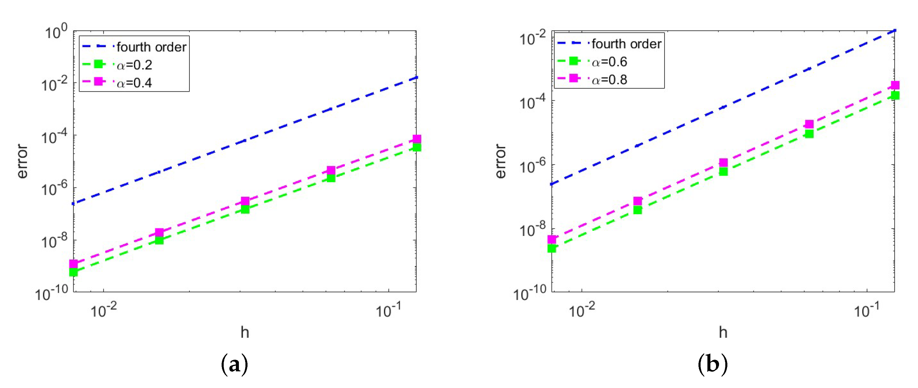
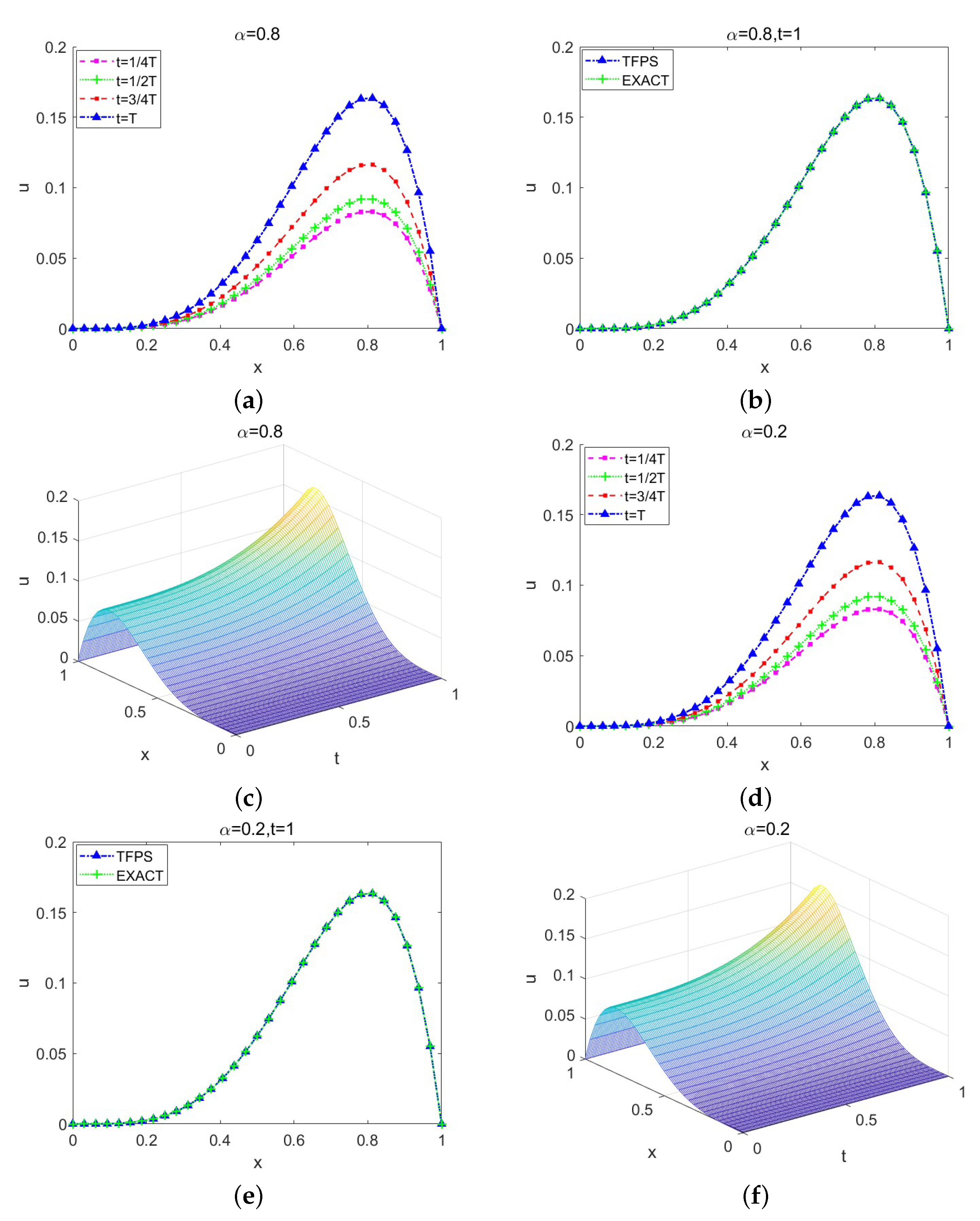
Table 1 presents the errors in the norm for varying fractional order . The corresponding convergence rates are displayed in Figure 1. The observed convergence rates of the TFPS corroborate the findings put forth by Theorem 3. The numerical solutions produced by the TFPS exhibit striking agreement with the corresponding exact solutions as depicted in Figure 2.

Table 1.
The errors of TFPS for different .
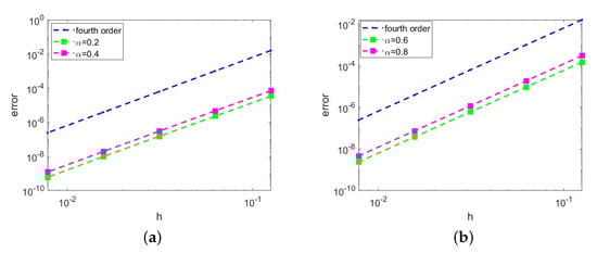
Figure 1.
The convergence order of the norm. (a) . (b) .
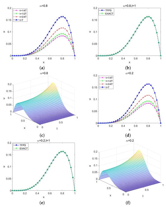
Figure 2.
TFPS for . (a) , for . (b) , and at t = 1. (c) , . (d) , for . (e) , and at . (f) , .
Example 2.
Consider the following time-fractional B-S model subject to homogeneous boundary conditions
The exact solution of (53) is chosen as , the source term is defined as
Here, the parameters’ values are .
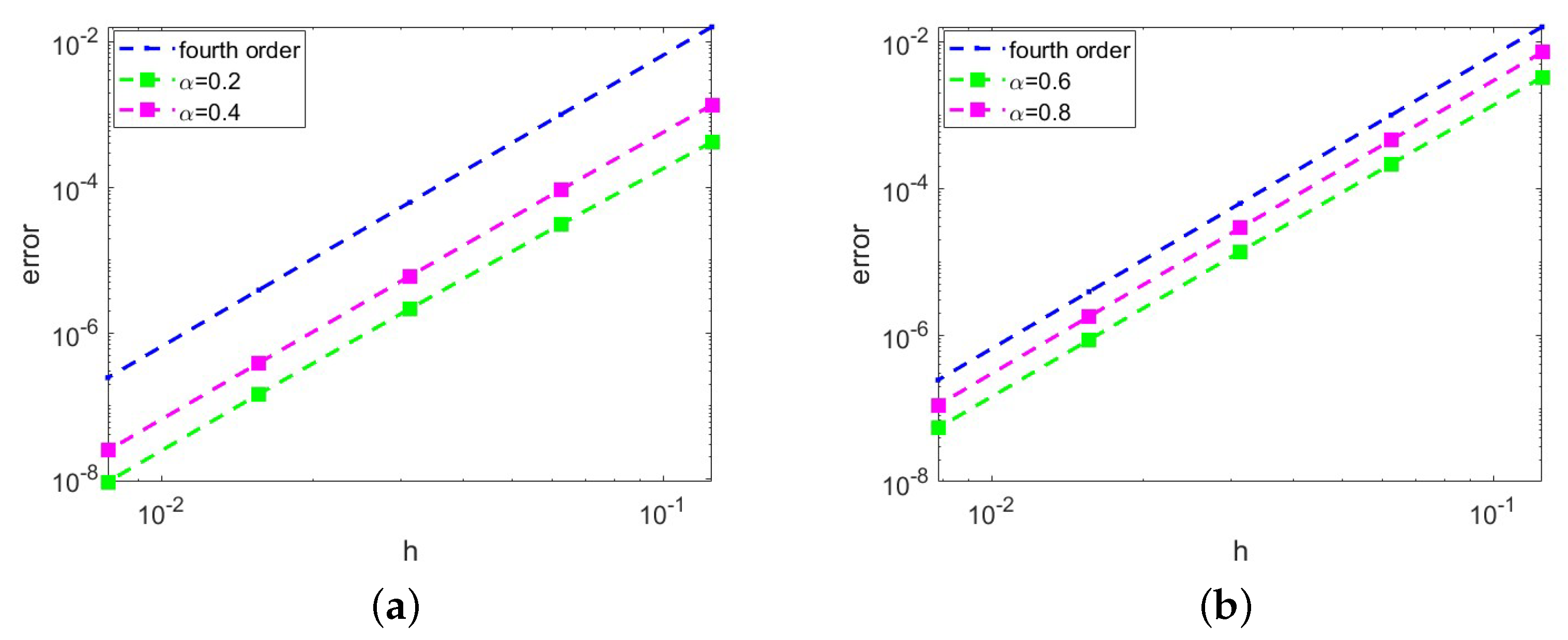
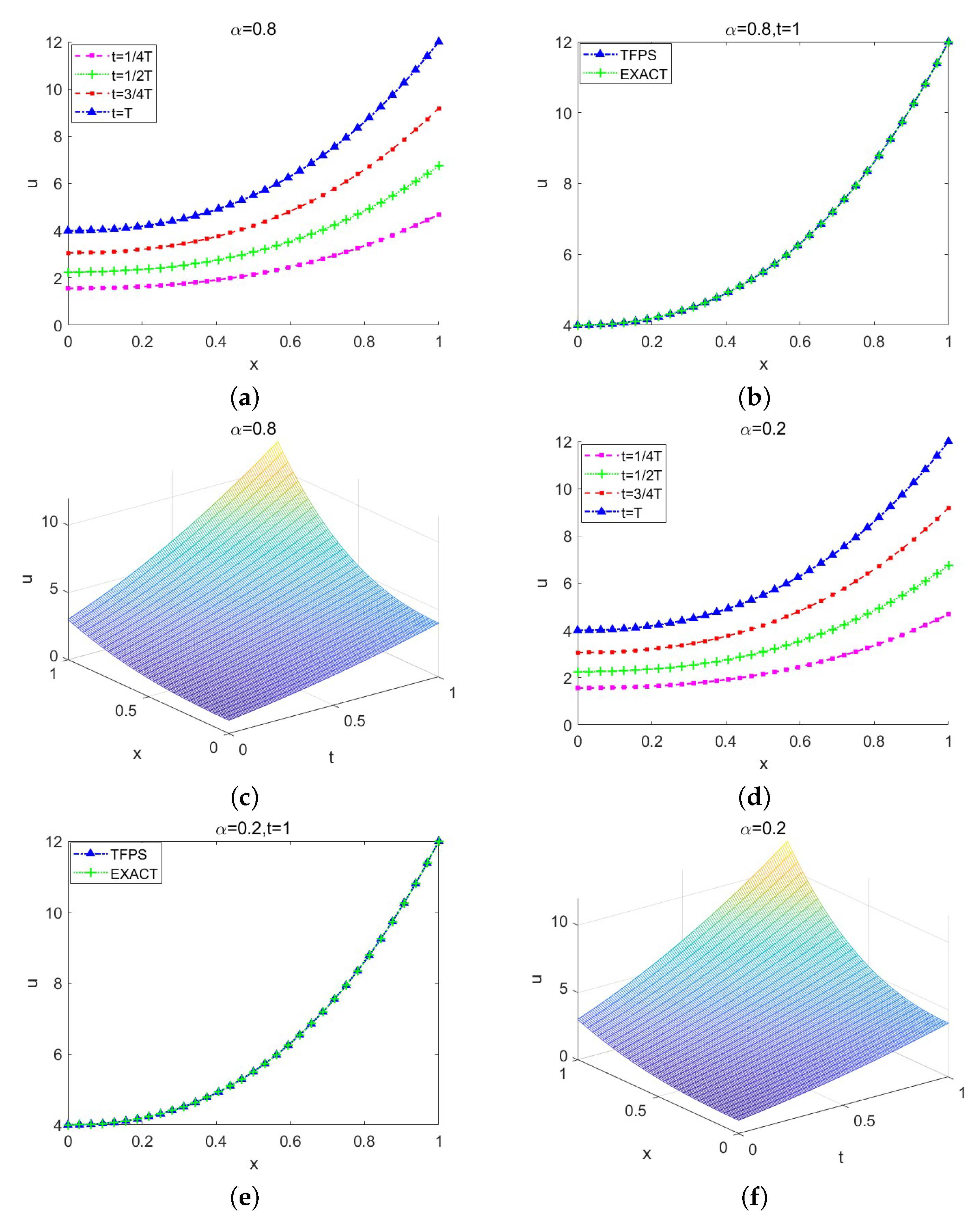
Table 2 presents norm errors for different fractional orders , while Figure 3 showcases the corresponding convergence rates. These convergence rates obtained with the TFPS align consistently with the theoretical predictions established by Theorem 3. The observed convergence rates of the TFPS corroborate the findings put forth by Theorem 3. The excellent correspondence between the numerical solutions generated by the TFPS and the exact solutions is visually demonstrated in Figure 4.
Table 2.
The errors of TFPS for different values.
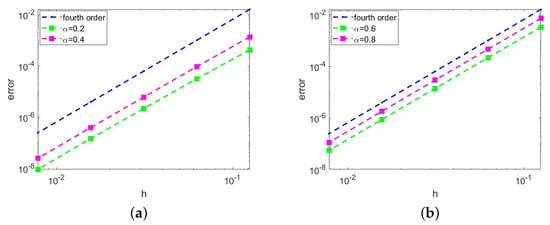
Figure 3.
The convergence order of the norm. (a) . (b) .
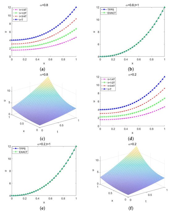
Figure 4.
TFPS for . (a) , for . (b) , and at t = 1. (c) , . (d) , for . (e) , and at t = 1. (f) , .
Example 3.
In this example, we implement the TFPS to calculate the prices of several distinct European options within the framework of a time-fractional B-S model.
Case 1: In the scenario where the payoff function is given by and , the model (55) describes a time-fractional B-S model for pricing a European double barrier knock-out call option. The option price curves for varying are depicted in Figure 5a, with parameters (year), and the dividend yield . The parameters values are selected according to the paper [12,17]. The attributes of Figure 5 are similar to those described in [12,17] perfectly. Observing Figure 5a, we notice that the time-fractional B-S model generates lower option prices when S is beneath a critical threshold near the strike price K, thereby illustrating the presence of fat tails. Conversely, the model provides higher prices for in-the-money options . Thus, compared to the standard B-S process, the time-fractional B-S Model more accurately captures the essence of sudden jumps or substantial movements in asset prices. The option price curves for varying at are depicted in Figure 5b. The model generates lower options prices when but provides higher options prices when at smaller .
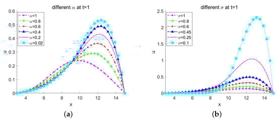
Figure 5.
Double barrier option prices obtained by TFPS. (a) Different at . (b) Different at .
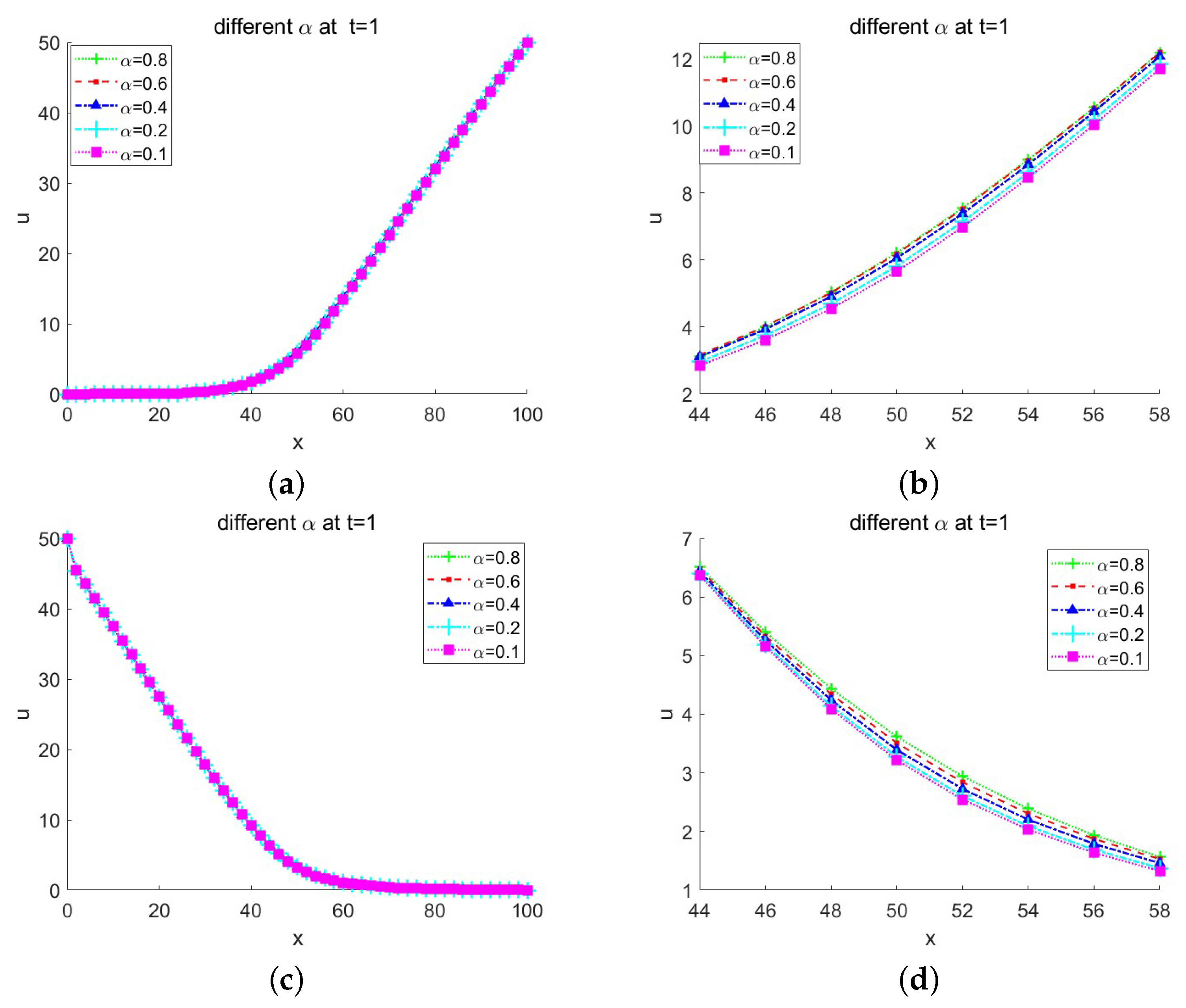
Case 2: For the European call option, the initial and boundary conditions are set as and . The corresponding call option price curves for different values at are illustrated in Figure 6a,b, with the parameters specified as and (year).
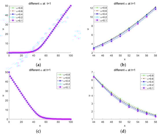
Figure 6.
(a,b) call option prices for different values. (c,d) put option prices for different values.
Case 3: In parallel, the European put option is characterized by the conditions and . The associated put option price curves for different at are plotted in Figure 6c,d, again with the parameters and (year).
Applying the TFPS, the numerical solution of case 2 and case 3 for different values of parameters are plotted in Figure 6, Figure 7 and Figure 8. The following points summarize the findings from the numerical solutions of call and put option prices under various conditions:
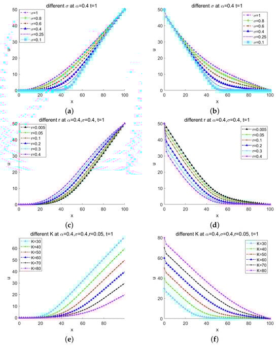
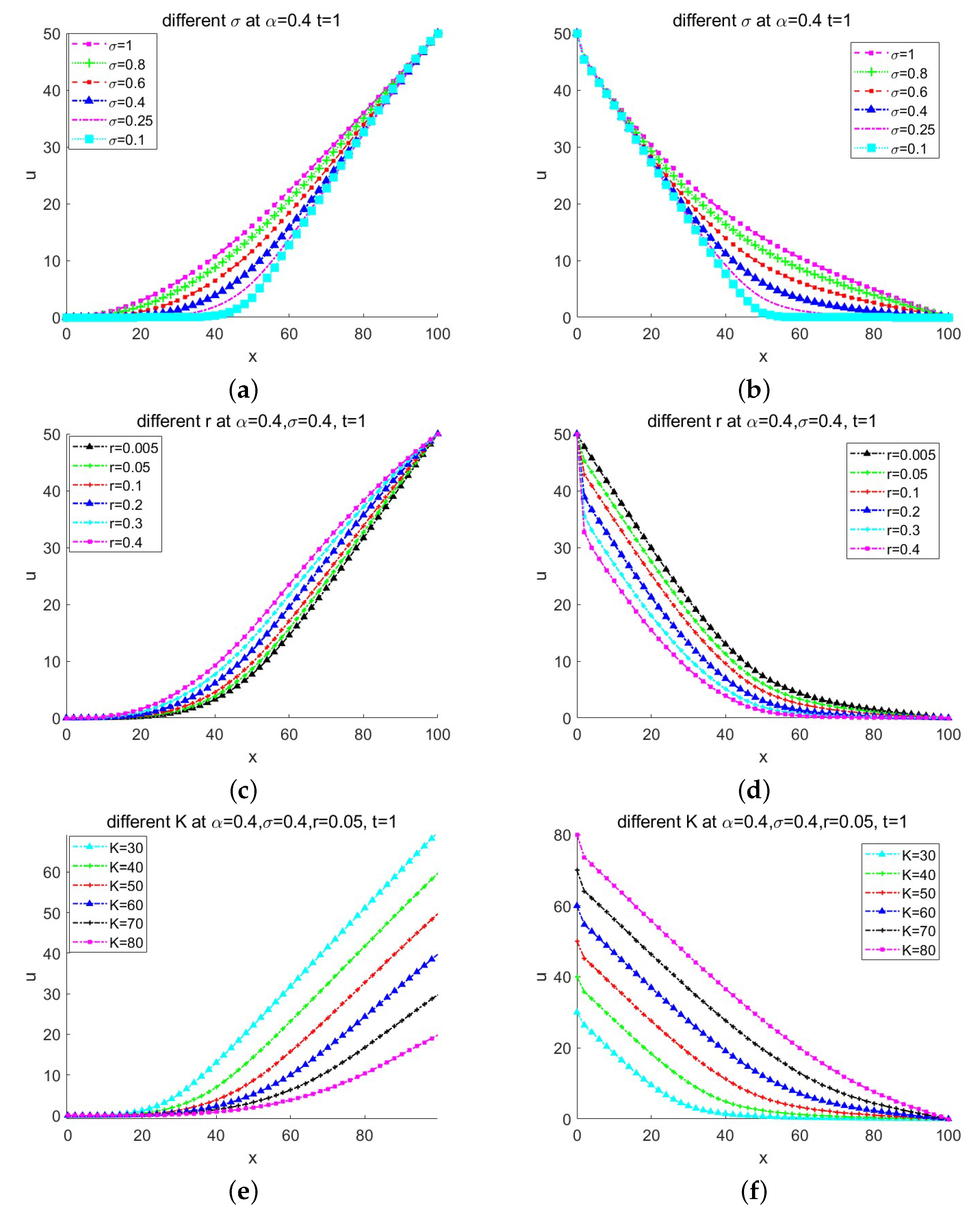
Figure 7.
(a) call option price with different values. (b) put option price with different values. (c) call option price with different r values. (d) put option price with different r values; (e) call option price with different K values. (f) put option price with different K values.
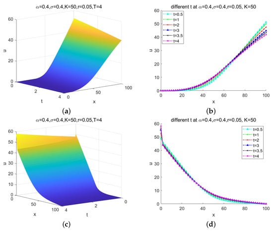
Figure 8.
(a,b) the numerical solution of the TFPS for call option prices in . (c,d) the numerical solution of the TFPS for put option prices in .
- Impact of Time-Fractional Derivatives: The numerical solution of the call option and put option price for varying are depicted in Figure 6. Figure 6 illustrates how time-fractional derivatives notably affect option prices, particularly around the at-the-money region . However, their impact diminishes for options that are either deeply out-of-the-money or deeply in-the-money.
- Volatility Influence: The effect of the stock price’s volatility on option prices when , and for different is shown in Figure 7a,b. Reflecting real-world dynamics, higher volatility leads to higher potential gains, as evidenced by the larger option prices when the stock price is close to the exercise price.
- Risk-Free Interest Rates: The role of risk-free interest rates on option pricing with , , , and across different values of r (0.005, 0.05, 0.1, 0.2, 0.3, 0.4) is portrayed in Figure 7c,d. These figures indicate that higher interest rates tend to increase call option prices while decreasing put option prices.
- Strike Price Effect: The change in option price due to the strike price is presented in Figure 7e,f. This illustrates that higher strike prices result in lower call option values, whereas increasing strike prices lead to escalating put option prices.
- Expiration Date Impact:Figure 8 explores how the expiration date influences call and put option prices. When the stock price significantly exceeds the strike price, a call option featuring a shorter expiration period assumes greater value compared to an option with a longer tenure; conversely, a put option endowed with a longer expiration horizon is more beneficial. In instances where the stock price significantly undershoots the strike, a call option possessing a longer expiration and a put option with a shorter expiry prove more favorable.
All these empirical outcomes align with actual market behaviors, providing a strong basis for understanding and predicting option pricing dynamics in real-world financial markets.
5. Conclusions
In this study, we developed a TFPS for solving the time-fractional B-S model pertinent to European option pricing. The temporal variable was discretized via the L1 scheme, while the spatial variable was treated using the TFPS approach. The stability and convergence properties of the TFPS were thoroughly examined. Theoretical results established the stability of the proposed TFPS method. Furthermore, we demonstrated that the method exhibits -order accuracy with respect to the time dimension and fourth-order accuracy in the spatial domain.
Numerical experiments were performed to validate the effectiveness and accuracy of the novel technique. The results unequivocally demonstrated that our proposed numerical method excels in precisely pricing European options, with convergence rates aligning with theoretical expectations. As a practical demonstration, we applied our methodology to price three distinct categories of European options under the time-fractional Black–Scholes (B-S) model.
Given that the financial payoff function for options at the strike price is frequently nonsmooth, the Temporal Fractional Partial Differential Equation Solver (TFPS) may not attain the desired fourth-order spatial convergence. To mitigate this numerical limitation, we can employ piecewise uniform meshes and/or local mesh refinement techniques without compromising the efficiency of our rapid temporal discretization method. Addressing this challenge will be a key focus of our future research. Looking ahead, we anticipate extending the higher-order TFPS and parallel-in-time method [36] to multidimensional B-S models in the coming future.
Author Contributions
Conceptualization, Y.W.; methodology, Y.W.; software, X.C.; validation, Y.W.; investigation, X.C. and Y.W.; writing—original draft, X.C. and Y.W. All authors have read and agreed to the published version of the manuscript.
Funding
This research was funded by the National Natural Science Foundation of China (Grant Numbers 11901393).
Data Availability Statement
No new data were created or analyzed in this study. Data sharing is not applicable to this article.
Acknowledgments
Thank you to the anonymous reviewer for their constructive suggestions, which have significantly contributed to improving the quality of the article.
Conflicts of Interest
The authors declare no conflicts of interest.
References
- Black, F.; Scholes, M. The pricing of options and corporate liabilities. J. Political Econ. 1973, 81, 637–654. [Google Scholar] [CrossRef]
- Merton, R.C. Theory of rational option pricing. Bell J. Econ. Manag. Sci. 1973, 4, 141–183. [Google Scholar] [CrossRef]
- Carr, P.; Wu, L. The finite moment log stable process and option pricing. J. Financ. 2003, 58, 753–777. [Google Scholar] [CrossRef]
- Wyss, W. The fractional Black–Scholes equation. Fract. Calc. Appl. Anal. 2000, 3, 51–61. [Google Scholar]
- Podlubny, I. Fractional Differential Equations; Academic Press: San Diego, CA, USA, 1999. [Google Scholar]
- Jumarie, G. Stock exchange fractional dynamics defined as fractional exponential growth driven by (usual) gaussian white noise. Application to fractional Black–Scholes equations. Insur. Math. Econ. 2008, 42, 271–287. [Google Scholar] [CrossRef]
- Liang, J.R.; Wang, J.; Zhang, W.J.; Qiu, W.Y.; Ren, F.Y. Option pricing of a bi-fractional Black-Merton-Scholes model with the hurst exponent h in [12, 1]. Appl. Math. Lett. 2010, 23, 859–863. [Google Scholar] [CrossRef]
- Zhang, H.; Liu, F.; Turner, I.; Chen, S. The numerical simulation of the tempered fractional Black–Scholes equation for european double barrier option. Appl. Math. Model. 2016, 40, 5819–5834. [Google Scholar] [CrossRef]
- Tian, Z.W.; Zhai, S.Y.; Weng, Z.F. Compact finite difference schemes of the time-fractional Black–Scholes model. J. Appl. Anal. Comput. 2020, 10, 904–919. [Google Scholar] [CrossRef]
- Nuugulu, S.M.; Gideon, F.; Patidar, K.C. A robust numerical scheme for a time-fractional Black–Scholes partial differential equation describing stock exchange dynamics. Chaos Solitons Fractals 2021, 145, 110753. [Google Scholar] [CrossRef]
- Roul, P.; Goura, V.M.K.P. A compact finite difference scheme for fractional Black–Scholes option pricing model. Appl. Numer. Math. 2021, 166, 40–60. [Google Scholar] [CrossRef]
- Abdi, N.; Aminikhah, H.; Sheikhani, A.H.R. High-order compact finite difference schemes for the time-fractional Black–Scholes model governing European options. Chaos Solitons Fractals 2022, 162, 112423. [Google Scholar] [CrossRef]
- Golbabai, A.; Nikan, O.; Nikazad, T. Numerical analysis of time-fractional Black–Scholes european option pricing model arising in financial market. Comput. Appl. Math. 2019, 38, 173. [Google Scholar] [CrossRef]
- Golbabai, A.; Nikan, O. A computational method based on the moving least-squares approach for pricing double barrier options in a time-fractional Black–Scholes model. Comput. Econ. 2020, 55, 119–141. [Google Scholar] [CrossRef]
- Akram, T.; Abbas, M.; Abualnaja, K.; Iqbal, A.; Majeed, A. An efficient numerical technique based on the extended cubic B-spline functions for solving time fractional Black–Scholes model. Eng. Comput. 2021, 12, 1–12. [Google Scholar] [CrossRef]
- An, X.; Liu, F.; Zheng, M.; Anh, V.; Turner, I. A space-time spectral method for time-fractional Black-Bcholes equation. Appl. Numer. Math. 2021, 165, 152–166. [Google Scholar] [CrossRef]
- Zhang, H.; Liu, F.; Turner, I.; Yang, Q. Numerical solution of the time-fractional Black–Scholes model governing european options. Comput. Math. Appl. 2016, 71, 1772–1783. [Google Scholar] [CrossRef]
- Staelen, R.H.D.; Hendy, A.S. Numerically pricing double barrier options in a time-fractional Black–Scholes model. Comput. Math. Appl. 2017, 74, 1166–1175. [Google Scholar] [CrossRef]
- Li, C.P.; Cai, M. Theory and Numerical Approximations of Fractional Integrals and Derivatives; SIAM: Philadelphia, PA, USA, 2019. [Google Scholar]
- Li, C.P.; Wang, Z. Numerical methods for the time-fractional convection-diffusion-reaction equation. Numer. Funct. Anal. Optim. 2021, 42, 1115–1153. [Google Scholar] [CrossRef]
- Yang, Z.; Zeng, F. A Corrected L1 Method for a Time-Fractional Subdiffusion Equation. J. Sci. Comput. 2023, 95, 85. [Google Scholar] [CrossRef]
- Yang, Z.; Zeng, F. A linearly stabilized convolution quadrature method for the time-fractional Allen-Cahn equation. Appl. Math. Lett. 2023, 144, 108698. [Google Scholar] [CrossRef]
- Roul, P.; Goura, V.M.K.P. A sixth order numerical method and its convergence for generalized Black–Scholes PDE. J. Comput. Appl. Math. 2020, 377, 112881. [Google Scholar] [CrossRef]
- Jin, B.; Lazarovb, R.; Liu, Y.; Zhou, Z. The galerkin finite element method for a multi-term time-fractional diffusion equation. J. Comput. Phys. 2015, 281, 825–843. [Google Scholar] [CrossRef]
- Wang, H.; Cheng, A.; Wang, K. Fast finite volume methods for space-fractional diffusion equations. Discret. Contin. Dyn. Syst. Ser. B 2015, 20, 1427–1441. [Google Scholar] [CrossRef]
- Lin, Y.M.; Xu, C.J. Finite difference/spectral approximations for the time-fractional diffusion equation. J. Comput. Phys. 2007, 225, 1533–1552. [Google Scholar] [CrossRef]
- Taghipour, M.; Aminikhah, H. A spectral collocation method based on fractional Pell functions for solving time–fractional Black–Scholes option pricing model. Chaos Solitons Fractals 2022, 163, 112571. [Google Scholar] [CrossRef]
- Li, C.P.; Wang, Z. The local discontinuous galerkin finite element methods for caputo-type partial differential equations: Mathematical analysis. Appl. Numer. Math. 2020, 150, 587–606. [Google Scholar] [CrossRef]
- Gu, Y.; Sun, H.G. A meshless method for solving three-dimensional time-fractional diffusion equation with variable-order derivatives. Appl. Math. Model. 2020, 78, 539–549. [Google Scholar] [CrossRef]
- Wang, Y.H.; Cao, J.X.; Fu, J. Tailored finite point method for time-fractional convection dominated diffusion problems with boundary layers. Math. Methods Appl. Sci. 2020, 47, 11044–11061. [Google Scholar] [CrossRef]
- Wang, H.; Cao, J.X. A tailored finite point method for subdiffusion equation with anisotropic and discontinuous diffusivity. Appl. Math. Comput. 2021, 401, 125907. [Google Scholar] [CrossRef]
- Han, H.; Huang, Z.Y.; Kellogg, B. A tailored finite point method for a singular perturbation problem on an unbounded domain. J. Sci. Comput. 2008, 36, 243–261. [Google Scholar] [CrossRef]
- Han, H.; Huang, Z.Y. Tailored finite point method based on exponential bases for convection-diffusion-reaction equation. Math. Comput. 2013, 82, 213–226. [Google Scholar] [CrossRef]
- Han, H.; Huang, Z.Y.; Ying, W.J. A semi-discrete tailored finite point method for a class of anisotropic diffusion problems. Comput. Math. Appl. 2013, 65, 1760–1774. [Google Scholar] [CrossRef]
- Zhou, J.F.; Gu, X.M.; Zhao, Y.L.; Li, H. A Fast Compact Difference Scheme with Unequal Time-Steps for the Tempered Time-Fractional Black–Scholes Model. Int. J. Comput. Math. 2023, 101, 989–1011. [Google Scholar] [CrossRef]
- Gu, X.M.; Wu, S.L. A Parallel-in-time Iterative Algorithm for Volterra Partial Integro-Differential Problems with Weakly Singular Kernel. J. Comput. Phys. 2020, 417, 109576. [Google Scholar] [CrossRef]


Disclaimer/Publisher’s Note: The statements, opinions and data contained in all publications are solely those of the individual author(s) and contributor(s) and not of MDPI and/or the editor(s). MDPI and/or the editor(s) disclaim responsibility for any injury to people or property resulting from any ideas, methods, instructions or products referred to in the content. |
© 2024 by the authors. Licensee MDPI, Basel, Switzerland. This article is an open access article distributed under the terms and conditions of the Creative Commons Attribution (CC BY) license (https://creativecommons.org/licenses/by/4.0/).