The High-Order ADI Difference Method and Extrapolation Method for Solving the Two-Dimensional Nonlinear Parabolic Evolution Equations

Abstract

In this paper, the numerical solution for two-dimensional nonlinear parabolic equations is studied using an alternating-direction implicit (ADI) Crank–Nicolson (CN) difference scheme. Firstly, we use the CN format in the time direction, and then use the CN format in the space direction before discretizing the second-order center difference quotient. In addition, we strictly prove that the proposed ADI difference scheme has unique solvability and is unconditionally stable and convergent. The extrapolation method is further applied to improve the numerical solution accuracy. Finally, two numerical examples are given to verify our theoretical results.

1. Introduction

In the paper, the solution of a two-dimensional nonlinear parabolic problem

$$\begin{array}{cc}\hfill & {\displaystyle \frac{\partial u}{\partial t}}-g(u)\Delta u=f(x,y,t),(x,y)\in \mathsf{\Omega },0<t\le \mathrm{T},\hfill \end{array}$$

(1)

$$\begin{array}{cc}\hfill & u(x,y,0)={\phi }_1(x,y),(x,y)\in \mathsf{\Omega },\hfill \end{array}$$

(2)

$$\begin{array}{cc}\hfill & u(x,y,t)={\phi }_2(x,y,t),(x,y,t)\in \Gamma ,0<t\le \mathrm{T},\hfill \end{array}$$

(3)

is considered, where $g(u)$, $f(x,y,t)$, ${\phi }_1(x,y)$, and ${\phi }_2(x,y,t)$ are the known functions, and $\Delta u$ is a two-dimensional Laplace operator; $\mathsf{\Omega }=(0,L_1)\times (0,L_2)(L_1,L_2\ge 0)$, $\Gamma$ is the boundary of $\mathsf{\Omega }$, and $\mathrm{T}$ is finite and selected according to the requirements of the article (usually 1). $g(u)$ is the Lipschitz continuous.

Suppose that problem a has a smooth solution $u(x,y,t)$; there are positive numbers $\epsilon$, $g_0$, $g_1$ and $L_p$, so that for $|{\epsilon }_1|\le \epsilon$, $|{\epsilon }_2|\le \epsilon$, $(x,y,t)\in \left[0,L_1\right]\times \left[0,L_2\right]\times \left[0,T\right]$ (see Reference [1]), one has

$$\begin{array}{cc}& g_0\le g(u(x,y,t)+{\epsilon }_1)\le g_1,(x,y)\in \mathsf{\Omega },0<t\le \mathrm{T},\end{array}$$

(4)

$$\begin{array}{cc}& |g(u(x,y,t)+{\epsilon }_1)-g(u(x,y,t)+{\epsilon }_2)|\le L_p|{\epsilon }_1-{\epsilon }_2|,(x,y)\in \mathsf{\Omega },0<t\le \mathrm{T},\end{array}$$

(5)

that is, $g(u)$ has positive upper and lower bounds in a $\epsilon$ neighborhood of the solution, and the Lipschitz condition is satisfied, where the Lipschitz constant is $L_p$.

The parabolic equation is an important kind of partial differential equation, and the heat conduction equation is the simplest kind of parabolic equation. In the study of the gas expansion process and electromagnetic field propagation and other problems, parabolic partial differential equation is often encountered [1]. For linear parabolic equation, its theoretical analysis and numerical calculation have been relatively mature, but in most practical problems, the coefficients of equations need to change. For example, the gas diffusion coefficient will change with the change in concentration, the thermal conductivity will change with the change in temperature, and the pressure sensing coefficient will change with the change in pressure. In order to accurately describe the physical phenomenon, it is necessary to further study the nonlinear parabolic partial differential equation.

At present, there have been many studies on one-dimensional nonlinear parabolic equations, and in terms of linear parabolic equations of higher dimensions, Khebchareon et al. [2] proposed convergence analyses of Crank–Nicolson orthogonal spline collocation methods for linear parabolic problems in two space variables. Ji et al. [3] proposed the stability and convergence of difference schemes for multidimensional parabolic equations with variable coefficients and mixed derivatives. Liao et al. [4,5,6,7] proposed compact ADI methods for solving linear and nonlinear partial differential equations. In terms of high-dimensional nonlinear parabolic equations, Putrietet al. [8] proposed a deep-genetic algorithm (deep-GA) approach for high-dimensional nonlinear parabolic partial differential equations. Kazakov et al. [9] proposed solution to a 2D nonlinear parabolic heat equation that was subject to a boundary condition specified on a moving manifold. Sazaklioglu [10] proposed an iterative numerical method for an inverse source problem for a multidimensional nonlinear parabolic equation. Xiao et al. [11] proposed an initial boundary value problem for a class of higher-order n-dimensional nonlinear pseudo-parabolic equations. Tan et al. [12] proposed a high dimensional finite element method for multiscale nonlinear monotone parabolic equations. Eso et al. [13] proposed the explicit Crank–Nicolson method used in an MS Excel spreadsheet to solve the two-dimensional conduction heat transfer equation on a square plate. Dehghan [14] presented a fully implicit finite differences methods for two-dimensional diffusion with a nonlocal boundary condition.

Several numerical methods have been used to study linear and nonlinear evolution equations. Yang et al. [15,16,17] proposed a conservative and positivity nonlinear finite volume (NFV) scheme for the nonlocal diffusion equations on distorted meshes. Zhang et al. [18,19,20,21] provided a difference method and a compact difference method for some nonlinear systems. Xue et al. [22,23] introduced a conservative difference method for the nonlinear Schrodinger equation. Zhang and Yang [24,25,26] proposed the unconditional convergence of a linearized OSC algorithm for linear and semilinear subdiffusion equations with a non-smooth solution. Wang et al. [27] proposed a new nonlinear fourth-order difference scheme for a nonlocal fourth-order nonlinear equation. Shi et al. [28] proposed a new conservative time–space two-grid algorithm scheme for the nonlinear generalized viscous Burgers’ equation. Jiang and Chen [29,30,31] proposed an efficient L1-ADI finite difference method for the two-dimensional nonlinear time-fractional diffusion equation. Wang et al. [32,33] presented a compact L1-ADI scheme for the two-dimensional time-fractional integrodifferential equation with singular kernels. Qiu et al. [34,35,36,37] introduced the ADI Galerkin finite element method for the two and three-dimensional nonlocal evolution problem arising in viscoelastic mechanics. Qiu et al. [38,39] provided a numerical investigation of generalized tempered-type integrodifferential linear and nonlinear equations. Qiao et al. [40,41,42,43] proposed fast ADI methods for a parabolic-type multidimensional tempered fractional integrodifferential equation. Li et al. [44] proposed an extrapolation difference method for fourth-order nonlinear PIDEs with a weak singular kernel. Yang et al. [45,46] proposed a second-order ADI method for the three-dimensional nonlocal evolution equation. Chen et al. [47,48] introduced the ADI scheme for a 2D multi-term subdiffusion equation with a pointwise-in-time error estimate. Wang and Chen [49,50] provided the ADI scheme for a 2D time-fractional diffusion equation with $\alpha$-robust $H^1$-norm convergence analysis. Burg et al. [51] introduced the application of Richardson extrapolation method to numerical solutions of partial differential equations.

The main contributions are as follows:

• We propose an alternating-direction implicit Crank–Nicolson difference scheme for the two-dimensional nonlinear parabolic equations.
• The stability and the priori bounds are strictly proved.
• The extrapolation method is further constructed and applied to improve the numerical solution accuracy. To our knowledge, it is the first time that the ADI extrapolation method is given.

The remaining paper is organized as follows. Section 2 is the construction of ADI difference scheme. In Section 3, the stability and convergence of the ADI difference scheme are discussed. Section 4 is the establishment of the extrapolation format. In Section 5, two numerical examples are used to verify the theoretical results. And Section 6 ends the paper with some conclusions.

2. Establishment of Difference Scheme

Take the positive integers $m_1$, $m_2$, n, $h_1=L_1/m_1$, $h_2=L_2/m_2$, $\tau =\mathrm{T}/n$, and $x_j=j{h}_1$, $0\le j\le m_1$, $y_i=i{h}_2$, $0\le i\le m_2$, $t_k=k\tau$, $0\le k\le n$, ${\mathsf{\Omega }}_h=\{(x_j,y_i)|0\le j\le m_1,0\le i\le m_2\}$, ${\mathsf{\Omega }}_{\tau }=\{t_k|0\le k\le n\}$, $\omega =\{(j,i)|(x_j,y_i)\in \mathsf{\Omega }\}$, $\gamma =\{(j,i)|(x_j,y_i)\in \Gamma \}$, $\stackrel{\_}{\omega }=\omega \cup \gamma$.

For any grid function $u=\{u^k|0\le k\le n\}\in {\mathsf{\Omega }}_{\tau }$, we define

$$\begin{array}{c}\hfill {\delta }_t{u}^{k+{\displaystyle \frac{1}{2}}}={\displaystyle \frac{v^{k+1}-v^k}{\tau }},{\Delta }_t{u}^k={\displaystyle \frac{v^{k+1}-v^{k-1}}{2\tau }}.\end{array}$$

For any grid function $v=\{v_{ji}|0\le j\le m_1,0\le i\le m_2\}\in {\mathsf{\Omega }}_h$, and $w=\{w_{ji}|0\le j\le m_1,$$0\le i\le m_2\}\in {\mathsf{\Omega }}_h$, we define the following mark and norms

$$\begin{array}{cc}\hfill & {\delta }_x{v}_{j+\frac{1}{2},i}={\displaystyle \frac{v_{j+1,i}-v_{ji}}{h_1}},{\delta }_y{v}_{j,i+\frac{1}{2}}={\displaystyle \frac{v_{j,i+1}-v_{ji}}{h_2}},\hfill \\ \hfill & {\delta }_x^2{v}_{ji}={\displaystyle \frac{{\delta }_x{v}_{j+\frac{1}{2},i}-{\delta }_x{v}_{j-\frac{1}{2},i}}{h_1}},{\delta }_y^2{v}_{ji}={\displaystyle \frac{{\delta }_y{v}_{j,i+\frac{1}{2}}-{\delta }_y{v}_{j,i-\frac{1}{2}}}{h_2}},\hfill \\ \hfill & \left(v,w\right)=h_1{h}_2\sum _{j=1}^{m_1-1}\sum _{i=1}^{m_2-1}{v}_{ji}{w}_{ji},\hfill \\ \hfill & {∥v∥}_{\infty }=\underset{0\le j\le m_1,0\le i\le m_2}{max}\left|v_{ji}\right|,∥v∥=\sqrt{h_1{h}_2\sum _{j=1}^{m_1-1}\sum _{i=1}^{m_2-1}{\left(v_{ji}\right)}^2},\hfill \\ \hfill & ∥{\delta }_{x}v∥=\sqrt{h_1{h}_2\sum _{j=0}^{m_1-1}\sum _{i=1}^{m_2-1}{\left({\delta }_x{v}_{j+\frac{1}{2},i}\right)}^2},∥{\delta }_{y}v∥=\sqrt{h_1{h}_2\sum _{j=1}^{m_1-1}\sum _{i=0}^{m_2-1}{\left({\delta }_y{v}_{j,i+\frac{1}{2}}\right)}^2},\hfill \\ \hfill & {\left|v\right|}_1=\sqrt{{∥{\delta }_{x}v∥}^2+{∥{\delta }_{y}v∥}^2}.\hfill \end{array}$$

Here, we construct the ADI difference scheme for Equations (1)–(3).

Define a grid function on ${\mathsf{\Omega }}_h$ × ${\mathsf{\Omega }}_{\tau }$

$$\begin{array}{c}\hfill U_{ji}^k=u(x_j,y_i,t_k),(j,i)\in \stackrel{\_}{\omega },0\le k\le n.\end{array}$$

Consider Equation (1) at point $(x_j,y_i,t_{\frac{1}{2}})$,

$$\begin{array}{c}\hfill {\displaystyle \frac{\partial u}{\partial t}}(x_j,y_i,t_{\frac{1}{2}})-g(u(x_j,y_i,t_{\frac{1}{2}}))\Delta u(x_j,y_i,t_{\frac{1}{2}})=f(x_j,y_i,t_{\frac{1}{2}}),(j,i)\in \omega .\end{array}$$

Namely

$$\begin{array}{cc}\hfill & {\displaystyle \frac{\partial u}{\partial t}}(x_j,y_i,t_{\frac{1}{2}})-g(u(x_j,y_i,0)+{\displaystyle \frac{\tau }{2}}{u}_t(x_j,y_i,0))\Delta u(x_j,y_i,t_{\frac{1}{2}})=f(x_j,y_i,t_{\frac{1}{2}})\hfill \\ \hfill & +[g(u(x_j,y_i,t_{\frac{1}{2}}))-g(u(x_j,y_i,0)+{\displaystyle \frac{\tau }{2}}{u}_t(x_j,y_i,0))]\Delta u(x_j,y_i,t_{\frac{1}{2}}),(j,i)\in \omega .\hfill \end{array}$$

(6)

From Taylor expansion,

$$\begin{array}{c}\hfill {\displaystyle \frac{\partial u}{\partial t}}(x_j,y_i,t_{\frac{1}{2}})={\delta }_t{U}_{ji}^{\frac{1}{2}}-{\displaystyle \frac{{\tau }^2}{24}}{\displaystyle \frac{{\partial }^{3}u}{\partial t^3}}(x_j,y_i,{\eta }_1),\end{array}$$

(7)

$$\begin{array}{cc}\hfill {\displaystyle \frac{{\partial }^{2}u}{\partial x^2}}(x_j,y_i,t_{\frac{1}{2}})& ={\displaystyle \frac{1}{2}}[{\displaystyle \frac{{\partial }^{2}u}{\partial x^2}}(x_j,y_i,t_1)+{\displaystyle \frac{{\partial }^{2}u}{\partial x^2}}(x_j,y_i,t_0)]-{\displaystyle \frac{{\tau }^2}{8}}{\displaystyle \frac{{\partial }^{4}u}{\partial x^2\partial t^2}}(x_j,y_i,{\eta }_2)\hfill \\ \hfill & ={\delta }_x^2{U}_{ji}^{\frac{1}{2}}-{\displaystyle \frac{h_1^2}{24}}[{\displaystyle \frac{{\partial }^{4}u}{\partial x^4}}({\xi }_1,y_i,t_1)+{\displaystyle \frac{{\partial }^{4}u}{\partial x^4}}({\xi }_2,y_i,t_0)]-{\displaystyle \frac{{\tau }^2}{8}}{\displaystyle \frac{{\partial }^{4}u}{\partial x^2\partial t^2}}(x_j,y_i,{\eta }_2),\hfill \end{array}$$

(8)

$$\begin{array}{cc}\hfill {\displaystyle \frac{{\partial }^{2}u}{\partial y^2}}(x_j,y_i,t_{\frac{1}{2}})& ={\displaystyle \frac{1}{2}}[{\displaystyle \frac{{\partial }^{2}u}{\partial y^2}}(x_j,y_i,t_1)+{\displaystyle \frac{{\partial }^{2}u}{\partial y^2}}(x_j,y_i,t_0)]-{\displaystyle \frac{{\tau }^2}{8}}{\displaystyle \frac{{\partial }^{4}u}{\partial y^2\partial t^2}}(x_j,y_i,{\eta }_3)\hfill \\ \hfill & ={\delta }_y^2{U}_{ji}^{\frac{1}{2}}-{\displaystyle \frac{h_2^2}{24}}[{\displaystyle \frac{{\partial }^{4}u}{\partial y^4}}(x_j,{\zeta }_1,t_1)+{\displaystyle \frac{{\partial }^{4}u}{\partial y^4}}(x_j,{\zeta }_2,t_0)]-{\displaystyle \frac{{\tau }^2}{8}}{\displaystyle \frac{{\partial }^{4}u}{\partial y^2\partial t^2}}(x_j,y_i,{\eta }_3),\hfill \end{array}$$

(9)

here, ${\xi }_1,{\xi }_2\in (x_{j-1},x_{j+1})$, ${\zeta }_1,{\zeta }_2\in (y_{i-1},y_{i+1})$, ${\eta }_1,{\eta }_2,{\eta }_3\in (t_0,t_1)$.

Inserting Equation (7) to Equation (9) into Equation (6)

$$\begin{array}{c}\hfill {\delta }_t{U}_{ji}^{\frac{1}{2}}-g(u(x_j,y_i,0)+{\displaystyle \frac{\tau }{2}}{u}_t(x_j,y_i,0))({\Delta }_h{U}_{ji}^{\frac{1}{2}})=f_{ji}^{\frac{1}{2}}+{(R_1)}_{ji}^0,(j,i)\in \omega ,\end{array}$$

(10)

where

$$\begin{array}{c}\hfill \begin{array}{cc}\hfill {(R_1)}_{ji}^0& =[g(u(x_j,y_i,t_{\frac{1}{2}}))-g(u(x_j,y_i,0)+{\displaystyle \frac{\tau }{2}}{u}_t(x_j,y_i,0))]\Delta u(x_j,y_i,t_{\frac{1}{2}})+{\displaystyle \frac{{\tau }^2}{24}}{\displaystyle \frac{{\partial }^{3}u}{\partial t^3}}(x_j,y_i,{\eta }_1)\hfill \\ \hfill & -{\displaystyle \frac{{\tau }^2}{8}}g(u(x_j,y_i,0)+{\displaystyle \frac{\tau }{2}}{u}_t(x_j,y_i,0))[{\displaystyle \frac{{\partial }^{4}u}{\partial x^2\partial t^2}}(x_j,y_i,{\eta }_2)+{\displaystyle \frac{{\partial }^{4}u}{\partial y^2\partial t^2}}(x_j,y_i,{\eta }_3)]\hfill \\ \hfill & -{\displaystyle \frac{h_1^2}{24}}g(u(x_j,y_i,0)+{\displaystyle \frac{\tau }{2}}{u}_t(x_j,y_i,0))[{\displaystyle \frac{{\partial }^{4}u}{\partial x^4}}({\xi }_1,y_i,t_1)+{\displaystyle \frac{{\partial }^{4}u}{\partial x^4}}({\xi }_2,y_i,t_0)]\hfill \\ \hfill & -{\displaystyle \frac{h_2^2}{24}}g(u(x_j,y_i,0)+{\displaystyle \frac{\tau }{2}}{u}_t(x_j,y_i,0))[{\displaystyle \frac{{\partial }^{4}u}{\partial y^4}}(x_j,{\zeta }_1,t_1)+{\displaystyle \frac{{\partial }^{4}u}{\partial y^4}}(x_j,{\zeta }_2,t_0)],(j,i)\in \omega .\hfill \end{array}\end{array}$$

Consider Equation (1) at point $(x_j,y_i,t_k)$,

$$\begin{array}{c}\hfill {\displaystyle \frac{\partial u}{\partial t}}(x_j,y_i,t_k)-g(u(x_j,y_i,t_k))\Delta u(x_j,y_i,t_k)=f(x_j,y_i,t_k),(j,i)\in \omega ,1\le k\le n-1.\end{array}$$

(11)

From Taylor expansion,

$$\begin{array}{cc}\hfill {\displaystyle \frac{\partial u}{\partial t}}(x_j,y_i,t_k)& ={\Delta }_t{U}_{ji}^k-{\displaystyle \frac{{\tau }^2}{6}}{\displaystyle \frac{{\partial }^{3}u}{\partial t^3}}(x_j,y_i,{\eta }_4),\end{array}$$

(12)

$$\begin{array}{cc}\hfill {\displaystyle \frac{{\partial }^{2}u}{\partial x^2}}(x_j,y_i,t_k)& ={\displaystyle \frac{1}{2}}[{\displaystyle \frac{{\partial }^{2}u}{\partial x^2}}(x_j,y_i,t_{k+1})+{\displaystyle \frac{{\partial }^{2}u}{\partial x^2}}(x_j,y_i,t_{k-1})]-{\displaystyle \frac{{\tau }^2}{2}}{\displaystyle \frac{{\partial }^{4}u}{\partial x^2\partial t^2}}(x_j,y_i,{\eta }_5)\hfill \\ \hfill & ={\delta }_x^2{U}_{ji}^{\stackrel{\_}{k}}-{\displaystyle \frac{h_1^2}{24}}[{\displaystyle \frac{{\partial }^{4}u}{\partial x^4}}({\xi }_3,y_i,t_{k+1})+{\displaystyle \frac{{\partial }^{4}u}{\partial x^4}}({\xi }_4,y_i,t_{k-1})]-{\displaystyle \frac{{\tau }^2}{2}}{\displaystyle \frac{{\partial }^{4}u}{\partial x^2\partial t^2}}(x_j,y_i,{\eta }_5),\hfill \end{array}$$

(13)

$$\begin{array}{cc}\hfill {\displaystyle \frac{{\partial }^{2}u}{\partial y^2}}(x_j,y_i,t_k)& ={\displaystyle \frac{1}{2}}[{\displaystyle \frac{{\partial }^{2}u}{\partial y^2}}(x_j,y_i,t_{k+1})+{\displaystyle \frac{{\partial }^{2}u}{\partial y^2}}(x_j,y_i,t_{k-1})]-{\displaystyle \frac{{\tau }^2}{2}}{\displaystyle \frac{{\partial }^{4}u}{\partial y^2\partial t^2}}(x_j,y_i,{\eta }_6)\hfill \\ \hfill & ={\delta }_y^2{U}_{ji}^{\stackrel{\_}{k}}-{\displaystyle \frac{h_2^2}{24}}[{\displaystyle \frac{{\partial }^{4}u}{\partial y^4}}(x_j,{\zeta }_3,t_{k+1})+{\displaystyle \frac{{\partial }^{4}u}{\partial y^4}}(x_j,{\zeta }_4,t_{k-1})]-{\displaystyle \frac{{\tau }^2}{2}}{\displaystyle \frac{{\partial }^{4}u}{\partial y^2\partial t^2}}(x_j,y_i,{\eta }_6),\hfill \end{array}$$

(14)

here, ${\xi }_3,{\xi }_4\in (x_{j-1},x_{j+1})$, ${\zeta }_3,{\zeta }_4\in (y_{i-1},y_{i+1})$, ${\eta }_4,{\eta }_5,{\eta }_6\in (t_{k-1},t_{k+1})$.

Substituting Equation (12), Equation (13), and Equation (14) into Equation (11),

$$\begin{array}{c}\hfill {\Delta }_t{U}_{ji}^k-g(U_{ji}^k){\Delta }_h{U}_{ji}^{\stackrel{\_}{k}}=f_{ji}^k+{(R_1)}_{ji}^k,(j,i)\in \omega ,1\le k\le n-1,\end{array}$$

(15)

where

$$\begin{array}{c}\hfill \begin{array}{cc}\hfill {(R_1)}_{ji}^k& ={\displaystyle \frac{{\tau }^2}{2}}\left[{\displaystyle \frac{1}{3}}{\displaystyle \frac{{\partial }^{3}u}{\partial t^3}}(x_j,y_i,{\eta }_4)-g(U_{ij}^k){\displaystyle \frac{{\partial }^{4}u}{\partial x^2\partial t^2}}(x_j,y_i,{\eta }_5)-g(U_{ij}^k){\displaystyle \frac{{\partial }^{4}u}{\partial y^2\partial t^2}}(x_j,y_i,{\eta }_6)\right]\hfill \\ \hfill & -{\displaystyle \frac{h_1^2}{24}}g(U_{ji}^k)\left[{\displaystyle \frac{{\partial }^{4}u}{\partial x^4}}({\xi }_3,y_i,t_{k+1})+{\displaystyle \frac{{\partial }^{4}u}{\partial x^4}}({\xi }_4,y_i,t_{k-1})\right]\hfill \\ \hfill & -{\displaystyle \frac{h_2^2}{24}}g(U_{ji}^k)\left[{\displaystyle \frac{{\partial }^{4}u}{\partial y^4}}(x_j,{\zeta }_3,t_{k+1})+{\displaystyle \frac{{\partial }^{4}u}{\partial y^4}}(x_j,{\zeta }_4,t_{k-1})\right],(j,i)\in \omega ,1\le k\le n-1.\hfill \end{array}\end{array}$$

Define

$$\begin{array}{c}\hfill \underset{(x,y,t)\in \stackrel{\_}{D}}{max}\left|{\displaystyle \frac{{\partial }^{2}u}{\partial x^2}}(x,y,t)\right|=M_{xx},\underset{(x,y,t)\in \stackrel{\_}{D}}{max}\left|{\displaystyle \frac{{\partial }^{2}u}{\partial y^2}}(x,y,t)\right|=M_{yy},\underset{(x,y,t)\in \stackrel{\_}{D}}{max}\left|{\displaystyle \frac{{\partial }^{2}u}{\partial t^2}}(x,y,t)\right|=M_{tt},\end{array}$$

$$\begin{array}{cc}\hfill c_1=max& \left\{{\displaystyle \frac{L_p}{8}}{M}_{tt}(M_{xx}+M_{yy})+{\displaystyle \frac{g_1}{8}}(M_{xxtt}+M_{yytt})+{\displaystyle \frac{1}{24}}{M}_{ttt},{\displaystyle \frac{g_1}{12}}{M}_{xxxx},{\displaystyle \frac{g_1}{12}}{M}_{yyyy},\right.\hfill \\ \hfill & \left.{\displaystyle \frac{g_1}{2}}(M_{xxtt}+M_{yytt})+{\displaystyle \frac{1}{6}}{M}_{ttt}\right\}.\hfill \end{array}$$

Then

$$\begin{array}{c}\hfill \left|{(R_1)}_{ij}^k\right|\le c_1({\tau }^2+h_1^2+h_2^2),(j,i)\in \omega ,0\le k\le n-1.\end{array}$$

(16)

Note the boundary value conditions

$$\begin{array}{ccc}\hfill U_{ji}^0& =& {\phi }_1(x_j,y_i),(j,i)\in \omega ,\hfill \end{array}$$

(17)

$$\begin{array}{ccc}\hfill U_{ji}^k& =& {\phi }_2(x_j,y_i,t_k),(j,i)\in \gamma ,0\le k\le n.\hfill \end{array}$$

(18)

By omitting the small quantities ${(R_1)}_{ji}^0$ and ${(R_1)}_{ji}^k$ in Equations (10) and (15), and replacing $U_{ji}^k$ with $u_{ji}^k$, the following difference scheme is obtained

$$\begin{array}{cc}\hfill & {\delta }_t{u}_{ji}^{\frac{1}{2}}-g(u(x_j,y_i,0)+{\displaystyle \frac{\tau }{2}}{u}_t(x_j,y_i,0)){\Delta }_h{u}_{ji}^{\frac{1}{2}}=f_{ji}^{\frac{1}{2}},(j,i)\in \omega ,\hfill \end{array}$$

(19)

$$\begin{array}{cc}\hfill & {\Delta }_t{u}_{ji}^k-g(u_{ji}^k){\Delta }_h{u}_{ji}^{\stackrel{\_}{k}}=f_{ji}^k,(j,i)\in \omega ,1\le k\le n-1,\hfill \end{array}$$

(20)

$$\begin{array}{cc}\hfill & u_{ji}^0={\phi }_1(x_j,y_i),(j,i)\in \omega ,\hfill \end{array}$$

(21)

$$\begin{array}{cc}\hfill & u_{ji}^k={\phi }_2(x_j,y_i,t_k),(j,i)\in \gamma ,0\le k\le n.\hfill \end{array}$$

(22)

Add ${\displaystyle \frac{1}{4}}{g}^2(u(x_j,y_i,0)+{\displaystyle \frac{\tau }{2}}{u}_t(x_j,y_i,0)){\tau }^2{\delta }_x^2{\delta }_y^2{\delta }_t{U}_{ji}^{\frac{1}{2}}$ to both sides of Equation (19); we have

$$\begin{array}{cc}\hfill & {\delta }_t{U}_{ji}^{\frac{1}{2}}-g(u(x_j,y_i,0)+{\displaystyle \frac{\tau }{2}}{u}_t(x_j,y_i,0)){\Delta }_h{U}_{ji}^{\frac{1}{2}}+{\displaystyle \frac{1}{4}}{g}^2(u(x_j,y_i,0)+{\displaystyle \frac{\tau }{2}}{u}_t(x_j,y_i,0)){\tau }^2{\delta }_x^2{\delta }_y^2{\delta }_t{U}_{ji}^{\frac{1}{2}}\hfill \\ \hfill & =f_{ji}^{\frac{1}{2}}+{(R_2)}_{ji}^0,(j,i)\in \omega ,\hfill \end{array}$$

(23)

where

$$\begin{array}{c}\hfill {(R_2)}_{ji}^0={(R_1)}_{ji}^0+{\displaystyle \frac{1}{4}}{g}^2(u(x_j,y_i,0)+{\displaystyle \frac{\tau }{2}}{u}_t(x_j,y_i,0)){\tau }^2{\delta }_x^2{\delta }_y^2{\delta }_t{U}_{ji}^{\frac{1}{2}},\end{array}$$

add $g^2(U_{ji}^k){\tau }^2{\delta }_x^2{\delta }_y^2{\Delta }_t{U}_{ji}^k$ to both sides of Equation (20)

$$\begin{array}{c}\hfill {\Delta }_t{U}_{ji}^k-g(U_{ji}^k){\Delta }_h{U}_{ji}^{\stackrel{\_}{k}}+g^2(U_{ji}^k){\tau }^2{\delta }_x^2{\delta }_y^2{\Delta }_t{U}_{ji}^k=f_{ji}^k+{(R_2)}_{ji}^k,(j,i)\in \omega ,1\le k\le n-1,\end{array}$$

(24)

where

$$\begin{array}{c}\hfill {(R_2)}_{ji}^k={(R_1)}_{ji}^k+g^2(U_{ji}^k){\tau }^2{\delta }_x^2{\delta }_y^2{\Delta }_t{U}_{ji}^k,\end{array}$$

it is clear that the constant $c_2$ makes

$$\begin{array}{c}\hfill \left|{(R_2)}_{ji}^k\right|\le c_2({\tau }^2+h_1^2+h_2^2),(j,i)\in \omega ,0\le k\le n-1.\end{array}$$

(25)

By omitting the small quantities ${(R_2)}_{ji}^0$ and ${(R_2)}_{ji}^k$ in Equations (23) and (24), and replacing $U_{ji}^k$ with $u_{ji}^k$, the following ADI difference scheme is obtained

$$\begin{array}{cc}\hfill & {\delta }_t{u}_{ji}^{\frac{1}{2}}-g(u(x_j,y_i,0)+{\displaystyle \frac{\tau }{2}}{u}_t(x_j,y_i,0)){\Delta }_h{u}_{ji}^{\frac{1}{2}}+{\displaystyle \frac{1}{4}}{g}^2(u(x_j,y_i,0)+{\displaystyle \frac{\tau }{2}}{u}_t(x_j,y_i,0)){\tau }^2{\delta }_x^2{\delta }_y^2{\delta }_t{u}_{ji}^{\frac{1}{2}}\hfill \end{array}$$

$$\begin{array}{cc}\hfill & =f_{ji}^{\frac{1}{2}},(j,i)\in \omega ,\hfill \end{array}$$

(26)

$$\begin{array}{cc}\hfill & {\Delta }_t{u}_{ji}^k-g(u_{ji}^k){\Delta }_h{u}_{ji}^{\stackrel{\_}{k}}+g^2(u_{ji}^k){\tau }^2{\delta }_x^2{\delta }_y^2{\Delta }_t{u}_{ji}^k=f_{ji}^k,(j,i)\in \omega ,1\le k\le n-1,\hfill \end{array}$$

(27)

$$\begin{array}{cc}\hfill & u_{ji}^0={\phi }_1(x_j,y_i),(j,i)\in \omega ,\hfill \end{array}$$

(28)

$$\begin{array}{cc}\hfill & u_{ji}^k={\phi }_1(x_j,y_i,t_k),(j,i)\in \gamma ,0\le k\le n.\hfill \end{array}$$

(29)

Theorem 1.

The difference scheme (26)–(29) is uniquely solvable.

Proof. 

Define

$$\begin{array}{c}\hfill u^k=\left\{u_{ji}^k|(j,i)\in \stackrel{\_}{\omega }\right\}.\end{array}$$

We know that $u^0$ is given by (28)–(29).

Therefore, the difference scheme for $u^1$ is

$$\begin{array}{cc}\hfill & {\delta }_t{u}_{ji}^{\frac{1}{2}}-g(u(x_j,y_i,0)+{\displaystyle \frac{\tau }{2}}{u}_t(x_j,y_i,0)){\Delta }_h{u}_{ji}^{\frac{1}{2}}+{\displaystyle \frac{1}{4}}{g}^2(u(x_j,y_i,0)+{\displaystyle \frac{\tau }{2}}{u}_t(x_j,y_i,0)){\tau }^2{\delta }_x^2{\delta }_y^2{\delta }_t{u}_{ji}^{\frac{1}{2}}\hfill \\ \hfill & =f_{ji}^{\frac{1}{2}},(j,i)\in \omega ,\hfill \\ \hfill & u_{ji}^1={\phi }_2(x_j,y_i,t_1),(j,i)\in \gamma .\hfill \end{array}$$

Consider its system of homogeneous equations

$$\begin{array}{cc}\hfill & {\displaystyle \frac{1}{\tau }}{u}_{ji}^1-{\displaystyle \frac{1}{2}}g(u(x_j,y_i,0)+{\displaystyle \frac{\tau }{2}}{u}_t(x_j,y_i,0))({\Delta }_h{u}_{ji}^1)+{\displaystyle \frac{1}{4}}{g}^2(u(x_j,y_i,0)+{\displaystyle \frac{\tau }{2}}{u}_t(x_j,y_i,0))\tau {\delta }_x^2{\delta }_y^2{u}_{ji}^1\hfill \end{array}$$

$$\begin{array}{cc}\hfill & =0,(j,i)\in \omega ,\hfill \end{array}$$

(30)

$$\begin{array}{cc}\hfill & u_{ji}^1=0,(j,i)\in \gamma .\hfill \end{array}$$

(31)

Taking the inner product of $u^1$ and both sides of the Equation (30), we obtain

$$\begin{array}{cc}\hfill & {\displaystyle \frac{1}{\tau }}{∥u^1∥}^2-{\displaystyle \frac{1}{2}}g(u(x_j,y_i,0)+{\displaystyle \frac{\tau }{2}}{u}_t(x_j,y_i,0))({\Delta }_h{u}^1,u^1)+{\displaystyle \frac{1}{4}}{g}^2(u(x_j,y_i,0)\hfill \\ \hfill & +{\displaystyle \frac{\tau }{2}}{u}_t(x_j,y_i,0))\tau ({\delta }_x^2{\delta }_y^2{u}^1,u^1)=0.\hfill \end{array}$$

(32)

Taking in account Equation (31), then

$$\begin{array}{c}\hfill -({\Delta }_h{u}^1,u^1)={\left|u^1\right|}_1^2,({\delta }_x^2{\delta }_y^2{u}^1,u^1)={∥{\delta }_x{\delta }_y{u}^1∥}^2\end{array}$$

is obtained by the summation of parts formula.

Substitute the above two expressions into Equation (32), we have

$$\begin{array}{c}\hfill {\displaystyle \frac{1}{\tau }}{∥u^1∥}^2+{\displaystyle \frac{1}{2}}g(u(x_j,y_i,0)+{\displaystyle \frac{\tau }{2}}{u}_t(x_j,y_i,0)){\left|u^1\right|}_1^2+{\displaystyle \frac{1}{4}}{g}^2(u(x_j,y_i,0)+{\displaystyle \frac{\tau }{2}}{u}_t(x_j,y_i,0))\tau {∥{\delta }_x^2{\delta }_y^2{u}^1∥}^2=0.\end{array}$$

It is clear that

$$\begin{array}{c}\hfill u_{ji}^1=0,(j,i)\in \stackrel{\_}{\omega }.\end{array}$$

Let $u^{k-1}$ and $u^k(1\le k\le n-1)$ be determined, then the difference scheme for $u^{k+1}$ is

$$\begin{array}{cc}\hfill & {\Delta }_t{u}_{ji}^k-g(u_{ji}^k){\Delta }_h{u}_{ji}^{\stackrel{\_}{k}}+g^2(u_{ji}^k){\tau }^2{\delta }_x^2{\delta }_y^2{\Delta }_t{u}_{ji}^k=f_{ji}^k,(j,i)\in \omega ,\hfill \\ \hfill & u_{ji}^{k+1}={\phi }_2(x_j,y_i,t_k),(j,i)\in \gamma .\hfill \end{array}$$

Its system of homogeneous equations is

$$\begin{array}{cc}\hfill & {\displaystyle \frac{1}{2\tau }}{u}_{ji}^{k+1}-{\displaystyle \frac{1}{2}}g(u_{ji}^k){\Delta }_h{u}_{ji}^{k+1}+{\displaystyle \frac{1}{2}}{g}^2(u_{ji}^k)\tau {\delta }_x^2{\delta }_y^2{u}_{ji}^{k+1}=0,(j,i)\in \omega ,\hfill \end{array}$$

(33)

$$\begin{array}{cc}\hfill & u_{ji}^{k+1}=0,(j,i)\in \gamma .\hfill \end{array}$$

(34)

Taking the inner product of the Equation (33) and $u^{(k+1)}$, we obtain

$$\begin{array}{c}\hfill {\displaystyle \frac{1}{2\tau }}{∥u^{k+1}∥}^2-{\displaystyle \frac{1}{2}}g(u_{ji}^k)({\Delta }_h{u}^{k+1},u^{k+1})+{\displaystyle \frac{1}{2}}{g}^2(u_{ji}^k)\tau ({\delta }_x^2{\delta }_y^2{u}^{k+1},u^{k+1})=0.\end{array}$$

(35)

And, again, from the summation of parts formula, we obtain

$$\begin{array}{c}\hfill -({\Delta }_h{u}^{k+1},u^{k+1})={\left|u^{k+1}\right|}_1^2,({\delta }_x^2{\delta }_y^2{u}^{k+1},u^{k+1})={∥{\delta }_x{\delta }_y{u}^{k+1}∥}^2.\end{array}$$

Substitute the above formula into Equation (35); we have

$$\begin{array}{c}\hfill {\displaystyle \frac{1}{\tau }}{∥u^{k+1}∥}^2+g(u_{ji}^k){\left|u^{k+1}\right|}_1^2+{\displaystyle \frac{1}{2}}{g}^2(u_{ji}^k)\tau {∥{\delta }_x^2{\delta }_y^2{u}^{k+1}∥}^2=0.\end{array}$$

That is,

$$\begin{array}{c}\hfill u_{ji}^{k+1}=0,(j,i)\in \stackrel{\_}{\omega }.\end{array}$$

According to the principle of induction, the Equations (26)–(29) are uniquely solvable. □

We now begin to solve the ADI difference scheme.

First of all, the difference scheme (26) can be rewritten as

$$\begin{array}{cc}\hfill & (\mathrm{I}-{\displaystyle \frac{1}{2}}\tau g(u(x_j,y_i,0)+{\displaystyle \frac{\tau }{2}}{u}_t(x_j,y_i,0)){\delta }_x^2)(\mathrm{I}-{\displaystyle \frac{1}{2}}\tau g(u(x_j,y_i,0)+{\displaystyle \frac{\tau }{2}}{u}_t(x_j,y_i,0)){\delta }_y^2)u_{ji}^1\hfill \\ \hfill & =(\mathrm{I}+{\displaystyle \frac{1}{2}}\tau g(u(x_j,y_i,0)+{\displaystyle \frac{\tau }{2}}{u}_t(x_j,y_i,0)){\delta }_x^2)(\mathrm{I}+{\displaystyle \frac{1}{2}}\tau g(u(x_j,y_i,0)+{\displaystyle \frac{\tau }{2}}{u}_t(x_j,y_i,0)){\delta }_y^2)u_{ji}^0\hfill \\ \hfill & +\tau f_{ji}^{\frac{1}{2}},(j,i)\in \omega .\hfill \end{array}$$

(36)

The difference scheme (27) can be rewritten as

$$\begin{array}{cc}\hfill & (\mathrm{I}-\tau g(u_{ji}^k){\delta }_x^2)(\mathrm{I}-\tau g(u_{ji}^k){\delta }_y^2)u_{ji}^{k+1}=(\mathrm{I}+\tau g(u_{ji}^k){\delta }_x^2)(\mathrm{I}+\tau g(u_{ji}^k){\delta }_y^2)u_{ji}^{k-1}+2\tau f_{ji}^k,\hfill \\ \hfill & (j,i)\in \omega ,1\le k\le n-1.\hfill \end{array}$$

(37)

Now, we introduce two intermediate variables

$$\begin{array}{ccc}\hfill u_{ji}^{*}& =& (\mathrm{I}-{\displaystyle \frac{1}{2}}\tau g(u(x_j,y_i,0)+{\displaystyle \frac{\tau }{2}}{u}_t(x_j,y_i,0)){\delta }_y^2)u_{ji}^1,(j,i)\in \omega .\hfill \\ \hfill u_{j,i}^{**}& =& (\mathrm{I}-\tau g(u_{ji}^k){\delta }_y^2)u_{ji}^{k+1},(j,i)\in \omega .\hfill \end{array}$$

Then, the solution $\left\{u_{ji}^{k+1}\right\}$ of difference scheme (28), (29), (36), and (37) can be solved in the following four sets of independent one-dimensional problems.

The value $\left\{u_{ji}^0\right\}$ of u at layer 0 is known; for fixed $i\in \{1,2,\cdots ,m_2-1\}$, we solve

$$\begin{array}{cc}\hfill & (\mathrm{I}-{\displaystyle \frac{1}{2}}\tau g(u(x_j,y_i,0)+{\displaystyle \frac{\tau }{2}}{u}_t(x_j,y_i,0)){\delta }_x^2)u_{ji}^{*}=(\mathrm{I}+{\displaystyle \frac{1}{2}}\tau g(u(x_j,y_i,0)+{\displaystyle \frac{\tau }{2}}{u}_t(x_j,y_i,0)){\delta }_x^2)\hfill \\ \hfill & ·(\mathrm{I}+{\displaystyle \frac{1}{2}}\tau g(u(x_j,y_i,0)+{\displaystyle \frac{\tau }{2}}{u}_t(x_j,y_i,0)){\delta }_y^2)u_{ji}^0+\tau f_{ji}^{\frac{1}{2}},1\le j\le m_1-1,\hfill \\ \hfill & u_{0i}^{*}=(\mathrm{I}-{\displaystyle \frac{1}{2}}\tau g(u(x_0,y_i,0)+{\displaystyle \frac{\tau }{2}}{u}_t(x_0,y_i,0)){\delta }_y^2)u_{0i}^1,\hfill \\ \hfill & u_{m_{1}i}^{*}=(\mathrm{I}-{\displaystyle \frac{1}{2}}\tau g(u(x_{m_1},y_i,0)+{\displaystyle \frac{\tau }{2}}{u}_t(x_{m_1},y_i,0)){\delta }_y^2)u_{m_{1}i}^1,\hfill \end{array}$$

and obtain $\left\{u_{ji}^{*}\right\}$.

Once $\left\{u_{ji}^{*}\right\}$ is available, for fixed $j\in \{1,2,\cdots ,m_1-1\}$, we solve

$$\begin{array}{c}\hfill \begin{array}{cc}& (\mathrm{I}-{\displaystyle \frac{1}{2}}\tau g(u(x_j,y_i,0)+{\displaystyle \frac{\tau }{2}}{u}_t(x_j,y_i,0)){\delta }_y^2)u_{ji}^1=u_{ji}^{*},1\le i\le m_2-1,\hfill \\ & u_{j0}^1={\phi }_2(x_j,y_0,t_1),u_{j,m_2}^1={\phi }_2(x_j,y_{m_2},t_1),\hfill \end{array}\end{array}$$

and obtain $\left\{u_{ji}^1\right\}$.

Then, fixed $i\in \{1,2,\cdots ,m_2-1\}$ is used to compute $\left\{u_{ji}^{**}\right\}$

$$\begin{array}{c}\hfill \begin{array}{cc}& (\mathrm{I}-\tau g(u_{ji}^k){\delta }_x^2)u_{ji}^{**}=(\mathrm{I}+\tau g(u_{ji}^k){\delta }_x^2)(\mathrm{I}+\tau g(u_{ji}^k){\delta }_y^2)u_{ji}^{k-1}+2\tau f_{ji}^k,(j,i)\in \omega ,\hfill \\ & u_{0i}^{**}=(\mathrm{I}-\tau g(u_{0i}^k){\delta }_y^2)u_{0i}^{k+1},u_{m_1,i}^{**}=(\mathrm{I}-\tau g(u_{m_1,i}^k){\delta }_y^2)u_{m_1,i}^{k+1},\hfill \end{array}\end{array}$$

Finally, fixed $j\in \{1,2,\cdots ,m_1-1\}$ is used to compute $\left\{u_{ji}^{k+1}\right\}$.

$$\begin{array}{c}\hfill \begin{array}{cc}& (\mathrm{I}-\tau g(u_{ji}^k){\delta }_y^2)u_{ji}^{k+1}=u_{ji}^{**},1\le i\le m_2-1,\hfill \\ & u_{j0}^{k+1}={\phi }_2(x_j,y_0,t_{k+1}),u_{j,m_2}^{k+1}={\phi }_2(x_j,y_{m_2},t_{k+1}),\hfill \end{array}\end{array}$$

3. Theoretical Analysis of Difference Scheme

Here, we give the convergence and stability analysis of the ADI difference scheme.

Lemma 1

([1]). For any grid function $v\in {\mathsf{\Omega }}_h$, $∥v∥\le {\displaystyle \frac{\sqrt{3L_1{L}_2}}{6}}{\left|v\right|}_1$.

Lemma 2

([1]). Let ${\left\{F^k\right\}}_{k=0}^{\infty }$ be a non-negative sequence, and c and g be two non-negative constants, which satisfies

$$\begin{array}{c}\hfill F^{k+1}\le (1+c\tau )F^k+\tau g,k=0,1,2,\cdots ,\end{array}$$

then

$$\begin{array}{c}\hfill F^k\le e^{ck\tau }(F^0+{\displaystyle \frac{g}{c}}),k=1,2,3,\cdots .\end{array}$$

Let ${\left\{F^k\right\}}_{k=0}^{\infty }$ and ${\left\{g^k\right\}}_{k=0}^{\infty }$ be two non-negative sequences, c be a non-negative constant, which satisfies

$$\begin{array}{c}\hfill F^{k+1}\le (1+c\tau )F^k+\tau g^k,k=0,1,2,\cdots ,\end{array}$$

then

$$\begin{array}{c}\hfill F^k\le e^{ck\tau }(F^0+\tau \sum _{l=0}^{k-1}{g}^l),k=0,1,2,\cdots .\end{array}$$

Theorem 2.

For the solution $\{u(x,y,t)|(x,y)\in \stackrel{\_}{\mathsf{\Omega }},0\le t\le \mathrm{T}\}$ of Equations (1)–(3), $[\{u_{ji}^k|(j,i)\in \stackrel{\_}{\omega },0\le k\le n\}$ is the solution of the difference scheme; define

$$\begin{array}{c}\hfill e_{ji}^k=u(x_j,y_i,t_k)-u_{ji}^k,(j,i)\in \stackrel{\_}{\omega },0\le k\le n,\end{array}$$

then

$$\begin{array}{c}\hfill |e^{k+1}{|}_1^2\le exp({\displaystyle \frac{T{M}^2{L}_1{L}_2}{6g_0}})({\displaystyle \frac{2L_1{L}_2}{g_0}}+{\displaystyle \frac{12}{M^2}})c^2({\tau }^2+h_1^2+h_2^2),1\le k\le n,\end{array}$$

here, $M=L_P(M_{xx}+M_{yy})+2g_1{\tau }^2{L}_P{M}_{xxyyt}.$

Proof. 

Subtracting (23), (24), (17), (18) from Equations (26)–(29), we receive

$$\begin{array}{cc}\hfill & {\delta }_t{e}_{ji}^{\frac{1}{2}}-g(u(x_j,y_i,0)+{\displaystyle \frac{\tau }{2}}{u}_t(x_j,y_i,0)){\Delta }_h{e}_{ji}^{\frac{1}{2}}+{\displaystyle \frac{1}{4}}{g}^2(u(x_j,y_i,0)+{\displaystyle \frac{\tau }{2}}{u}_t(x_j,y_i,0)){\tau }^2{\delta }_x^2{\delta }_y^2{\delta }_t{e}_{ji}^{\frac{1}{2}}\hfill \end{array}$$

$$\begin{array}{cc}\hfill & ={(R_2)}_{ji}^0,(j,i)\in \omega ,\hfill \\ \hfill & {\Delta }_t{e}_{ji}^k-(g(U_{ji}^k){\Delta }_h{U}_{ji}^{\stackrel{\_}{k}}-g(u_{ji}^k){\Delta }_h{u}_{ji}^{\stackrel{\_}{k}})+(g^2(U_{ji}^k){\tau }^2{\delta }_x^2{\delta }_y^2{\Delta }_t{U}_{ji}^k-g^2(u_{ji}^k){\tau }^2{\delta }_x^2{\delta }_y^2{\Delta }_t{u}_{ji}^k)\hfill \end{array}$$

(38)

$$\begin{array}{cc}\hfill & ={(R_2)}_{ji}^k,(j,i)\in \omega ,1\le k\le n-1,\hfill \end{array}$$

(39)

$$\begin{array}{cc}\hfill & e_{ji}^0=0,(j,i)\in \omega ,\hfill \end{array}$$

(40)

$$\begin{array}{cc}\hfill & e_{ji}^k=0,(j,i)\in \gamma ,0\le k\le n.\hfill \end{array}$$

(41)

Taking the inner product of both sides of $-{\Delta }_h{e}^{{\displaystyle \frac{1}{2}}}$ and (38), we obtain

$$\begin{array}{cc}\hfill & -({\delta }_t{e}^{{\displaystyle \frac{1}{2}}},{\Delta }_h{e}^{{\displaystyle \frac{1}{2}}})+g(u(x_j,y_i,0)+{\displaystyle \frac{\tau }{2}}{u}_t(x_j,y_i,0))({\Delta }_h{e}^{{\displaystyle \frac{1}{2}}},{\Delta }_h{e}^{{\displaystyle \frac{1}{2}}})\hfill \\ \hfill & -{\displaystyle \frac{1}{4}}{g}^2(u(x_j,y_i,0)+{\displaystyle \frac{\tau }{2}}{u}_t(x_j,y_i,0)){\tau }^2({\delta }_x^2{\delta }_y^2{\delta }_t{e}^{{\displaystyle \frac{1}{2}}},{\Delta }_h{e}^{{\displaystyle \frac{1}{2}}})=-({(R_2)}^0,{\Delta }_h{e}^{{\displaystyle \frac{1}{2}}}),\hfill \end{array}$$

from the distribution summation formula, and note (40) and (41); as well as $g(u(x_j,y_i,0)+{\displaystyle \frac{\tau }{2}}{u}_t(x_j,y_i,0))\ge g_0$, we have

$$\begin{array}{c}\hfill {\displaystyle \frac{1}{2\tau }}(|e^1{|}_1^2-|e^0{|}_1^2)+g_0||{\Delta }_h{e}^{{\displaystyle \frac{1}{2}}}|{|}^2+{\displaystyle \frac{1}{2\tau }}{\displaystyle \frac{g_0^2{\tau }^2}{4}}(|{\delta }_x{\delta }_y{e}^1{|}_1^2-|{\delta }_x{\delta }_y{e}^0{|}_1^2)\le g_0||{\Delta }_h{e}^{{\displaystyle \frac{1}{2}}}|{|}^2+{\displaystyle \frac{1}{4g_0}}||{(R_2)}^0|{|}^2.\end{array}$$

Then

$$\begin{array}{c}\hfill |e^1{|}_1^2+{\displaystyle \frac{g_0^2{\tau }^2}{4}}|{\delta }_x{\delta }_y{e}^1{|}_1^2\le {\displaystyle \frac{\tau }{2g_0}}||{(R_2)}^0|{|}^2.\end{array}$$

Apply conditions (4) and (5)

$$\begin{array}{c}\hfill g_0\le g(u_{ji}^k)\le g_1,\left|g(U_{ji}^k)-g(u_{ji}^k)\right|\le L_P\left|e_{ji}^k\right|,(j,i)\in \omega ,0\le k\le n.\end{array}$$

Rewrite the error Equation (39) as follows

$$\begin{array}{cc}\hfill & {\Delta }_t{e}_{ji}^k-g(u_{ji}^k){\Delta }_h{e}_{ji}^{\stackrel{\_}{k}}+g^2(u_{ji}^k){\tau }^2{\delta }_x^2{\delta }_y^2{\Delta }_t{e}_{ji}^k=\left[g(U_{ji}^k)-g(u_{ji}^k)\right]{\Delta }_h{U}_{ji}^{\stackrel{\_}{k}}\hfill \\ \hfill & -\left[g^2(U_{ji}^k)-g^2(u_{ji}^k)\right]{\tau }^2{\delta }_x^2{\delta }_y^2{\Delta }_t{U}_{ji}^k+{(R_2)}_{ji}^k,(j,i)\in \omega ,1\le k\le n-1.\hfill \end{array}$$

(42)

Take the inner product of $-{\Delta }_h{e}^{\stackrel{\_}{k}}$ and the two ends of the above Equation (42)

$$\begin{array}{c}\hfill \begin{array}{cc}& -({\Delta }_t{e}^k,{\Delta }_h{e}^{\stackrel{\_}{k}})+g(u_{ji}^k)({\Delta }_h{e}^{\stackrel{\_}{k}},{\Delta }_h{e}^{\stackrel{\_}{k}})-g^2(u_{ji}^k){\tau }^2({\delta }_x^2{\delta }_y^2{\Delta }_t{e}^k,{\Delta }_h{e}^{\stackrel{\_}{k}})\hfill \\ & =-[g{(U)}_{ji}^k-g{(u)}_{ji}^k]({\Delta }_h{U}^{\stackrel{\_}{k}},{\Delta }_h{e}^{\stackrel{\_}{k}})+[g^2{(U)}_{ji}^k-g^2{(u)}_{ji}^k]{\tau }^2({\delta }_x^2{\delta }_y^2{\Delta }_t{U}^k,{\Delta }_h{e}^{\stackrel{\_}{k}})-({(R_2)}^k,{\Delta }_h{e}^{\stackrel{\_}{k}}).\hfill \end{array}\end{array}$$

From the distribution summation formula, we have

$$\begin{array}{cc}\hfill & {\displaystyle \frac{1}{4\tau }}(|e^{k+1}{|}_1^2-|e^{k-1}{|}_1^2)+g_0||{\Delta }_h{e}^{\stackrel{\_}{k}}|{|}^2+{\displaystyle \frac{g_0^2{\tau }^2}{4\tau }}(|{\delta }_x{\delta }_y{e}^{k+1}{|}_1^2-|{\delta }_x{\delta }_y{e}^{k-1}{|}_1^2)\hfill \\ \hfill & \le [L_P(M_{xx}+M_{yy})+2g_1{\tau }^2{L}_P{M}_{xxyyt}](e^k,{\Delta }_h{e}^{\stackrel{\_}{k}})-({(R_2)}^k,{\Delta }_h{e}^{\stackrel{\_}{k}})\hfill \\ \hfill & \le {\displaystyle \frac{g_0}{2}}||{\Delta }_h{e}^{\stackrel{\_}{k}}|{|}^2+{\displaystyle \frac{M^2}{2g_0}}||e^k|{|}^2+{\displaystyle \frac{g_0}{2}}||{\Delta }_h{e}^{\stackrel{\_}{k}}|{|}^2+{\displaystyle \frac{1}{2g_0}}||{(R_2)}^k|{|}^2.\hfill \end{array}$$

Apply Lemma 1

$$\begin{array}{c}\hfill |e^{k+1}{|}_1^2+g_0^2{\tau }^2|{\delta }_x{\delta }_y{e}^{k+1}{|}_1^2\le |e^{k-1}{|}_1^2+g_0^2{\tau }^2|{\delta }_x{\delta }_y{e}^{k-1}{|}_1^2+{\displaystyle \frac{2\tau M^2}{g_0}}||e^k|{|}^2+{\displaystyle \frac{2\tau }{g_0}}||{(R_2)}^k|{|}^2,\\ \hfill |e^{k+1}{|}_1^2+g_0^2{\tau }^2|{\delta }_x{\delta }_y{e}^{k+1}{|}_1^2\le |e^{k-1}{|}_1^2+g_0^2{\tau }^2|{\delta }_x{\delta }_y{e}^{k-1}{|}_1^2+{\displaystyle \frac{\tau M^2{L}_1{L}_2}{6g_0}}|e^k{|}_1^2+{\displaystyle \frac{2\tau }{g_0}}||{(R_2)}^k|{|}^2.\end{array}$$

Define $F^k=max\{|e^{k+1}{|}_1^2+g_0^2{\tau }^2|{\delta }_x{\delta }_y{e}^{k+1}{|}_1^2,|e^k{|}_1^2+g_0^2{\tau }^2|{\delta }_x{\delta }_y{e}^k{|}_1^2\}$,

$$\begin{array}{c}\hfill F^k\le (1+{\displaystyle \frac{\tau M^2{L}_1{L}_2}{6g_0}})F^{k-1}+{\displaystyle \frac{2\tau }{g_0}}||{(R_2)}^k|{|}^2,\end{array}$$

From Lemma 2

$$\begin{array}{c}\hfill \begin{array}{cc}\hfill F^k& \le exp({\displaystyle \frac{\tau M^2{L}_1{L}_2}{6g_0}})[F^0+{\displaystyle \frac{12}{M^2{L}_1{L}_2}}||{(R_2)}^k|{|}^2]\hfill \\ & \le exp({\displaystyle \frac{k\tau M^2{L}_1{L}_2}{6g_0}})[F^0+{\displaystyle \frac{12}{M^2{L}_1{L}_2}}||{(R_2)}^k|{|}^2]\hfill \\ & \le exp({\displaystyle \frac{T{M}^2{L}_1{L}_2}{6g_0}})({\displaystyle \frac{2L_1{L}_2}{g_0}}+{\displaystyle \frac{12}{M^2}})c^2({\tau }^2+h_1^2+h_2^2),\hfill \end{array}\end{array}$$

thus

$$\begin{array}{c}\hfill |e^{k+1}{|}_1^2\le exp({\displaystyle \frac{T{M}^2{L}_1{L}_2}{6g_0}})({\displaystyle \frac{2L_1{L}_2}{g_0}}+{\displaystyle \frac{12}{M^2}})c^2({\tau }^2+h_1^2+h_2^2).\end{array}$$

Using the induction principle, the theorem is proven. □

Theorem 3.

$[\{u_{ji}^k|(j,i)\in \stackrel{\_}{\omega },0\le k\le n\}$ is the solution of the difference scheme (26)–(29); we have

$$\begin{array}{c}\hfill |u^{k+1}{|}_1^2\le |u^0{|}_1^2+{\displaystyle \frac{g_0^2{\tau }^2}{4}}|{\delta }_x{\delta }_y{u}^0{|}_1^2+{\displaystyle \frac{\tau }{2g_0}}||f^{{\displaystyle \frac{1}{2}}}|{|}^2+{\displaystyle \frac{\tau }{g_0}}\sum _{k=0}^{n-1}||f^k|{|}^2.\end{array}$$

(43)

Proof. 

Taking the inner product of both sides of $-{\Delta }_h{u}^{{\displaystyle \frac{1}{2}}}$ and (26), we obtain

$$\begin{array}{cc}\hfill & -({\delta }_t{u}^{{\displaystyle \frac{1}{2}}},{\Delta }_h{u}^{{\displaystyle \frac{1}{2}}})+g(u(x_j,y_i,0)+{\displaystyle \frac{\tau }{2}}{u}_t(x_j,y_i,0))({\Delta }_h{u}^{{\displaystyle \frac{1}{2}}},{\Delta }_h{u}^{{\displaystyle \frac{1}{2}}})\hfill \\ \hfill & -{\displaystyle \frac{1}{4}}{g}^2(u(x_j,y_i,0)+{\displaystyle \frac{\tau }{2}}{u}_t(x_j,y_i,0)){\tau }^2({\delta }_x^2{\delta }_y^2{\delta }_t{u}^{{\displaystyle \frac{1}{2}}},{\Delta }_h{u}^{{\displaystyle \frac{1}{2}}})=-(f^{{\displaystyle \frac{1}{2}}},{\Delta }_h{u}^{{\displaystyle \frac{1}{2}}}).\hfill \end{array}$$

The same as Theorem 2, we obtain

$$\begin{array}{c}\hfill {\displaystyle \frac{1}{2\tau }}(|u^1{|}_1^2-|u^0{|}_1^2)+g_0||{\Delta }_h{u}^{{\displaystyle \frac{1}{2}}}|{|}^2+{\displaystyle \frac{1}{2\tau }}·{\displaystyle \frac{g_0^2{\tau }^2}{4}}(|{\delta }_x{\delta }_y{u}^1{|}_1^2-|{\delta }_x{\delta }_y{u}^0{|}_1^2)\le g_0||{\Delta }_h{u}^{{\displaystyle \frac{1}{2}}}|{|}^2+{\displaystyle \frac{1}{4g_0}}||f^{{\displaystyle \frac{1}{2}}}|{|}^2.\end{array}$$

Namely,

$$\begin{array}{c}\hfill |u^1{|}_1^2+{\displaystyle \frac{g_0^2{\tau }^2}{4}}|{\delta }_x{\delta }_y{u}^1{|}_1^2\le |u^0{|}_1^2+{\displaystyle \frac{g_0^2{\tau }^2}{4}}|{\delta }_x{\delta }_y{u}^0{|}_1^2+{\displaystyle \frac{\tau }{2g_0}}||f^{{\displaystyle \frac{1}{2}}}|{|}^2.\end{array}$$

Take the inner product of $-{\Delta }_h{u}^{\stackrel{\_}{k}}$ and the two ends of (27)

$$\begin{array}{c}\hfill -({\Delta }_t{u}^k,{\Delta }_h{u}^{\stackrel{\_}{k}})+g(u_{ji}^k)({\Delta }_h{u}^{\stackrel{\_}{k}},{\Delta }_h{u}^{\stackrel{\_}{k}})-g^2(u_{ji}^k){\tau }^2({\delta }_x^2{\delta }_y^2{\Delta }_t{u}^k,{\Delta }_h{u}^{\stackrel{\_}{k}})=-(f^k,{\Delta }_h{u}^{\stackrel{\_}{k}}).\end{array}$$

From the distribution summation formula, we have

$$\begin{array}{c}\hfill {\displaystyle \frac{1}{4\tau }}(|u^{k+1}{|}_1^2-|u^{k-1}{|}_1^2)+g_0||{\Delta }_h{u}^{\stackrel{\_}{k}}|{|}^2+{\displaystyle \frac{g_0^2{\tau }^2}{4\tau }}(|{\delta }_x{\delta }_y{u}^{k+1}{|}_1^2-|{\delta }_x{\delta }_y{u}^{k-1}{|}_1^2)\le -(f^k,{\Delta }_h{u}^{\stackrel{\_}{k}}).\end{array}$$

From the Cauchy–Schwartz inequality, we have

$$\begin{array}{c}\hfill -(f^k,{\Delta }_h{u}^{\stackrel{\_}{k}})\le g_0||{\Delta }_h{u}^{\stackrel{\_}{k}}|{|}^2+{\displaystyle \frac{1}{4g_0}}||f^k|{|}^2.\end{array}$$

This can be organized as

$$\begin{array}{c}\hfill |u^{k+1}{|}_1^2+g_0^2{\tau }^2|{\delta }_x{\delta }_y{u}^{k+1}{|}_1^2\le |u^{k-1}{|}_1^2+g_0^2{\tau }^2|{\delta }_x{\delta }_y{u}^{k-1}{|}_1^2+{\displaystyle \frac{\tau }{g_0}}||f^k|{|}^2.\end{array}$$

Define $F^k=max\{|u^{k+1}{|}_1^2+g_0^2{\tau }^2|{\delta }_x{\delta }_y{u}^{k+1}{|}_1^2,|u^k{|}_1^2+g_0^2{\tau }^2|{\delta }_x{\delta }_y{u}^k{|}_1^2\}$, then

$$\begin{array}{c}\hfill F^k\le F^{k-1}+{\displaystyle \frac{\tau }{g_0}}||f^k|{|}^2,\end{array}$$

by Lemma 1

$$\begin{array}{c}\hfill F^k\le F^0+{\displaystyle \frac{\tau }{g_0}}\sum _{k=0}^{n-1}||f^k|{|}^2\le |u^0{|}_1^2+{\displaystyle \frac{g_0^2{\tau }^2}{4}}|{\delta }_x{\delta }_y{u}^0{|}_1^2+{\displaystyle \frac{\tau }{2g_0}}||f^{{\displaystyle \frac{1}{2}}}|{|}^2+{\displaystyle \frac{\tau }{g_0}}\sum _{k=0}^{n-1}||f^k|{|}^2.\end{array}$$

Thus

$$\begin{array}{cc}& |u^{k+1}{|}_1^2+g_0^2{\tau }^2|{\delta }_x{\delta }_y{u}^{k+1}{|}_1^2\le |u^0{|}_1^2+{\displaystyle \frac{g_0^2{\tau }^2}{4}}|{\delta }_x{\delta }_y{u}^0{|}_1^2+{\displaystyle \frac{\tau }{2g_0}}||f^{{\displaystyle \frac{1}{2}}}|{|}^2+{\displaystyle \frac{\tau }{g_0}}\sum _{k=0}^{n-1}||f^k|{|}^2,\\ & |u^{k+1}{|}_1^2\le |u^0{|}_1^2+{\displaystyle \frac{g_0^2{\tau }^2}{4}}|{\delta }_x{\delta }_y{u}^0{|}_1^2+{\displaystyle \frac{\tau }{2g_0}}||f^{{\displaystyle \frac{1}{2}}}|{|}^2+{\displaystyle \frac{\tau }{g_0}}\sum _{k=0}^{n-1}||f^k|{|}^2.\end{array}$$

□

4. Richardson Extrapolation

In this section, we will give the Richardson extrapolation formula of the ADI difference scheme (26)–(29).

Theorem 4.

Set solution problems

$$\begin{array}{c}\hfill \begin{array}{cc}& {\displaystyle \frac{\partial p_1}{\partial t}}-g(p_1)\Delta p_1=-f_1(x,y,t),(x,y)\in \mathsf{\Omega },0<t\le \mathrm{T},\hfill \\ & p_1(x,y,0)=0,(x,y)\in \stackrel{\_}{\mathsf{\Omega }},\hfill \\ & p_1(x,y,t)=0,(x,y)\in \partial \mathsf{\Omega },0<t\le \mathrm{T}.\hfill \end{array}\end{array}$$

(44)

and

$$\begin{array}{c}\hfill \begin{array}{cc}& {\displaystyle \frac{\partial p_2}{\partial t}}-g(p_2)\Delta p_2=-f_2(x,y,t),(x,y)\in \mathsf{\Omega },0<t\le \mathrm{T},\hfill \\ & p_2(x,y,0)=0,(x,y)\in \stackrel{\_}{\mathsf{\Omega }},\hfill \\ & p_2(x,y,t)=0,(x,y)\in \partial \mathsf{\Omega },0<t\le \mathrm{T}.\hfill \end{array}\end{array}$$

(45)

and

$$\begin{array}{c}\hfill \begin{array}{cc}& {\displaystyle \frac{\partial p_3}{\partial t}}-g(p_3)\Delta p_3=-f_3(x,y,t),(x,y)\in \mathsf{\Omega },0<t\le \mathrm{T},\hfill \\ & p_3(x,y,0)=0,(x,y)\in \stackrel{\_}{\mathsf{\Omega }},\hfill \\ & p_3(x,y,t)=0,(x,y)\in \partial \mathsf{\Omega },0<t\le \mathrm{T}.\hfill \end{array}\end{array}$$

(46)

We have the smooth solutions $p_1(x,y,t)$, $p_2(x,y,t)$, and $p_3(x,y,t)$, where

$$\begin{array}{cc}\hfill f_1(x,y,t)& ={\displaystyle \frac{1}{6}}{\displaystyle \frac{{\partial }^{3}u(x,y,t)}{\partial t^3}}-{\displaystyle \frac{g(u(x,y,t))}{2}}{\displaystyle \frac{{\partial }^{4}u(x,y,t)}{\partial x^2\partial t^2}}-{\displaystyle \frac{g(u(x,y,t))}{2}}{\displaystyle \frac{{\partial }^{4}u(x,y,t)}{\partial y^2\partial t^2}}\hfill \\ & +g^2(u(x,y,t)){\displaystyle \frac{{\partial }^{5}u(x,y,t)}{\partial x^2\partial y^2\partial t}},\hfill \\ \hfill f_2(x,y,t)& =-{\displaystyle \frac{g(u(x,y,t))}{12}}{\displaystyle \frac{{\partial }^{4}u(x,y,t)}{\partial x^4}},f_3(x,y,t)=-{\displaystyle \frac{g(u(x,y,t))}{12}}{\displaystyle \frac{{\partial }^{4}u(x,y,t)}{\partial y^4}}.\hfill \end{array}$$

Then

$$\begin{array}{cc}\hfill u_{ji}^k(\tau ,h_1,h_2)& =u(x_j,y_i,t_k)+{\tau }^2{p}_1(x_j,y_i,t_k)+h_1^2{p}_2(x_j,y_i,t_k)+h_2^2{p}_3(x_j,y_i,t_k)\hfill \\ \hfill & +O({\tau }^4+h_1^4+h_2^4+{\tau }^2{h}_1^2+{\tau }^2{h}_2^2),(j,i)\in \omega ,1\le k\le n-1.\hfill \end{array}$$

$$\begin{array}{cc}\hfill \underset{(j,i)\in \omega ,1\le k\le n-1}{max}& \left|u(x_j,y_i,t_k)-\left[{\displaystyle \frac{4}{3}}{u}_{2j,2i}^{2k}\left({\displaystyle \frac{\tau }{2}},{\displaystyle \frac{h_1}{2}},{\displaystyle \frac{h_2}{2}}\right)-{\displaystyle \frac{1}{3}}{u}_{j,i}^k(\tau ,h_1,h_2)\right]\right|\hfill \\ \hfill & =O({\tau }^4+h_1^4+h_2^4+{\tau }^2{h}_1^2+{\tau }^2{h}_2^2).\hfill \end{array}$$

Proof. 

From Equation (25), we have

$$\begin{array}{c}\hfill {(R_2)}_{ji}^k=f_1(x_j,y_i,t_k){\tau }^2+f_2(x_j,y_i,t_k)h_1^2+f_3(x_j,y_i,t_k)h_2^2+{(R_3)}_{ji}^k,(j,i)\in \omega ,1\le k\le n-1,\end{array}$$

where

$$\begin{array}{c}\hfill \begin{array}{cc}\hfill {(R_3)}_{ji}^k& ={\displaystyle \frac{{\tau }^4}{120}}{u}^{(5)}(x_j,y_i,{\eta }_7)-g(U_{ji}^k){\displaystyle \frac{{\tau }^4}{24}}{\displaystyle \frac{{\partial }^{6}u}{\partial x^2\partial t^4}}(x_j,y_i,{\eta }_8)-g(U_{ji}^k){\displaystyle \frac{{\tau }^4}{24}}{\displaystyle \frac{{\partial }^{6}u}{\partial y^2\partial t^4}}(x_j,y_i,{\eta }_9)\hfill \\ & -g(U_{ji}^k){\displaystyle \frac{h_1^4}{720}}\left({\displaystyle \frac{{\partial }^{6}u}{\partial x^6}}({\xi }_5,y_i,t_{k+1})+{\displaystyle \frac{{\partial }^{6}u}{\partial x^6}}({\xi }_6,y_i,t_{k-1})\right)\hfill \\ & -g(U_{ji}^k){\displaystyle \frac{h_2^4}{720}}\left({\displaystyle \frac{{\partial }^{6}u}{\partial y^6}}(x_j,{\varsigma }_5,t_{k+1})+{\displaystyle \frac{{\partial }^{6}u}{\partial y^6}}(x_j,{\varsigma }_6,t_{k-1})\right)\hfill \\ & -g^2(U_{ji}^k){\displaystyle \frac{{\tau }^2{h}_1^2}{24}}\left({\displaystyle \frac{{\partial }^{5}u}{\partial x^4\partial t}}({\xi }_7,y_i,t_{k+1})+{\displaystyle \frac{{\partial }^{5}u}{\partial x^4\partial t}}({\xi }_8,y_i,t_{k-1})\right)\hfill \\ & -g^2(U_{ji}^k){\displaystyle \frac{{\tau }^2{h}_2^2}{24}}\left({\displaystyle \frac{\partial u^6}{\partial y^4\partial t}}(x_j,{\varsigma }_7,t_{k+1})+{\displaystyle \frac{\partial u^6}{\partial y^4\partial t}}(x_j,{\varsigma }_8,t_{k+1})\right).\hfill \end{array}\end{array}$$

Here, ${\xi }_5,{\xi }_6,{\xi }_7,{\xi }_8\in (x_{j-1},x_{j+1})$, ${\zeta }_5,{\zeta }_6,{\zeta }_7,{\zeta }_8\in (y_{i-1},y_{i+1})$, ${\eta }_7,{\eta }_8,{\eta }_9\in (t_{k-1},t_{k+1})$.

There exists constant c; we have

$$\begin{array}{c}\hfill |{(R_3)}_{ji}^k|\le c({\tau }^4+h_1^4+h_2^4+{\tau }^2{h}_1^2+{\tau }^2{h}_2^2),(j,i)\in \omega ,1\le k\le n-1.\end{array}$$

The error Equations (38)–(41) can be written as

$$\begin{array}{c}\hfill \begin{array}{cc}& {\Delta }_t{e}_{ji}^k-g(u_{ji}^k){\Delta }_h{e}_{ji}^{\stackrel{\_}{k}}+g^2(u_{ji}^k){\tau }^2{\delta }_x^2{\delta }_y^2{\Delta }_t{e}_{ji}^k=\left[g(U_{ji}^k)-g(u_{ji}^k)\right]{\Delta }_h{U}_{ji}^{\stackrel{\_}{k}}\hfill \\ & -\left[g^2(U_{ji}^k)-g^2(u_{ji}^k)\right]{\tau }^2{\delta }_x^2{\delta }_y^2{\Delta }_t{U}_{ji}^k+f_1(x_j,y_i,t_k){\tau }^2+f_2(x_j,y_i,t_k)h_1^2+f_3(x_j,y_i,t_k)h_2^2\hfill \\ & +O({\tau }^4+h_1^4+h_2^4+{\tau }^2{h}_1^2+{\tau }^2{h}_2^2),(j,i)\in \omega ,1\le k\le n-1,\hfill \\ & e_{ji}^0=0,(j,i)\in \omega ,\hfill \\ & e_{ji}^k=0,(j,i)\in \gamma ,0\le k\le n.\hfill \end{array}\end{array}$$

(47)

Discretizing problem (44)–(46), we have

$$\begin{array}{c}\hfill \begin{array}{cc}& {\Delta }_t{(p_1)}_{ji}^k-g({(p_1)}_{ji}^k){\Delta }_h{(p_1)}_{ji}^{\stackrel{\_}{k}}+g^2({(p_1)}_{ji}^k){\tau }^2{\delta }_x^2{\delta }_y^2{\Delta }_t{(p_1)}_{ji}^k=-f_1(x_j,y_i,t_k)\hfill \\ & +O({\tau }^2+h_1^2+h_2^2),(j,i)\in \omega ,1\le k\le n-1,\hfill \\ & {(p_1)}_{ji}^0=0,(j,i)\in \omega ,\hfill \\ & {(p_1)}_{ji}^k=0,(j,i)\in \gamma ,0\le k\le n,\hfill \end{array}\end{array}$$

(48)

and

$$\begin{array}{c}\hfill \begin{array}{cc}& {\Delta }_t{(p_2)}_{ji}^k-g({(p_2)}_{ji}^k){\Delta }_h{(p_2)}_{ji}^{\stackrel{\_}{k}}+g^2({(p_2)}_{ji}^k){\tau }^2{\delta }_x^2{\delta }_y^2{\Delta }_t{(p_2)}_{ji}^k=-f_2(x_j,y_i,t_k)\hfill \\ & +O({\tau }^2+h_1^2+h_2^2),(j,i)\in \omega ,1\le k\le n-1,\hfill \\ & {(p_2)}_{ji}^0=0,(j,i)\in \omega ,\hfill \\ & {(p_2)}_{ji}^k=0,(j,i)\in \gamma ,0\le k\le n,\hfill \end{array}\end{array}$$

(49)

and

$$\begin{array}{c}\hfill \begin{array}{cc}& {\Delta }_t{(p_3)}_{ji}^k-g({(p_3)}_{ji}^k){\Delta }_h{(p_3)}_{ji}^{\stackrel{\_}{k}}+g^2({(p_3)}_{ji}^k){\tau }^2{\delta }_x^2{\delta }_y^2{\Delta }_t{(p_3)}_{ji}^k=-f_3(x_j,y_i,t_k)\hfill \\ & +O({\tau }^2+h_1^2+h_2^2),(i,j)\in \omega ,1\le k\le n-1,\hfill \\ & {(p_3)}_{ji}^0=0,(j,i)\in \omega ,\hfill \\ & {(p_3)}_{ji}^k=0,(j,i)\in \gamma ,0\le k\le n.\hfill \end{array}\end{array}$$

(50)

Define

$$\begin{array}{c}\hfill {\gamma }_{ji}^k=e_{ji}^k+{\tau }^2{(p_1)}_{ji}^k+h_1^2{(p_2)}_{ji}^k+h_2^2{(p_3)}_{ji}^k,(j,i)\in \omega ,1\le k\le n-1.\\ \hfill {\gamma }_{ji}^{\stackrel{\_}{k}}=e_{ji}^{\stackrel{\_}{k}}+{\tau }^2{(p_1)}_{ji}^{\stackrel{\_}{k}}+h_1^2{(p_2)}_{ji}^{\stackrel{\_}{k}}+h_2^2{(p_3)}_{ji}^{\stackrel{\_}{k}},(j,i)\in \omega ,1\le k\le n-1.\end{array}$$

Multiply (48) by ${\tau }^2$, (49) by $h_1^2$, (50) by $h_2^2$, and add the result to (47); we then obtain

$$\begin{array}{c}\hfill \begin{array}{cc}& {\Delta }_t{\gamma }_{ji}^k-g(u_{ji}^k){\Delta }_h{\gamma }_{ji}^{\stackrel{\_}{k}}+g^2(u_{ji}^k){\tau }^2{\delta }_x^2{\delta }_y^2{\Delta }_t{\gamma }_{ji}^k=O({\tau }^4+h_1^4+h_2^4+{\tau }^2{h}_1^2+{\tau }^2{h}_2^2)+{(R_4)}_{ji}^k,\hfill \\ & (j,i)\in \omega ,1\le k\le n-1,\hfill \\ & {\gamma }_{ji}^0=0,(j,i)\in \omega ,\hfill \\ & {\gamma }_{ji}^k=0,(j,i)\in \gamma ,0\le k\le n,\hfill \end{array}\end{array}$$

where

$$\begin{array}{c}\hfill \begin{array}{cc}\hfill {(R_4)}_{ji}^k& =\left[g(U_{ji}^k)-g(u_{ji}^k)\right]{\Delta }_h{U}_{ji}^{\stackrel{\_}{k}}-\left[g^2(U_{ji}^k)-g^2(u_{ji}^k)\right]{\tau }^2{\delta }_x^2{\delta }_y^2{\Delta }_t{U}_{ji}^k\hfill \\ \hfill & +{\tau }^2\left[g({(p_1)}_{ji}^k)-g(u_{ji}^k)\right]{\Delta }_h{(p_1)}_{ji}^{\stackrel{\_}{k}}-\left[g^2({(p_1)}_{ji}^k)-g^2(u_{ji}^k)\right]{\tau }^4{\delta }_x^2{\delta }_y^2{\Delta }_t{(p_1)}_{ji}^k\hfill \\ \hfill & +h_1^2\left[g({(p_2)}_{ji}^k)-g(u_{ji}^k)\right]{\Delta }_h{(p_2)}_{ji}^{\stackrel{\_}{k}}-\left[g^2({(p_2)}_{ji}^k)-g^2(u_{ji}^k)\right]h_1^2{\tau }^2{\delta }_x^2{\delta }_y^2{\Delta }_t{(p_2)}_{ji}^k\hfill \\ \hfill & +h_2^2\left[g({(p_3)}_{ji}^k)-g(u_{ji}^k)\right]{\Delta }_h{(p_3)}_{ji}^{\stackrel{\_}{k}}-\left[g^2({(p_3)}_{ji}^k)-g^2(u_{ji}^k)\right]h_2^2{\tau }^2{\delta }_x^2{\delta }_y^2{\Delta }_t{(p_3)}_{ji}^k,\hfill \\ & (j,i)\in \omega ,1\le k\le n-1.\hfill \end{array}\end{array}$$

Omitting ${(R_4)}_{ji}^k$, we can follow on from Theorem 3

$$\begin{array}{c}\hfill {∥{\gamma }^k∥}_{\infty }\le {\left|{\gamma }^k\right|}_1=O({\tau }^4+h_1^4+h_2^4+{\tau }^2{h}_1^2+{\tau }^2{h}_2^2),(j,i)\in \omega ,1\le k\le n-1.\end{array}$$

Namely

$$\begin{array}{cc}\hfill u_{ji}^k(\tau ,h_1,h_2)& =u(x_j,y_i,t_k)+{\tau }^2{p}_1(x_j,y_i,t_k)+h_1^2{p}_2(x_j,y_i,t_k)+h_2^2{p}_3(x_j,y_i,t_k)\hfill \\ \hfill & +O({\tau }^4+h_1^4+h_2^4+{\tau }^2{h}_1^2+{\tau }^2{h}_2^2),(j,i)\in \omega ,1\le k\le n-1.\hfill \end{array}$$

(51)

In a similar way

$$\begin{array}{cc}\hfill u_{2j,2i}^{2k}\left({\displaystyle \frac{\tau }{2}},{\displaystyle \frac{h_1}{2}},{\displaystyle \frac{h_2}{2}}\right)& =u(x_j,y_i,t_k)+{\left({\displaystyle \frac{\tau }{2}}\right)}^{2}p(x_j,y_i,t_k)+{\left({\displaystyle \frac{h_1}{2}}\right)}^{2}q(x_j,y_i,t_k)+{\left({\displaystyle \frac{h_2}{2}}\right)}^{2}r(x_j,y_i,t_k)\hfill \\ \hfill & +O({\tau }^4+h_1^4+h_2^4+{\tau }^2{h}_1^2+{\tau }^2{h}_2^2),(j,i)\in \omega ,1\le k\le n-1.\hfill \end{array}$$

(52)

Multiply both sides of (52) by 4/3, multiply both sides of (51) by 1/3, and subtract the result

$$\begin{array}{cc}\hfill & {\displaystyle \frac{4}{3}}{u}_{2j,2i}^{2k}\left({\displaystyle \frac{\tau }{2}},{\displaystyle \frac{h_1}{2}},{\displaystyle \frac{h_2}{2}}\right)-{\displaystyle \frac{1}{3}}{u}_{j,i}^k(\tau ,h_1,h_2)=u(x_j,y_i,t_k)+O({\tau }^4+h_1^4+h_2^4+{\tau }^2{h}_1^2+{\tau }^2{h}_2^2),\hfill \\ \hfill & (j,i)\in \omega ,1\le k\le n-1.\hfill \end{array}$$

□

5. Numerical Investigations

In this section, we apply the proposed Crank–Nicolson ADI difference scheme to two problems, and demonstrate the validity of the theoretical analysis of our scheme by presenting numerical results. To test the error and the convergence order of the numerical solution, we always set $h_1=h_2=h=1/m$, and mark the maximum error as

$$\begin{array}{c}\hfill E_{\infty }(h,\tau )=\underset{0\le j,i\le m,0\le k\le n}{max}|u(x_j,y_i,t_k)-u_{ji}^k|.\end{array}$$

Example 1.

Consider the problem

$$\begin{array}{c}\hfill \left\{\begin{array}{c}{u}_t-u\Delta u=-2e^{2(x+y-t)}-e^{x+y-t},0<x,y<1,0<t\le 1,\hfill \\ u(x,y,0)=e^{x+y},0\le x,y\le 1,\hfill \\ u(0,y,t)=e^{y-t},u(1,y,t)=e^{1+y-t},0\le y\le 1,0<t\le 1,\hfill \\ u(x,0,t)=e^{x-t},u(x,1,t)=e^{x+1-t},0\le x\le 1,0<t\le 1.\hfill \end{array}\right.\end{array}$$

(53)

exact solution $u=e^{x+y-t}$.

In order to test whether the numerical results are consistent with the theoretical results, we discretized the equation at points $(x_j,y_i,t_{\frac{1}{2}})$, adopted the CN format in the time direction, and differentiated 1/2 layers to layers 0 and 1, because the value of u at layer 0 is known; we then applied the ADI method to obtain the value of $u^1$. The equation is discretized at points $(x_j,y_i,t_k)$, and the CN format shows that layer k can be differentiated to layer $k-1$ and layer $k+1$, and then the value of layer $k+1$ can be obtained from the value of layer $k-1$ through the ADI method. Therefore, when $k=1$, $u^2$ can be obtained from $u^0$, and when $k=2$, $u^3$ can be obtained from layer $u^1$; repeat this process to obtain the numerical solution.

In order to verify the theoretical analysis results of Theorem 4, after obtaining the numerical solution, the numerical results are linearly combined to obtain a new numerical solution of the equation, and the new maximum error and error order are obtained.

In the example, we take the spatial subdivision m = 10, 20, 40, 80, and correspondingly, the temporal subdivision n = 100, 400, 1600, 6400. It is found that when the time step tau is the square of the space step h, the numerical solution can approach the exact solution well.

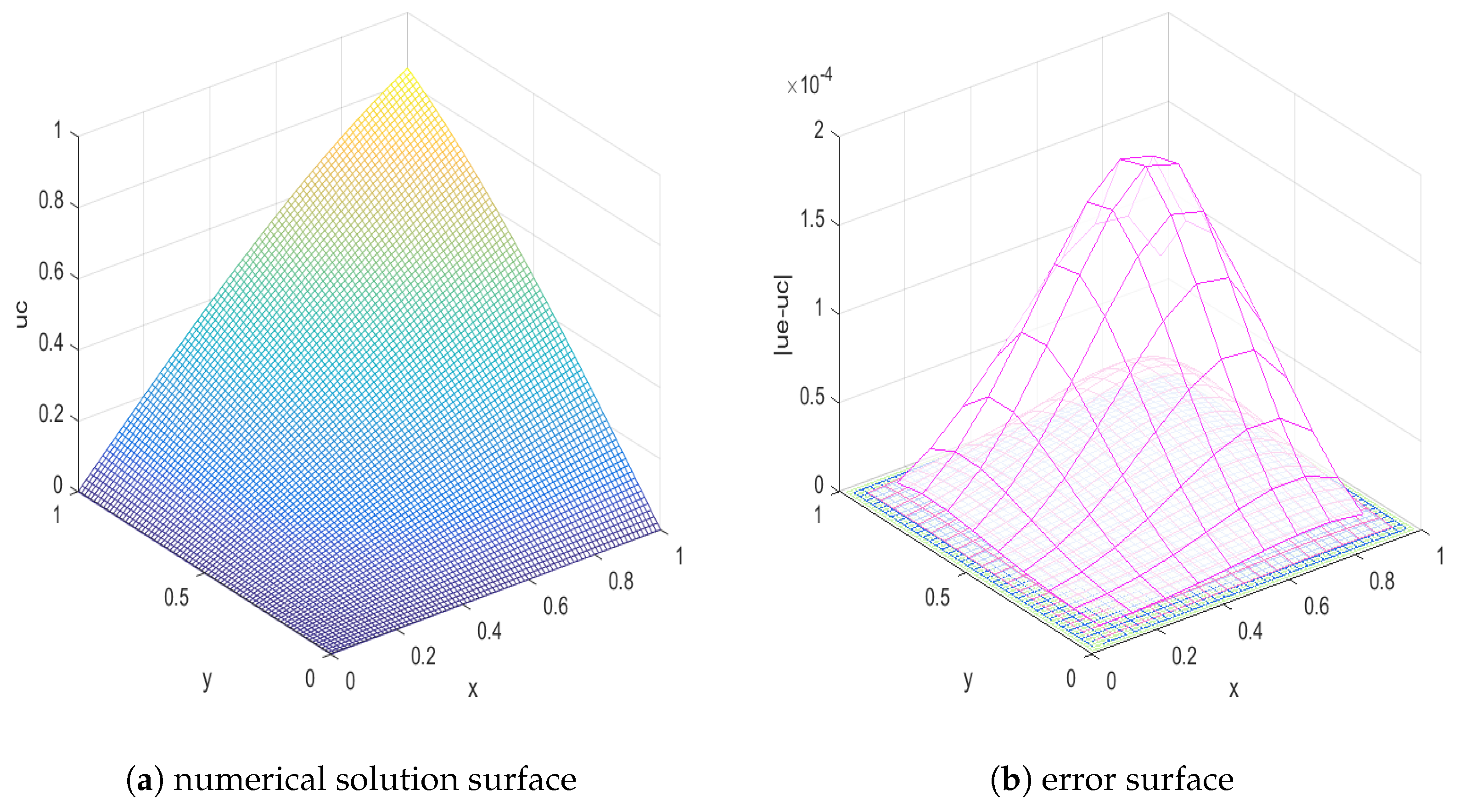
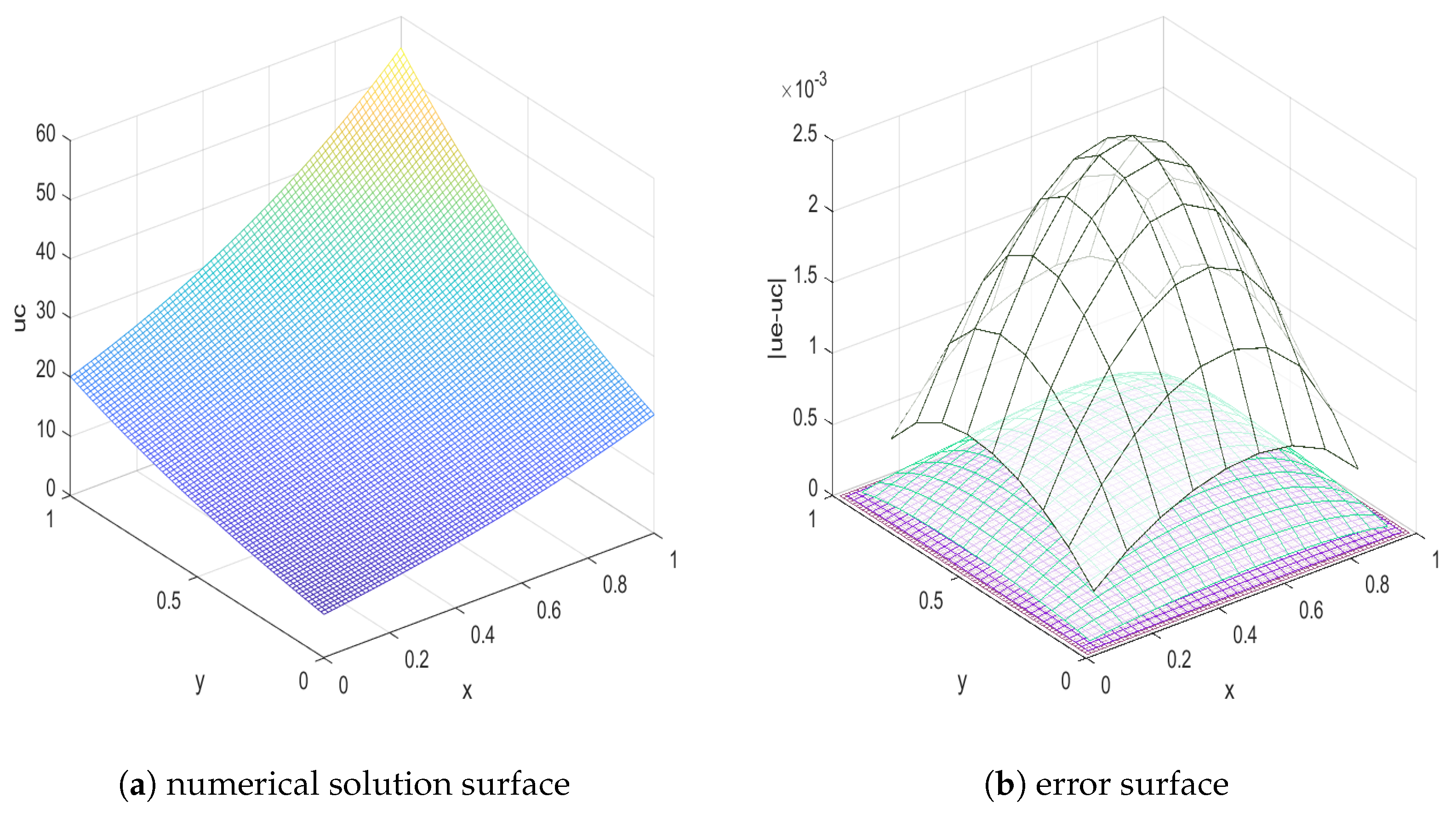
Table 1 shows the maximum error and error order of the numerical solutions for Example 1 when the difference scheme (26)–(29) is applied, and the maximum error and error order of numerical solutions when the extrapolation method is applied. Figure 1a shows the surface of the numerical solution when $t=1$; Figure 1b shows the error surface of the numerical solutions at different step sizes when $t=1$. By observing the calculation results, it can be seen that the error order of the difference scheme can be stabilized at the second order, the error order is increased to the third order after the application of the extrapolation method, and there is a tendency to increase to the fourth order with the increase in subdivision. This is slightly different from the theory, possibly due to the influence of ${(R_4)}_{ij}^k$ that is ignored in the external presumptive theory.

Table 1. Numerical results of Example 1.

Scheme	Mesh Size (h)	Mesh Size ($\mathit{\tau }$)	${\mathit{E}}_{\mathit{\infty }}\mathbf{(}\mathit{h},\mathit{\tau }\mathbf{)}$	Rate $\mathbf{(}\mathit{h},\mathit{\tau }\mathbf{)}$	Time (s)
ADI	1/10	1/100	$1.520\times {10}^{-4}$	*	0.154
	1/20	1/400	$3.950\times {10}^{-5}$	1.944	0.352
	1/40	1/1600	$9.997\times {10}^{-6}$	1.983	2.798
	1/80	1/6400	$2.505\times {10}^{-6}$	1.997	34.196
	1/10	1/100	$1.145\times {10}^{-5}$	*	*
Extrapolation	1/20	1/400	$1.097\times {10}^{-6}$	3.383	*
	1/40	1/1600	$8.762\times {10}^{-8}$	3.647	*

In the fifth column of the table, * represents none. In the sixth column of the table, * means that the time is very little and almost zero.

Figure 1. The numerical solution surface and error surface of Example 1 ($t=1$).

Example 2.

Consider the problem

$$\begin{array}{c}\hfill \left\{\begin{array}{c}{u}_t-u\Delta u=xycos(xyt)+(x^2{t}^2+y^2{t}^2){sin}^2(xyt),0<x,y<1,0<t\le 1,\hfill \\ u(x,y,0)=0,0\le x,y\le 1,\hfill \\ u(0,y,t)=0,u(1,y,t)=sin(yt),0\le y\le 1,0<t\le 1,\hfill \\ u(x,0,t)=0,u(x,1,t)=sin(xt),0\le x\le 1,0<t\le 1.\hfill \end{array}\right.\end{array}$$

(54)

exact solution $u=sin(xyt)$.

Table 2 shows the maximum error and error order of the numerical solutions for Example 2 when the difference scheme (26)–(29) is applied, and the maximum error and error order of numerical solutions when the extrapolation method is applied. Figure 2a shows the surface of the numerical solution when $t=1$, and Figure 2b shows the error surface of the numerical solutions at different step sizes when $t=1$.

Table 2. Numerical results of Example 2.

Scheme	Mesh Size (h)	Mesh Size ($\mathit{\tau }$)	${\mathit{E}}_{\mathit{\infty }}(\mathit{h},\mathit{\tau })$	Rate $(\mathit{h},\mathit{\tau })$	Time (s)
ADI	1/10	1/100	$1.617\times {10}^{-4}$	*	0.197
	1/20	1/400	$3.988\times {10}^{-5}$	2.020	0.582
	1/40	1/1600	$9.9036\times {10}^{-6}$	2.010	2.812
	1/80	1/6400	$2.477\times {10}^{-6}$	2.000	33.559
	1/10	1/100	$1.702\times {10}^{-6}$	*	*
Extrapolation	1/20	1/400	$1.118\times {10}^{-7}$	3.929	*
	1/40	1/1600	$7.064\times {10}^{-9}$	3.984	*

In the fifth column of the table, * represents none. In the sixth column of the table, * means that the time is very little and almost zero.

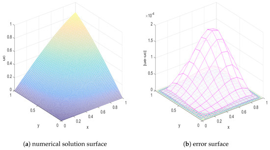
Figure 2. The numerical solution surface and error surface of Example 2 ($t=1$).

As can be seen from Table 2, when the space step size is reduced to 1/2 of the original, and the time step size is reduced to 1/4 of the original, the maximum error obtained by the ADI difference scheme is reduced to about 1/4 of the original. The maximum error obtained from the extrapolated difference scheme is reduced to about 1/16 of the original. By observing the data, it can be found that the error order of the ADI difference scheme is stable at the second order, which is consistent with the theoretical error order $O({\tau }^2+h^2)$ of Theorem 2. After applying the extrapolation method, the error order is increased to the fourth order, which is consistent with the theoretical error order $O({\tau }^4+h^4+{\tau }^2{h}^2)$ of Theorem 4.

Example 3.

Consider the problem

$$\begin{array}{c}\hfill \left\{\begin{array}{c}{u}_t=\Delta u,0<x,y<1,0<t\le 1,\hfill \\ u(x,y,0)=e^{x+y}, 0\le x,y\le 1,\hfill \\ u(0,y,t)=e^{y+2t}, u(1,y,t)=e^{1+y+2t}, 0\le y\le 1, 0<t\le 1,\hfill \\ u(x,0,t)=e^{x+2t},u(x,1,t)=e^{x+1+2t}, 0\le x\le 1, 0<t\le 1.\hfill \end{array}\right.\end{array}$$

(55)

exact solution $u=e^{x+y+2t}$.

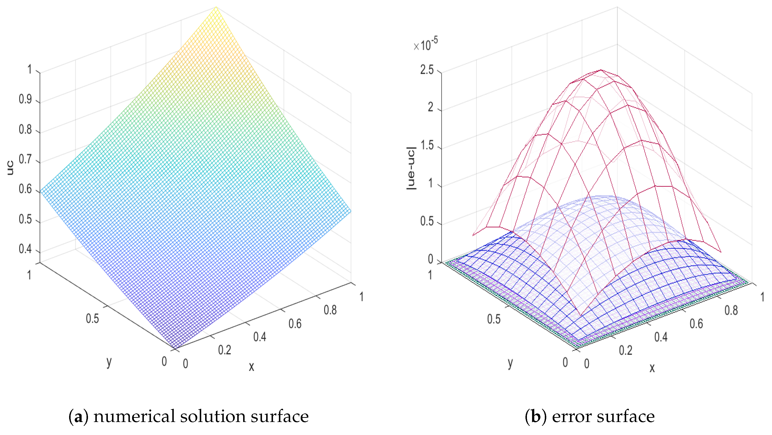
Example 3 is the example in reference [14]. We use the format proposed in this paper to solve it. Table 3 also gives the maximum error and error order of numerical solutions, as well as the calculation time for solving using the ADI scheme. Table 4 shows the maximum error of the C-N scheme proposed in reference [14] and the ADI scheme in this paper at different points when the step size $h=1/20$ and $\tau =1/800$. Figure 3a shows the surface of the numerical solution when $t=1$, Figure 3b shows the error surface of the numerical solutions at different step sizes when $t=1$. By observing the data, we can find that the convergence order obtained by applying ADI method or extrapolation method is consistent with the theory, and the calculation speed is very fast.

Table 3. Numerical results of Example 3.

Scheme	Mesh Size (h)	Mesh Size ($\mathit{tau}$)	${\mathit{E}}_{\mathit{\infty }}(\mathit{h},\mathit{\tau })$	Rate $(\mathit{h},\mathit{\tau })$	Time (s)
ADI	1/10	1/100	$2.469\times {10}^{-3}$	*	0.160
	1/20	1/400	$6.046\times {10}^{-4}$	2.030	0.493
	1/40	1/1600	$1.506\times {10}^{-4}$	2.004	2.318
	1/80	1/6400	$3.761\times {10}^{-5}$	2.002	28.769
	1/10	1/100	$1.674\times {10}^{-5}$	*	*
Extrapolation	1/20	1/400	$1.102\times {10}^{-6}$	3.925	*
	1/40	1/1600	$6.972\times {10}^{-8}$	3.983	*

In the fifth column of the table, * represents none. In the sixth column of the table, * means that the time is very little and almost zero.

Table 4. Numerical results of Example 3.

x	y	Crank–Nicolson Error	Alternating-Direction Implicit Error
0.1	0.1	$0.7\times {10}^{-4}$	$6.597\times {10}^{-5}$
0.2	0.2	$0.2\times {10}^{-3}$	$1.985\times {10}^{-4}$
0.3	0.3	$0.3\times {10}^{-3}$	$3.495\times {10}^{-4}$
0.4	0.4	$0.5\times {10}^{-3}$	$4.847\times {10}^{-4}$
0.5	0.5	$0.6\times {10}^{-3}$	$5.759\times {10}^{-4}$
0.6	0.6	$0.6\times {10}^{-3}$	$6.001\times {10}^{-4}$
0.7	0.7	$0.5\times {10}^{-3}$	$5.411\times {10}^{-4}$
0.8	0.8	$0.4\times {10}^{-3}$	$3.936\times {10}^{-4}$
0.9	0.9	$0.2\times {10}^{-3}$	$1.762\times {10}^{-4}$

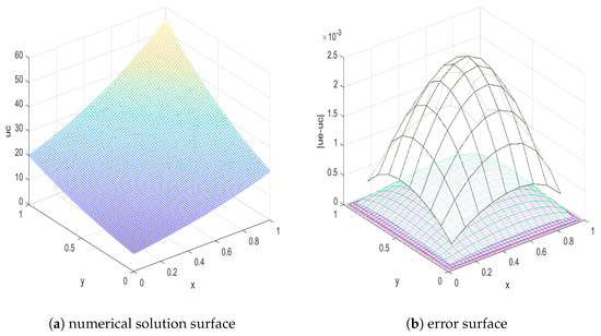
Figure 3. The numerical solution surface and error surface of Example 3 ($t=1$).

6. Conclusions

In this paper, the numerical solution for two-dimensional nonlinear parabolic equations is studied by means of an alternating-direction implicit scheme. The stability and convergence of the difference scheme are proven by using a Crank–Nicolson scheme in a time direction and energy analysis method. It is shown that the difference scheme is $L^1$ convergence, and the convergence order is $O(h_1^2+h_2^2+{\tau }^2)$. The results of the numerical examples show that the convergence order of the difference scheme is of the second order, which is consistent with the theory. After applying Richardson extrapolation, the convergence order of the difference scheme is increased to the fouth order, and the precision of the numerical solution is greatly improved. By using an ADI difference scheme for a two-dimensional problem, the CPU time is extremely small. The numerical solutions of three-dimensional nonlinear parabolic equations will be the focus of our next study.

References

- Sun, Z. Numerical Methods for Partial Differential Equations; Science Press: Beijing, China, 2005. (In Chinese) [Google Scholar]
- Khebchareon, M.; Pani, A.; Fairweather, G. Convergence analyses of crank-nicolson orthogonal spline collocation methods for linear parabolic problems in two space variables. Int. J. Numer. Anal. Model. 2016, 13, 58–72. [Google Scholar]
- Ji, C.; Du, R.; Sun, Z. Stability and convergence of difference schemes for multi-dimensional parabolic equations with variable coefficients and mixed derivatives. Int. J. Comput. Math. 2018, 95, 255–277. [Google Scholar] [CrossRef]
- Liao, H.; Sun, Z. Maximum norm error bounds of ADI and compact ADI methods for solving parabolic equations. Numer. Methods Partial. Differ. Equ. Int. J. 2010, 26, 37–60. [Google Scholar] [CrossRef]
- Liao, H.L.; Zhao, Y.; Teng, X.H. A weighted ADI scheme for subdiffusion equations. J. Sci. Comput. 2016, 69, 1144–1164. [Google Scholar] [CrossRef]
- Liao, H.L.; Sun, Z.Z.; Shi, H.S.; Wang, T.C. Convergence of compact ADI method for solving linear Schrodinger equations. Numer. Methods Partial. Differ. Equ. 2012, 28, 1598–1619. [Google Scholar] [CrossRef]
- Liao, H.L.; Li, D.; Zhang, J. Sharp error estimate of the nonuniform L1 formula for linear reaction-subdiffusion equations. Siam J. Numer. Anal. 2018, 56, 1112–1133. [Google Scholar] [CrossRef]
- Putri, E.; Shahab, M.; Iqbal, M.; Mukhlash, I. A deep-genetic algorithm (deep-GA) approach for high-dimensional nonlinear parabolic partial differential equations. Comput. Math. Appl. 2024, 154, 120–127. [Google Scholar] [CrossRef]
- Kazakov, A.; Nefedova, O.; Spevak, L. Solution to a Two-Dimensional Nonlinear Parabolic Heat Equation Subject to a Boundary Condition Specified on a Moving Manifold. Comput. Math. Math. Phys. 2024, 64, 266–284. [Google Scholar] [CrossRef]
- Sazaklioglu, A. An iterative numerical method for an inverse source problem for a multidimensional nonlinear parabolic equation. Appl. Numer. Math. 2024, 198, 428–447. [Google Scholar] [CrossRef]
- Xiao, L.; Li, M. Initial boundary value problem for a class of higher-order n-dimensional nonlinear pseudo-parabolic equations. Bound. Value Probl. 2021, 2021, 1–24. [Google Scholar] [CrossRef]
- Tan, W.; Hoang, V. High dimensional finite element method for multiscale nonlinear monotone parabolic equations. J. Comput. Appl. Math. 2019, 345, 471–500. [Google Scholar] [CrossRef]
- Eso, R.; Napirah, M.; Usman, I.; Aba, L. The Two-Dimensional Conduction Heat Transfer Equation on a Square Plate: Explicit vs. Crank-Nicolson Method in MS Excel Spreadsheet. J. Phys. Conf. Ser. 2024, 2734, 012050. [Google Scholar] [CrossRef]
- Dehghan, M. Fully implicit finite differences methods for two-dimensional diffusion with a non-local boundary condition. J. Comput. Appl. Math. 1999, 106, 255–269. [Google Scholar] [CrossRef]
- Yang, X.; Zhang, Z. On conservative, positivity preserving, nonlinear FV scheme on distorted meshes for the multi-term nonlocal Nagumo-type equations. Appl. Math. Lett. 2024, 150, 108972. [Google Scholar] [CrossRef]
- Yang, X.; Zhang, Z. Analysis of a new NFV scheme preserving DMP for two-dimensional sub-diffusion equation on distorted meshes. J. Sci. Comput. 2024, 99, 80. [Google Scholar] [CrossRef]
- Yang, X.; Zhang, H.; Zhang, Q.; Yuan, G. Simple positivity preserving nonlinear finite volume scheme for subdiffusion equations on general non-conforming distorted meshes. Nonlinear Dyn. 2022, 108, 3859–3886. [Google Scholar] [CrossRef]
- Zhang, Q.; Zhang, J.; Zhang, Z. Error estimates of invariant-preserving difference schemes for the rotation-two-component Camassa–Holm system with small energy. Calcolo 2024, 61, 9. [Google Scholar] [CrossRef]
- Zhang, Q.; Yan, T.; Xu, D.; Chen, Y. Direct/split invariant-preserving Fourier pseudo-spectral methods for the rotation-two-component Camassa–Holm system with peakon solitons. Comput. Phys. Commun. 2024, 302, 109237. [Google Scholar] [CrossRef]
- Zhang, Q. Error estimates of compact and hybrid Richardson schemes for the parabolic equation. Appl. Math. Lett. 2024, 153, 109078. [Google Scholar] [CrossRef]
- Yan, T.; Zhang, J.; Zhang, Q. Fully conservative difference schemes for the rotation-two-component Camassa–Holm system with smooth/nonsmooth initial data. Wave Motion 2024, 129, 103333. [Google Scholar] [CrossRef]
- Xue, L.; Zhang, Q. Soliton solutions of derivative nonlinear Schrodinger equations: Conservative schemes and numerical simulation. Phys. D Nonlinear Phenom. 2024, 470, 134372. [Google Scholar] [CrossRef]
- Xue, L.; Zhang, Q.; Matus, P.P. Error estimate of the conservative difference scheme for the derivative nonlinear Schrodinger equation. Appl. Math. Lett. 2025, 159, 109283. [Google Scholar] [CrossRef]
- Zhang, H.; Yang, X.; Xu, D. Unconditional convergence of linearized OSC algorithm for semilinear subdiffusion equation with non-smooth solution. Numer. Methods Partial. Differ. Equ. 2021, 37, 1361–1373. [Google Scholar] [CrossRef]
- Zhang, H.; Yang, X.; Liu, Y.; Liu, Y. An extrapolated CN-WSGD OSC method for a nonlinear time fractional reaction-diffusion equation. Appl. Numer. Math. 2020, 157, 619–633. [Google Scholar] [CrossRef]
- Yang, X.; Zhang, Z. Superconvergence analysis of a robust orthogonal Gauss collocation method for 2D fourth-order subdiffusion equations. J. Sci. Comput. 2024, 100, 62. [Google Scholar] [CrossRef]
- Wang, J.; Jiang, X.; Yang, X.; Zhang, H. A new robust compact difference scheme on graded meshes for the time-fractional nonlinear Kuramoto-Sivashinsky equation. Comput. Appl. Math. 2024, 43, 381. [Google Scholar] [CrossRef]
- Shi, Y.; Yang, X.; Zhang, Z. Construction of a new time-space two-grid method and its solution for the generalized Burgers’ equation. Appl. Math. Lett. 2024, 158, 109244. [Google Scholar] [CrossRef]
- Jiang, Y.; Chen, H. Local convergence analysis of L1-ADI scheme for two-dimensional reaction-subdiffusion equation. J. Appl. Math. Comput. 2024, 70, 1953–1964. [Google Scholar] [CrossRef]
- Jiang, Y.; Chen, H. Convergence analysis of a L1-ADI scheme for two-dimensional multiterm reaction-subdiffusion equation. Numer. Methods Partial. Differ. Equ. 2024, 40, e23115. [Google Scholar] [CrossRef]
- Jiang, Y.; Chen, H.; Sun, T.; Huang, C. Efficient L1-ADI finite difference method for the two-dimensional nonlinear time-fractional diffusion equation. Appl. Math. Comput. 2024, 471, 128609. [Google Scholar] [CrossRef]
- Wang, Z.; Cen, D.; Mo, Y. Sharp error estimate of a compact L1-ADI scheme for the two-dimensional time-fractional integro-differential equation with singular kernels. Appl. Numer. Math. 2021, 159, 190–203. [Google Scholar] [CrossRef]
- Chen, L.; Wang, Z.; Vong, S. A second-order weighted ADI scheme with nonuniform time grids for the two-dimensional time-fractional telegraph equation. J. Appl. Math. Comput. 2024, 1–18. [Google Scholar] [CrossRef]
- Qiu, W.; Xu, D.; Chen, H.; Guo, J. An alternating direction implicit Galerkin finite element method for the distributed-order time-fractional mobile–immobile equation in two dimensions. Comput. Math. Appl. 2020, 80, 3156–3172. [Google Scholar] [CrossRef]
- Guo, T.; Nikan, O.; Avazzadeh, Z.; Qiu, W. Efficient alternating direction implicit numerical approaches for multi-dimensional distributed-order fractional integro differential problems. Comput. Appl. Math. 2022, 41, 236. [Google Scholar] [CrossRef]
- Jiang, H.; Xu, D.; Qiu, W.; Zhou, J. An ADI compact difference scheme for the two-dimensional semilinear time-fractional mobile–immobile equation. Comput. Appl. Math. 2020, 39, 1–17. [Google Scholar] [CrossRef]
- Luo, M.; Qiu, W.; Nikan, O.; Avazzadeh, Z. Second-order accurate, robust and efficient ADI Galerkin technique for the three-dimensional nonlocal heat model arising in viscoelasticity. Appl. Math. Comput. 2023, 440, 127655. [Google Scholar] [CrossRef]
- Qiu, W.; Nikan, O.; Avazzadeh, Z. Numerical investigation of generalized tempered-type integrodifferential equations with respect to another function. Fract. Calc. Appl. Anal. 2023, 26, 2580–2601. [Google Scholar] [CrossRef]
- Qiu, W.; Li, Y.; Zheng, X. Numerical analysis of nonlinear Volterra integrodifferential equations for viscoelastic rods and plates. Calcolo 2024, 61, 50. [Google Scholar] [CrossRef]
- Qiao, L.; Qiu, W.; Xu, D. Error analysis of fast L1 ADI finite difference/compact difference schemes for the fractional telegraph equation in three dimensions. Math. Comput. Simul. 2023, 205, 205–231. [Google Scholar] [CrossRef]
- Qiao, L.; Guo, J.; Qiu, W. Fast BDF2 ADI methods for the multi-dimensional tempered fractional integrodifferential equation of parabolic type. Comput. Math. Appl. 2022, 123, 89–104. [Google Scholar] [CrossRef]
- Qiao, L.; Qiu, W.; Xu, D. Crank-Nicolson ADI finite difference/compact difference schemes for the 3D tempered integrodifferential equation associated with Brownian motion. Numer. Algorithms 2023, 93, 1083–1104. [Google Scholar] [CrossRef]
- Qiao, L.; Qiu, W.; Tang, B. A fast numerical solution of the 3D nonlinear tempered fractional integrodifferential equation. Numer. Methods Partial. Differ. Equ. 2023, 39, 1333–1354. [Google Scholar] [CrossRef]
- Li, C.; Zhang, H.; Yang, X. A fourth-order accurate extrapolation nonlinear difference method for fourth-order nonlinear PIDEs with a weakly singular kernel. Comput. Appl. Math. 2024, 43, 288. [Google Scholar] [CrossRef]
- Yang, X.; Qiu, W.; Chen, H.; Zhang, H. Second-order BDF ADI Galerkin finite element method for the evolutionary equation with a nonlocal term in three-dimensional space. Appl. Numer. Math. 2022, 22, 497–513. [Google Scholar] [CrossRef]
- Yang, X.; Qiu, W.; Zhang, H.; Tang, L. An efficient alternating direction implicit finite difference scheme for the three-dimensional time-fractional telegraph equation. Comput. Math. Appl. 2021, 102, 233–247. [Google Scholar] [CrossRef]
- Cao, D.; Chen, H. Pointwise-in-time error estimate of an ADI scheme for two-dimensional multi-term subdiffusion equation. J. Appl. Math. Comput. 2023, 69, 707–729. [Google Scholar] [CrossRef]
- Li, K.; Chen, H.; Xie, S. Error estimate of L1-ADI scheme for two-dimensional multi-term time fractional diffusion equation. Netw. Heterog. Media 2023, 18, 1454–1470. [Google Scholar] [CrossRef]
- Wang, Y.; Chen, H. Pointwise error estimate of an alternating direction implicit difference scheme for two-dimensional time-fractional diffusion equation. Comput. Math. Appl. 2021, 99, 155–161. [Google Scholar] [CrossRef]
- Wang, Y.; Chen, H.; Sun, T. α-robust H1-norm convergence analysis of ADI scheme for two-dimensional time-fractional diffusion equation. Appl. Numer. Math. 2021, 168, 75–83. [Google Scholar] [CrossRef]
- Burg, C.; Erwin, T. Application of Richardson extrapolation to the numerical solution of partial differential equations. Numer. Methods Partial. Differ. Equ. 2009, 25, 810–832. [Google Scholar] [CrossRef]
Disclaimer/Publisher’s Note: The statements, opinions and data contained in all publications are solely those of the individual author(s) and contributor(s) and not of MDPI and/or the editor(s). MDPI and/or the editor(s) disclaim responsibility for any injury to people or property resulting from any ideas, methods, instructions or products referred to in the content. |
© 2024 by the authors. Licensee MDPI, Basel, Switzerland. This article is an open access article distributed under the terms and conditions of the Creative Commons Attribution (CC BY) license (https://creativecommons.org/licenses/by/4.0/).