Enhanced Subspace Iteration Technique for Probabilistic Modal Analysis of Statically Indeterminate Structures

Abstract

In structural stochastic dynamic analysis, the consideration of the randomness in the physical parameters of the structure necessitates the establishment of numerous stochastic finite element models and the subsequent computation of their corresponding vibration modes. When the complete analysis is applied to calculate the vibration modes for each sample of the stochastic finite element model, a substantial computational expense is incurred. To enhance computational efficiency, this work presents an extended subspace iteration method aimed at rapidly determining the vibration modal parameters of statically indeterminate structures. The essence of this proposed method revolves around efficiently constructing reduced basis vectors during the subspace iteration process, utilizing flexibility disassembly perturbation and the Krylov subspace. This extended subspace iteration method proves particularly advantageous for the modal analysis of finite element models that incorporate a multitude of random variables. The proposed modal random analysis method has been validated using both a truss structure and a beam structure. The results demonstrate that the proposed method achieves substantial savings in computational time. Specifically, for the truss structure, the calculation time of the proposed method is approximately 1.2% and 65% of that required by the comprehensive analysis method and the combined approximation method, respectively. For the beam structure, on average, the computational time of the proposed method is roughly 2.1% of a full analysis and approximately 48.2% of the Ritz vector method’s time requirement. Compared to existing stochastic modal analysis algorithms, the proposed method offers improved computational accuracy and efficiency, particularly in scenarios involving high-discreteness random analyses.

1. Introduction

The material properties and geometric dimensions of a real engineering structure are random [1,2,3]. Therefore, the finite element model (FEM) containing many random variables is more in line with the real situation of a structure. When considering the randomness of the structure, it is usually necessary to take thousands of FEM samples and calculate the corresponding static or dynamic response to analyze the reliability of the structure. Taking dynamic modal analysis as an example, the common methods for solving dynamic eigenvalue problems include the inverse iteration (II) method [4,5], the subspace iteration (SI) method [6,7], model reduction [8], and so on. Among them, the subspace iteration method is the most widely used due to its computational efficiency and ease of programming. Lin and Simoncini [9] applied the subspace iteration method to solve the continuous algebraic Riccati equation. Gu [10] considered randomness within the framework of the subspace iteration method and proposed a new error analysis method. Lasecka and Lewandowski [11] extended the subspace iteration method and applied it to systems of viscoelastic damping elements described by both classical and fractional models. However, for a structure with over ten thousand degrees of freedom (DOFs), conducting a complete dynamic modal analysis generally requires a significant computational cost based on the above methods. If thousands of samples are taken, using the above methods to calculate the modal parameters of each FEM sample will require a huge amount of computation, which may make the stochastic dynamic analysis difficult to carry out. Thus, many dynamic modal reanalysis methods have been proposed in recent years to fast calculate the modal parameters of a random structure based on the modal data of the original structure. Chen et al. [12,13] performed a comparative analysis evaluating the computational efficiency of the matrix perturbation, combined approximation (CA), and extended CA algorithms. Following this, Kirsch et al. [14,15] integrated CA with II and SI techniques for the reanalysis of structural vibrations. Yang et al. [16] applied the CA algorithm in dynamic reanalysis, focusing on various topology revision scenarios. Hong et al. [17] introduced a condensation model that expedited the recalculation of modified modal data through substructure combination. Xu et al. [18] enhanced the CA algorithm for dynamic reanalysis by incorporating the frequency-shift process. Norouzi et al. [19] utilized reanalysis algorithms to assess the fatigue life of structures. Mourelatos et al. [20] conducted dynamic reanalysis of large-scale structures, leveraging model reduction and the CA algorithm. Zheng et al. [21] combined CA with frequency-shift to rapidly compute the modal data of revised structures. Liu et al. [22] solved the modal reanalysis problem post-structural revision using the modal synthesis algorithm. Li et al. [23] facilitated aircraft design through the application of the modal reanalysis algorithm. Zheng et al. [24] explored the modal reanalysis method in response to an increase in structural degrees of freedom. Huang et al. [25] performed displacement and modal reanalysis of structures with nonlinear boundary conditions. He et al. [26,27] devised a dynamic reanalysis method that fused pseudo-random number initialization, independent and coupled II, and Rayleigh–Ritz analysis. Chang et al. [28] developed an SMW formula-based model reduction algorithm for structural modal reanalysis. Recently, Li et al. [29] investigated the modal reanalysis of large structural modifications incorporating local nonlinearity.

Despite notable strides in dynamic reanalysis, the prevailing methodologies continue to grapple with limitations, notably low computational precision and instability in complex stochastic dynamic assessments involving myriad random parameters. In this context, the emergence of flexibility disassembly perturbation (FDP) [30,31] as a game-changer for static structural analyses is significant. FDP has demonstrated remarkable effectiveness in static reanalysis [30] and static sensitivity reanalysis [31] of large-scale, high-complexity scenarios. Driven by the achievements, FDP is employed in this work to strengthen the subspace iteration algorithm, making it capable of performing dynamic random analysis on large-scale, statically indeterminate structures. The essence of this method lies in swiftly generating reduced basis vectors during subspace iteration, leveraging flexibility disassembly perturbation and Krylov subspace techniques for enhanced efficiency. This innovative modal stochastic analysis approach, validated through a truss structure, outperforms conventional methods in terms of computational efficiency and stability. The article is structured as follows: Section 2 initially offers a concise review of the subspace iteration algorithm’s calculation steps and key formulas utilized in modal computation. Subsequently, FDP is implemented to enhance the subspace iteration method, specifically tailored for conducting modal random analysis on individual FEM samples of the structure. Section 3 showcases a numerical illustration to validate the proposed method and benchmark it against existing approaches. Lastly, Section 4 summarizes the key takeaways and contributions of this research endeavor.

2. Theoretical Development

2.1. Subspace Iteration Method for Vibration Modal Computation

For a $n$-DOF structure, the modal parameters of free vibration can be obtained by the eigen-pair equation as:

$$K\mathsf{\Psi }=M\mathsf{\Psi }\mathsf{\Lambda }$$

(1)

$${\mathsf{\Psi }}^{T}M\mathsf{\Psi }=I$$

(2)

$$\mathsf{\Psi }=[{\varphi }_1,\cdots ,{\varphi }_q]$$

(3)

$$\mathsf{\Lambda }=\left[\begin{array}{ccc}{\lambda }_1& & \\ & \ddots & \\ & & {\lambda }_q\end{array}\right]$$

(4)

where $K$ and $M$ denote the $n\times n$ dimensional stiffness and mass matrices of the initial FEM; $\mathsf{\Psi }$ is the eigenvector matrix; $\mathsf{\Lambda }$ is a diagonal matrix of eigenvalues; ${\lambda }_1,\cdots ,{\lambda }_q$ and ${\varphi }_1,\cdots ,{\varphi }_q$ denote the first $q$ eigenvalues and eigenvectors; and $I$ denotes an identity matrix. The subspace iteration method is the most commonly used algorithm for solving the above dynamic eigen-pair problem, which can compute $q$ low-order eigen-pairs at once. The main steps of the subspace iteration method are as follows:

Step 1. Construct an initial eigenvector matrix ${\mathsf{\Psi }}^{(0)}$ using $s$ linearly independent vectors. The parameter $s$ should be greater than the number of desired eigenvalue pairs $q$. Based on existing research [6,7], $s$ can be taken as the smaller value between $2q$ and $q+8$, i.e., $s=\min (2q, q+8)$.

Step 2. For the $i$-th iteration, calculate the new eigenvector matrix ${\overline{\mathsf{\Psi }}}^{(i)}$ through:

$${\overline{\mathsf{\Psi }}}^{(i)}=K^{-1}M{\mathsf{\Psi }}^{(i-1)}$$

(5)

In Equation (5), $K^{-1}$ represents the inverse matrix of $K$.

Step 3. Calculate the condensed stiffness matrix $K_R$ and mass matrix $M_R$ through:

$$K_R={({\overline{\mathsf{\Psi }}}^{(i)})}^{T}K{\overline{\mathsf{\Psi }}}^{(i)}$$

(6)

$$M_R={({\overline{\mathsf{\Psi }}}^{(i)})}^{T}M{\overline{\mathsf{\Psi }}}^{(i)}$$

(7)

Step 4. Solve the simplified eigen-pair problem of the $s\times s$ reduced system to achieve the corresponding eigenvalues ${\mathsf{\Lambda }}^{(i)}$ and eigenvectors $Y^{(i)}$ as follows:

$$K_R{Y}^{(i)}=M_R{Y}^{(i)}{\mathsf{\Lambda }}^{(i)}$$

(8)

Step 5. For the $i$-th iteration, the solution of the eigenvalues of the original system is ${\mathsf{\Lambda }}^{(i)}$. The solution of the eigenvectors of the original system is calculated through:

$${\mathsf{\Psi }}^{(i)}={\overline{\mathsf{\Psi }}}^{(i)}{Y}^{(i)}$$

(9)

Step 6. The iteration can be terminated when the results of two adjacent iterations are very close.

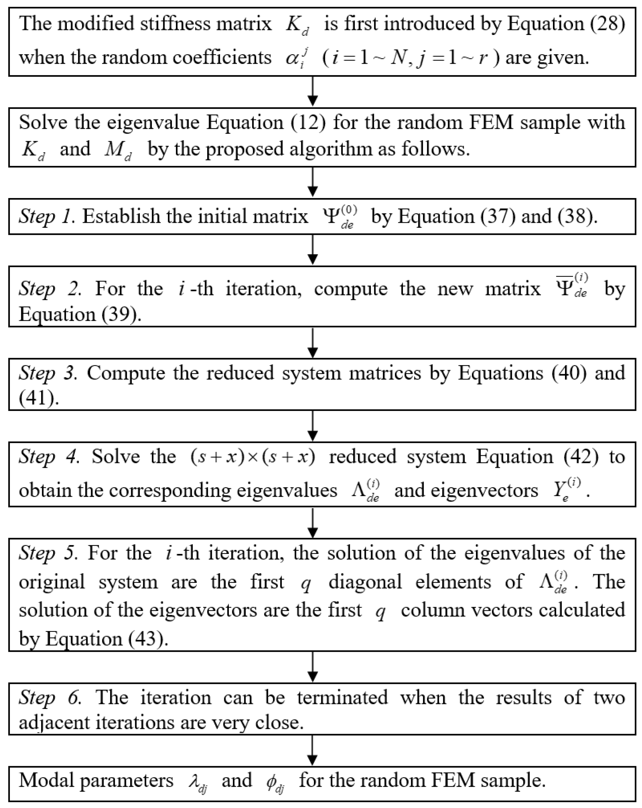
2.2. Extended Subspace Iteration Method Using FDP

For stochastic modal analysis, the stiffness and mass matrices of the structure are both random matrices due to the randomness of physical parameters such as elastic modulus and density of the material. For each random sampling, the modified stiffness matrix $K_d$ and mass matrix $M_d$ can be expressed as follows:

$$K_d=K+\mathsf{\Delta }K$$

(10)

$$M_d=M+\mathsf{\Delta }M$$

(11)

where $\mathsf{\Delta }K$ and $\mathsf{\Delta }M$ are variations caused by structural randomness. The modal eigen-pairs of this sample can also be obtained by solving the following generalized eigenvalue problem:

$$K_d{\mathsf{\Psi }}_d=M_d{\mathsf{\Psi }}_d{\mathsf{\Lambda }}_d$$

(12)

$${\mathsf{\Psi }}_d^T{M}_d{\mathsf{\Psi }}_d=I$$

(13)

$${\mathsf{\Psi }}_d=[{\varphi }_{d1},\cdots ,{\varphi }_{dq}]$$

(14)

$${\mathsf{\Lambda }}_d=\left[\begin{array}{c}{\lambda }_{d1}\\ & \ddots \\ & & {\lambda }_{dq}\end{array}\right]$$

(15)

Similarly, the complete analysis by the subspace iteration method for this FEM sample is as follows:

Step 1. Construct an initial eigenvector matrix ${\mathsf{\Psi }}_d^{(0)}$ using $s$ linearly independent vectors ($s=\min (2q, q+8)$).

Step 2. For the $i$-th iteration, calculate the new eigenvector matrix ${\overline{\mathsf{\Psi }}}_d^{(i)}$ through:

$${\overline{\mathsf{\Psi }}}_d^{\left(i\right)}=K_d^{-1}{M}_d{\mathsf{\Psi }}_d^{(i-1)}$$

(16)

Step 3. Calculate the condensed stiffness matrix $K_R$ and mass matrix $M_R$ through:

$$K_{\mathit{R}}={\left({\overline{\mathsf{\Psi }}}_d^{\left(i\right)}\right)}^T{K}_d{\overline{\mathsf{\Psi }}}_d^{\left(i\right)}$$

(17)

$$M_{\mathit{R}}={\left({\overline{\mathsf{\Psi }}}_d^{\left(i\right)}\right)}^T{M}_d{\overline{\mathsf{\Psi }}}_d^{\left(i\right)}$$

(18)

Step 4. Solve the simplified eigen-pair problem of the $s\times s$ reduced system to obtain the corresponding eigenvalues ${\mathsf{\Lambda }}^{(i)}$ and eigenvectors $Y^{(i)}$ as follows:

$$K_R{Y}^{\left(i\right)}=M_R{Y}^{\left(i\right)}{\mathsf{\Lambda }}_d^{\left(i\right)}$$

(19)

Step 5. For the $i$-th iteration, the solution of the eigenvalues of the random system is ${\mathsf{\Lambda }}_d^{\left(i\right)}$. The solution of the eigenvectors of the random system is calculated through:

$${\mathsf{\Psi }}_d^{(i)}={\overline{\mathsf{\Psi }}}_d^{(i)}{Y}^{(i)}$$

(20)

Step 6. The iteration can be terminated when the results of two adjacent iterations are very close.

Analyzing the outlined steps, it becomes evident that the primary computational bottleneck stems from the inverting matrix $K_d$ in Equation (16). When dealing with thousands of samples, this task becomes overwhelmingly intensive, potentially rendering random modal analysis unfeasible. To address this, we employ the Flexibility Disassembly Perturbation (FDP) formula, which swiftly approximates $K_d^{-1}$, significantly boosting the computational speed of the subspace iteration method. FDP’s cornerstone lies in transforming random physical parameters into a diagonal matrix by cleverly decomposing and combining elementary stiffness matrices. For this purpose, the overall stiffness matrix of the structure is elegantly represented by the cumulative sum of the elementary stiffness matrices as follows:

$$K={\displaystyle \sum _{i=1}^N{K}_i}$$

(21)

where $K_i$ denotes the $i$-th elementary stiffness matrix, $i=1~N$. The spectral decomposition of $K_i$ can be expressed as follows:

$$K_i=C_i{P}_i{C}_i^T=[c_i^1,\cdots ,c_i^r]\left[\begin{array}{ccc}{p}_i^1& & \\ & \ddots & \\ & & p_i^r\end{array}\right]{[c_i^1,\cdots ,c_i^r]}^T$$

(22)

where $p_i^1,\cdots ,p_i^r$ are the $r$ non-zero eigenvalues of $K_i$, and $c_i^1,\cdots ,c_i^r$ are the corresponding eigenvectors. For instance, performing the spectral decomposition on a plane beam–element stiffness matrix in a local coordinate system is performed as follows [28]:

$$P_i=\left[\begin{array}{ccc}{\displaystyle \frac{2EA}{L}}& 0& 0\\ 0& {\displaystyle \frac{2E{I}_m}{L}}& 0\\ 0& 0& {\displaystyle \frac{6E{I}_m(L^2+4)}{L^3}}\end{array}\right]$$

(23)

$$C_i=\left[\begin{array}{ccc}{\displaystyle \frac{1}{\sqrt{2}}}& 0& 0\\ 0& 0& {\displaystyle \frac{\sqrt{2}}{\sqrt{L^2+4}}}\\ 0& {\displaystyle \frac{-1}{\sqrt{2}}}& {\displaystyle \frac{L}{\sqrt{2}\sqrt{L^2+4}}}\\ {\displaystyle \frac{-1}{\sqrt{2}}}& 0& 0\\ 0& 0& {\displaystyle \frac{-\sqrt{2}}{\sqrt{L^2+4}}}\\ 0& {\displaystyle \frac{1}{\sqrt{2}}}& {\displaystyle \frac{L}{\sqrt{2}\sqrt{L^2+4}}}\end{array}\right]$$

(24)

In Equation (23), $E$ represents the modulus of elasticity; $A$ signifies the cross-sectional area; $I_m$ denotes the moment of inertia; and $L$ stands for the length of the beam element. Notably, the random parameters are consolidated within the diagonal elements of the matrix $P_i$. Substituting Equation (22) into (21) yields the following:

$$K=CP{C}^T$$

(25)

$$C=[c_1^1,\cdots ,c_1^r,c_2^1,\cdots ,c_2^r,\cdots ,c_N^r]$$

(26)

$$P=\left[\begin{array}{ccccc}{p}_1^1& & & & \\ & \ddots & & & \\ & & p_1^r& & \\ & & & \ddots & \\ & & & & p_N^r\end{array}\right]$$

(27)

In Equation (25), $C$ and $P$ are $n\times rN$ and $rN\times rN$ dimensional matrices, respectively. Notably, $C$ assumes a square form with dimensionality $n=rN$ for statically determinate structures, while it adopts a rectangular shape with $n<rN$ dimensions for statically indeterminate structures. Typically, stochastic variables such as the elastic modulus and cross-sectional size solely impact the diagonal matrix $P$, leading to its variation. Consequently, the revised stiffness matrix $K_d$ can be formulated as a function of these altered diagonal elements:

$$K_d=C{P}_d{C}^T$$

(28)

$$P_d=\left[\begin{array}{ccccc}{p}_1^1(1+{\alpha }_1^1)& & & & \\ & \ddots & & & \\ & & p_1^r(1+{\alpha }_1^r)& & \\ & & & \ddots & \\ & & & & p_N^r(1+{\alpha }_N^r)\end{array}\right]$$

(29)

where ${\alpha }_i^j$ ($i=1~N,j=1~r$) are the random coefficients. It is a well-established fact that the structural flexibility matrix serves as the inverse of the stiffness matrix, i.e.,

$$F\cdot K=I$$

(30)

$$F_d\cdot K_d=I$$

(31)

It is noted that the matrix $P_d$ in Equation (29) is a diagonal square matrix of dimension $rN\times rN$, and each diagonal element in $P_d$ is not equal to zero because the probability that the random coefficient ${\alpha }_i^j$ exactly equals −1 in random sampling is almost zero. Therefore, the matrix $P_d$ is invertible. For a statically determinate structure, the FDP formula can be straightforwardly derived from Equation (28), offering a simplified and direct path to its computation as follows:

$$F_d=K_d^{-1}=D{Q}_d{D}^T$$

(32)

$$D={(C^{-1})}^T$$

(33)

$$Q_d=P_d^{-1}=\left[\begin{array}{ccccc}{\displaystyle \frac{1}{p_1^1(1+{\alpha }_1^1)}}& & & & \\ & \ddots & & & \\ & & {\displaystyle \frac{1}{p_1^r(1+{\alpha }_1^r)}}& & \\ & & & \ddots & \\ & & & & {\displaystyle \frac{1}{p_N^r(1+{\alpha }_N^r)}}\end{array}\right]$$

(34)

For a statically indeterminate structure, a generalized FDP formula is developed from Equation (28) with the help of the matrix generalized inverse:

$$\overline{F_d}=K_d^{+}=\overline{D}{Q}_d{\overline{D}}^T$$

(35)

$$\overline{D}={(C^T)}^{+}={(C{C}^T)}^{-1}C$$

(36)

The superscript “+” represents the matrix generalized inverse, and it is evident that for a statically determinate structure, Equation (35) reduces to Equation (32). The FDP formulas, as shown in Equation (35), are used for fast estimating $K_d^{-1}$ in the subspace iteration method to improve the computational efficiency of random modal reanalysis. For statically indeterminate structures, since Equation (35) is an approximate estimate of $K_d^{-1}$, it is usually necessary to add extra basis vectors to the initial subspace ${\mathsf{\Psi }}_d^{(0)}$ to construct a new subspace to further improve the calculation accuracy. The extended subspace is designed as follows:

$${\mathsf{\Psi }}_{de}^{(0)}=[{\varphi }_1,{\varphi }_2,\cdots ,{\varphi }_s,{\eta }_{s+1},\cdots ,{\eta }_{s+x}], 1\le x\le s$$

(37)

where ${\varphi }_1,{\varphi }_2,\cdots ,{\varphi }_s$ are the eigenvectors of the original system without considering randomness; ${\eta }_{s+1},\cdots ,{\eta }_{s+x}$ are the added basis vectors; and $x$ is a positive integer less than $s$. These added basis vectors are calculated based on FDP and Krylov’s subspace as follows:

$${\eta }_{s+x}=\overline{F_d}{K}_d{\varphi }_x$$

(38)

Using FDP and the extended subspace, the operational process of the extended subspace iteration algorithm for random modal analysis of a statically indeterminate structure is as follows:

(1)

Construct an initial subspace matrix ${\mathsf{\Psi }}_{de}^{(0)}$ using Equations (37) and (38).

(2)

For the $i$-th iteration, calculate the new eigenvector matrix ${\overline{\mathsf{\Psi }}}_{de}^{(i)}$ using Equation (35) as follows:

$${\overline{\mathsf{\Psi }}}_{de}^{(i)}=\overline{F_d}{M}_d{\mathsf{\Psi }}_{de}^{(i-1)}$$

(39)

(3)

Calculate the condensed stiffness matrix $K_R$ and mass matrix $M_R$ through:

$$K_R={({\overline{\mathsf{\Psi }}}_{de}^{(i)})}^T{K}_d{\overline{\mathsf{\Psi }}}_{de}^{(i)}$$

(40)

$$M_R={({\overline{\mathsf{\Psi }}}_{de}^{(i)})}^T{M}_d{\overline{\mathsf{\Psi }}}_{de}^{(i)}$$

(41)

(4)

Solve the simplified eigen-pair problem of the $(s+x)\times (s+x)$ reduced system to obtain the corresponding eigenvalues ${\mathsf{\Lambda }}_{de}^{(i)}$ and eigenvectors $Y_e^{(i)}$ as follows:

$$K_R{Y}_e^{(i)}=M_R{Y}_e^{(i)}{\mathsf{\Lambda }}_{de}^{(i)}$$

(42)

(5)

For the $i$-th iteration, the solution of the eigenvalues of the random system are the first $q$ diagonal elements of ${\mathsf{\Lambda }}_{de}^{(i)}$. The solution of the eigenvectors is the first $q$ column vector obtained through:

$${\mathsf{\Psi }}_{de}^{(i)}={\overline{\mathsf{\Psi }}}_{de}^{(i)}{Y}_e^{(i)}$$

(43)

(6)

The iteration can be terminated when the results of two adjacent iterations are very close.

Figure 1 shows the operation flow of the proposed random modal analysis method for statically indeterminate structures more intuitively.

3. Numerical Examples

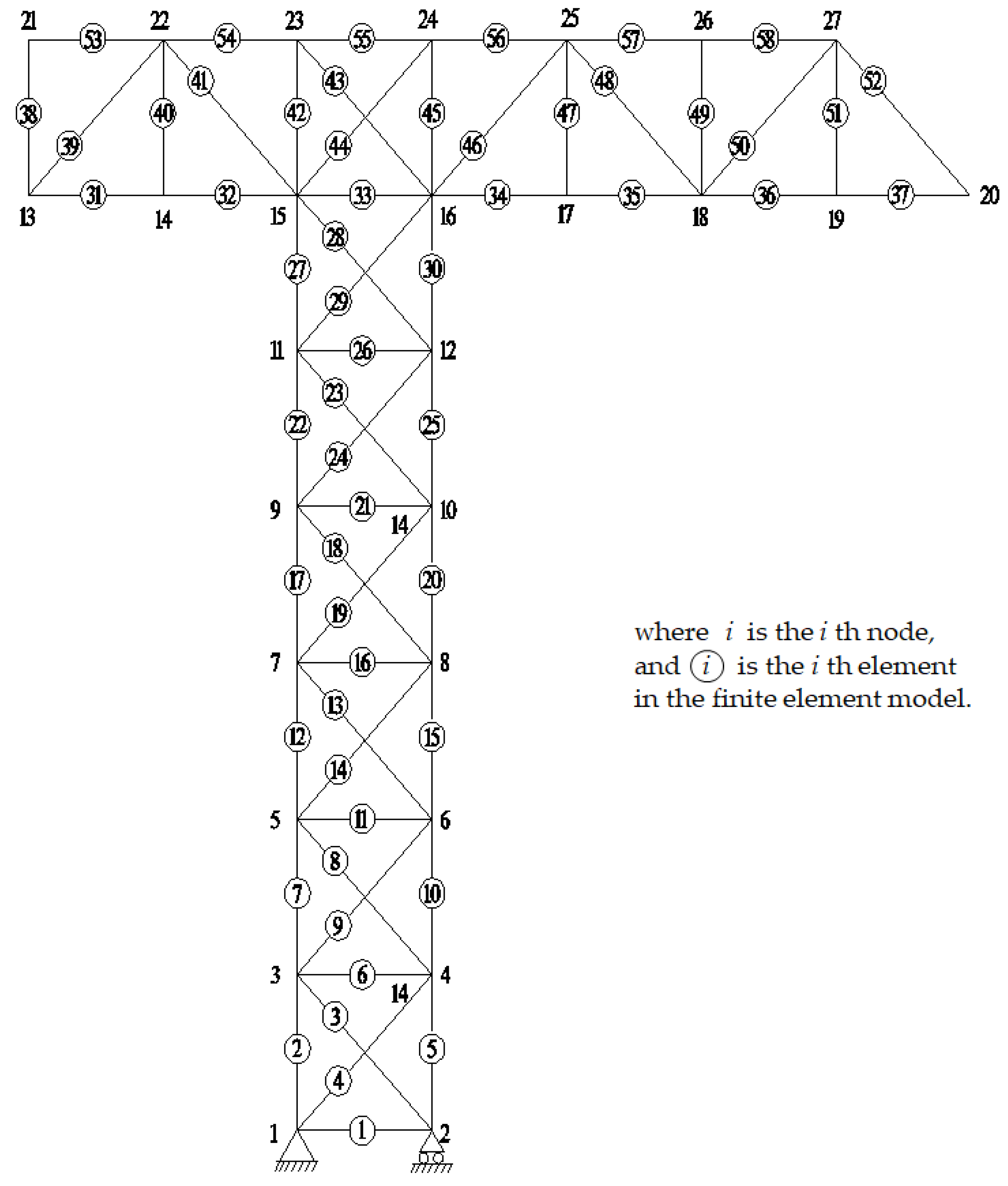
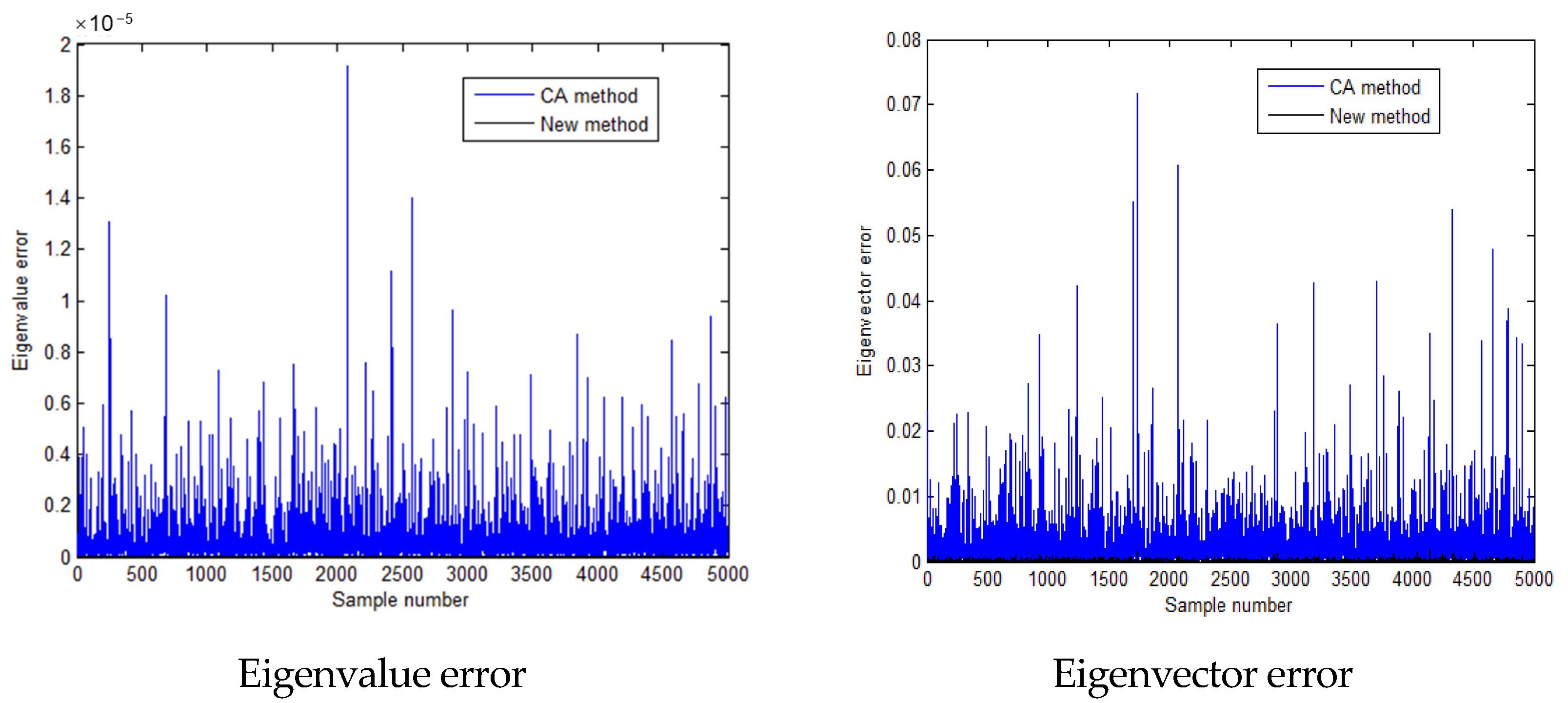
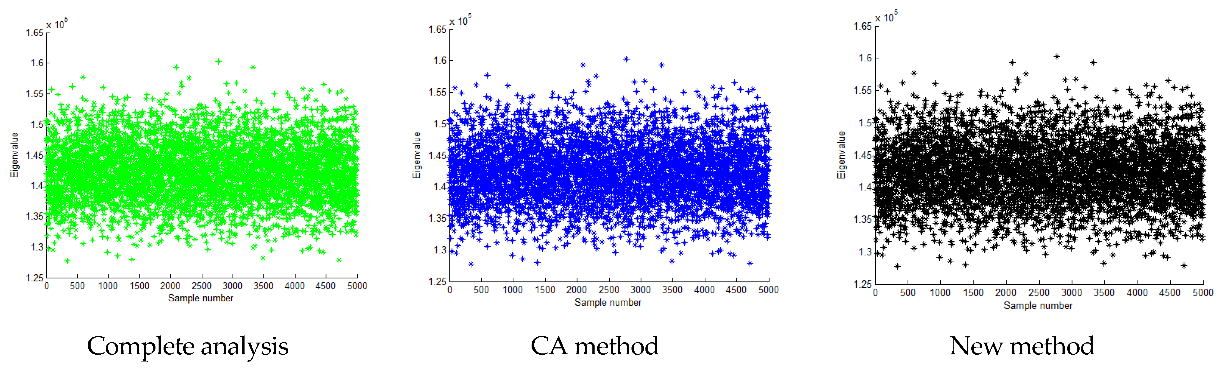
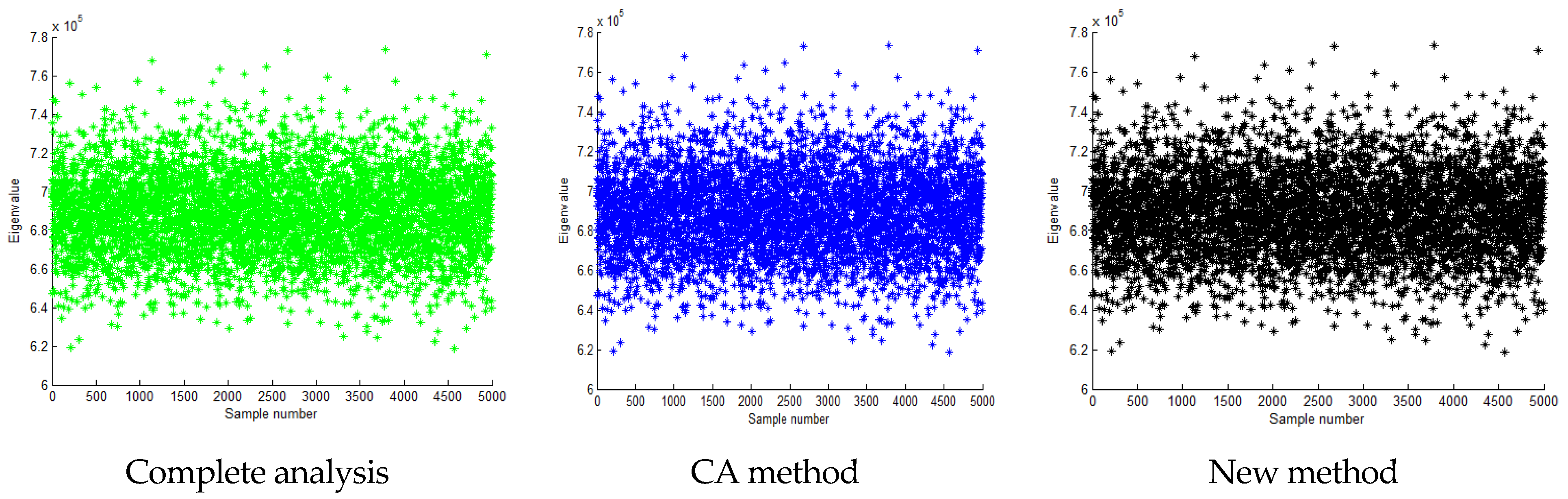
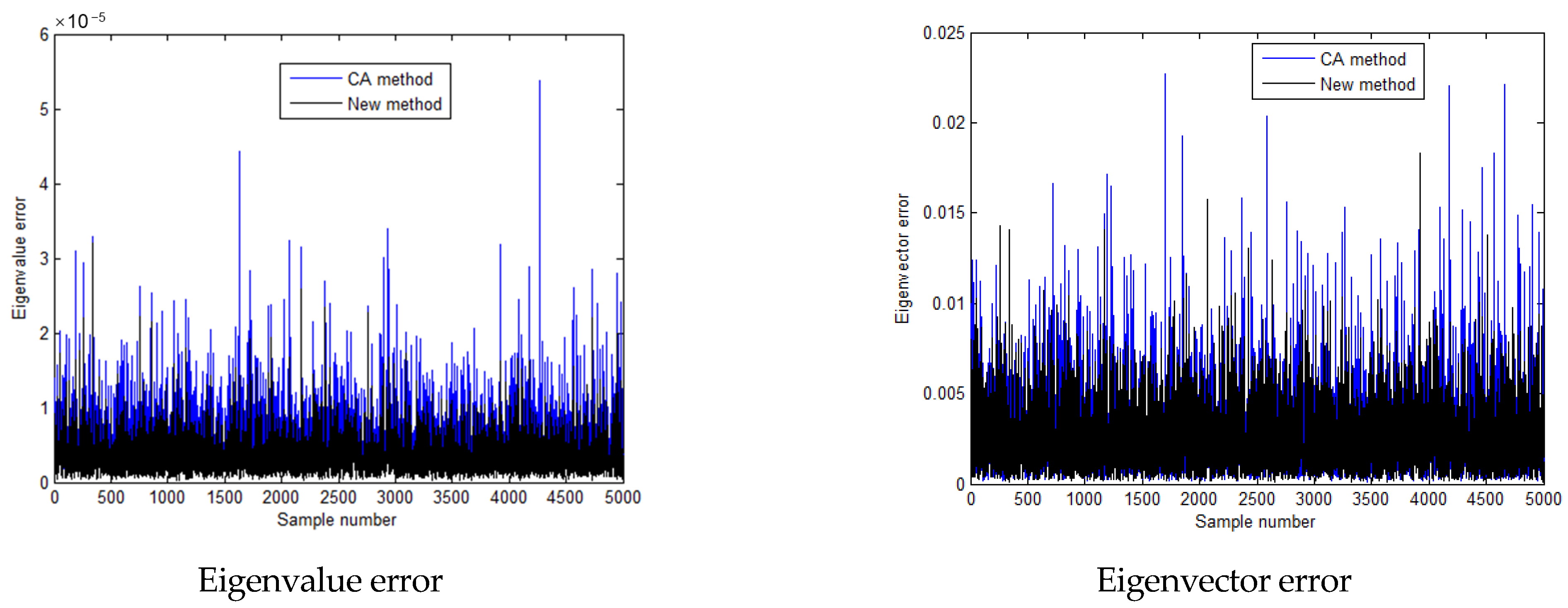
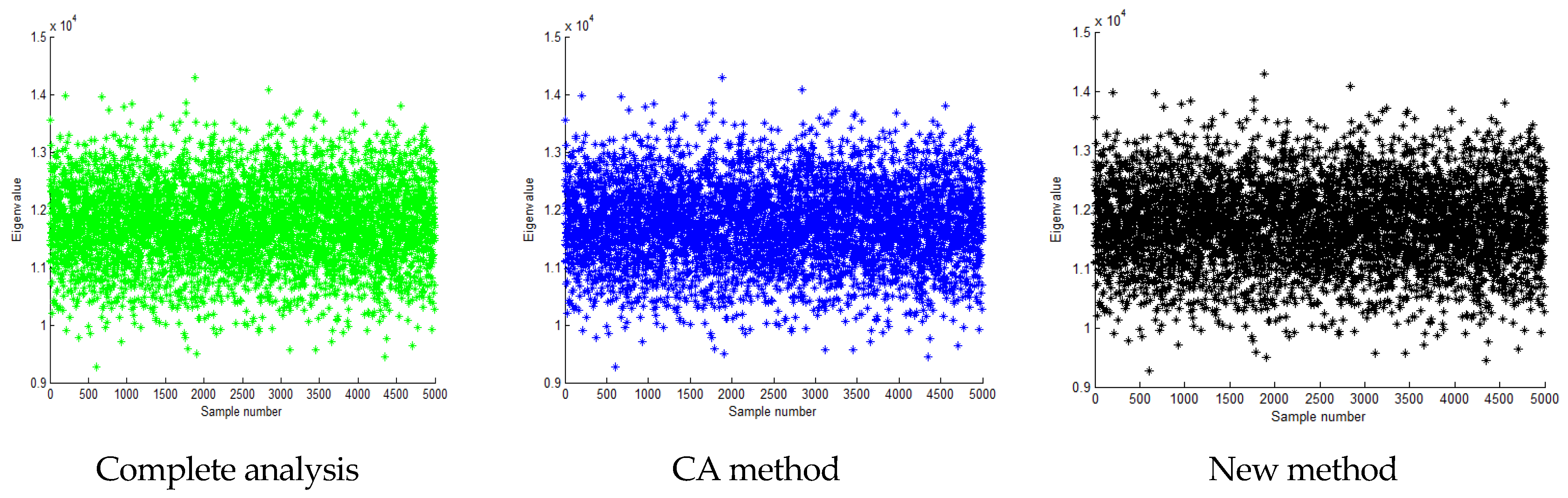
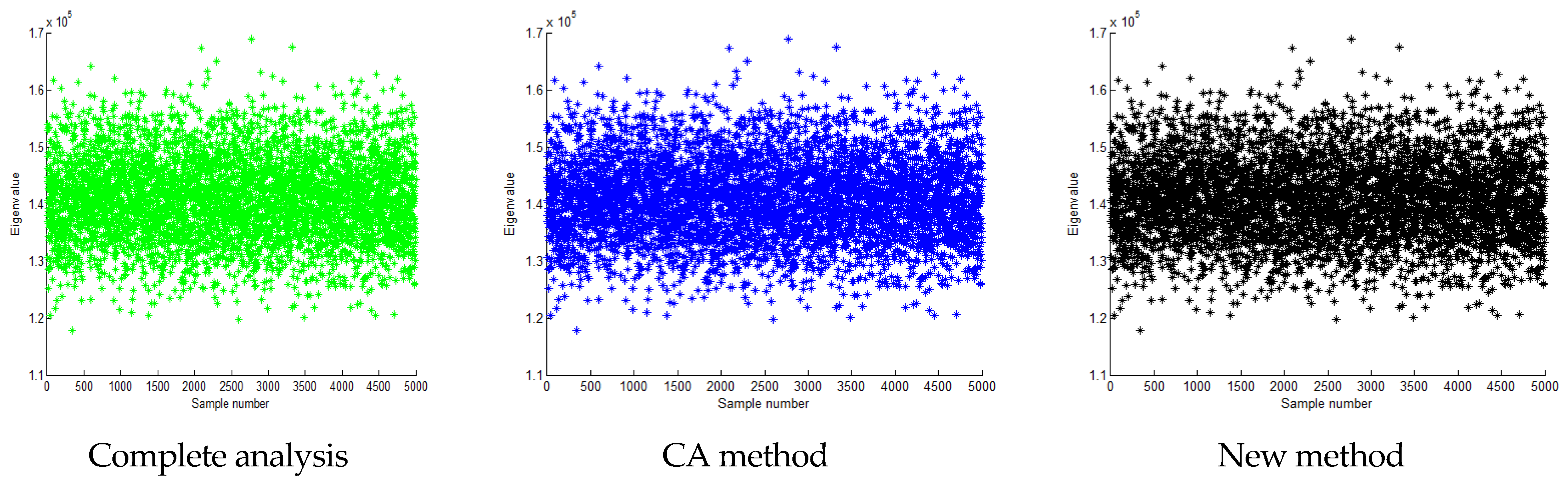
3.1. Example 1: A Truss Structure

A 58-bar structure depicted in Figure 2 was utilized as the example to validate the proposed algorithm. This structure has 51 degrees of freedom (DOFs) and 7 redundant constraints, indicating it is statically indeterminate with a proportion of redundant constraints of about 10% of total members. Each horizontal or vertical rod measures 0.5 m in length, and all members share a cross-sectional area of 314 mm². The density of the material is 7800 kg/m³. It is assumed that the elastic modulus of the material adheres to a normal distribution, with a mean value being assigned as 200 GPa. Within this context, three scenarios for the standard deviation are contemplated: they are determined as 0.1, 0.15, and 0.2 times the mean value, respectively. In a modal stochastic analysis, 5000 random samples were analyzed, and the first three modes post-sampling were computed using the proposed method, the CA reanalysis method [13], and a complete analysis.

For the case where the standard deviation is 0.1 times the mean value, the computation times required for the complete analysis, the CA algorithm, and the new algorithm (with three added basis vectors) are listed in

Table 1. Computation time when the standard deviation is 0.1 times the mean value.

Method	$\mathbf{Complete} \mathbf{Analysis} ({\mathit{t}}_1$)	$\mathbf{CA} \mathbf{Method} ({\mathit{t}}_2$)	$\mathbf{New} \mathbf{Method} ({\mathit{t}}_3$)
Time/s	$t_1$ = 43.53 -- --	$t_2$ = 0.794 $t_2/t_1$ = 1.8% --	$t_3$ = 0.516 $t_3/t_1$ = 1.2% $t_3/t_2$ = 65%

. According to Table 1, the computation times for both the CA and new algorithms are significantly shorter than those of the full analysis. Specifically, the CA algorithm takes approximately 1.8% of the time required by full analysis, whereas the proposed algorithm requires only 1.2% of the full analysis time and 65% of the CA algorithm’s time. Evidently, the proposed method demonstrates the highest level of computational efficiency among the three. Figure 3 presents the first eigenvalues for the 5000 samples calculated by the three methods. As shown in Figure 3, the first-order eigenvalues of each sample calculated by the three methods are concentrated near the median, with a distribution pattern similar to a normal distribution. This indicates that when random sampling is performed for elastic modulus according to a normal distribution, the eigenvalues of the obtained samples also basically follow a normal distribution. The range, mean, and standard deviation of the first eigenvalues are listed in

Table 2. Statistical characteristics of the first eigenvalue when the standard deviation is 0.1 times the mean value.

Method	Complete Analysis	CA Method	New Method
Range (×104)	[1.0222, 1.3519]	[1.0222, 1.3519]	[1.0222, 1.3519]
Mean (×104)	1.1873	1.1873 (0.00%) *	1.1873 (0.00%)
Standard deviation	455.4689	455.4677 (0.00%)	455.4689 (0.00%)

* The data in parentheses indicate the percentage error between the calculated value and the precise value obtained from the complete analysis.

. Note that the results obtained from the complete analysis seem to be the exact solutions for comparison purposes. As can be seen from Table 2, the results obtained by the two rapid algorithms are basically the same as the exact solution. In addition, Figure 4 provides the relative errors of the CA and new methods. The comparative errors of the eigenvalues and eigenvectors are computed by:

$$e_j^{\lambda }={\displaystyle \frac{\left|{\lambda }_j^{calculated}-{\lambda }_j^{exact}\right|}{{\lambda }_j^{exact}}}$$

(44)

$$e_j^{\varphi }={\displaystyle \frac{‖{\varphi }_j^{calculated}-{\varphi }_j^{exact}‖}{‖{\varphi }_j^{exact}‖}}$$

(45)

where $‖\cdot ‖$ represents the two-norm of a vector. As shown in Figure 4, the calculation error of the proposed method is obviously smaller than that of the CA method. Similarly, Figure 5, Figure 6, Figure 7 and Figure 8 and

Table 3. Statistical characteristics of the second eigenvalue when the standard deviation is 0.1 times the mean value.

Method	Complete Analysis	CA Method	New Method
Range (×105)	[1.2779, 1.6027]	[1.2779, 1.6027]	[1.2779, 1.6027]
Mean (×105)	1.4233	1.4233 (0.00%)	1.4233 (0.00%)
Standard deviation	4751.3	4751.3 (0.00%)	4751.3 (0.00%)

and

Table 4. Statistical characteristics of the third eigenvalue when the standard deviation is 0.1 times the mean value.

Method	Complete Analysis	CA Method	New Method
Range (×105)	[6.1859, 7.7367]	[6.1860, 7.7367]	[6.1860, 7.7367]
Mean (×105)	6.8872	6.8873 (0.00%)	6.8873 (0.00%)
Standard deviation	21,122	21,122 (0.00%)	21,122 (0.00%)

present the calculation results for the second and third eigenvalues by the three methods. Figure 5 and Figure 7 show that the second-order and third-order eigenvalues of the samples calculated by the three methods are also concentrated near the median, with a distribution pattern similar to a normal distribution. Figure 6 and Figure 8 show that the calculation errors of the second-order and third-order eigenvalues obtained by the proposed method are also smaller than those of the CA method. It has been shown that the proposed method can achieve higher calculation accuracy than the CA method in less calculation time.

In the scenario where the standard deviation is 0.15 times the mean value,

Table 5. Computation time when the standard deviation is 0.15 times the mean value.

Method	$\mathbf{Complete} \mathbf{Analysis} ({\mathit{t}}_1$)	$\mathbf{CA} \mathbf{Method} ({\mathit{t}}_2$)	$\mathbf{New} \mathbf{Method} ({\mathit{t}}_3$)
Time/s	$t_1$ = 44.163 -- --	$t_2$ = 0.853 $t_2/t_1$ = 1.9% --	$t_3$ = 0.513 $t_3/t_1$ = 1.2% $t_3/t_2$ = 60%

outlines the computation times necessary for the comprehensive analysis, the CA algorithm, and the new algorithm. As evident from Table 5, both the CA and the novel algorithm exhibit substantial reductions in computation time compared to the full analysis. Specifically, the CA algorithm consumes roughly 1.9% of the full analysis’s time, while the proposed algorithm further optimizes, requiring just 1.2% of the full analysis’s duration and 60% of the CA algorithm’s time. Clearly, the proposed method emerges as the most computationally efficient among the three. Figure 9, Figure 10, Figure 11, Figure 12, Figure 13 and Figure 14 and

Table 6. Statistical characteristics of the first eigenvalue when the standard deviation is 0.15 times the mean value.

Method	Complete Analysis	CA Method	New Method
Range (×104)	[0.9264, 1.4296]	[0.9264, 1.4296]	[0.9264, 1.4296]
Mean (×104)	1.1755	1.1755 (0.00%)	1.1755 (0.00%)
Standard deviation	691.9361	691.9117 (0.00%)	691.9361 (0.00%)

,

Table 7. Statistical characteristics of the second eigenvalue when the standard deviation is 0.15 times the mean value.

Method	Complete Analysis	CA Method	New Method
Range (×105)	[1.1772, 1.6882]	[1.1774, 1.6883]	[1.1772, 1.6882]
Mean (×105)	1.4097	1.4097 (0.00%)	1.4097 (0.00%)
Standard deviation	7174.3	7174.0 (0.00%)	7174.3 (0.00%)

and

Table 8. Statistical characteristics of the third eigenvalue when the standard deviation is 0.15 times the mean value.

Method	Complete Analysis	CA Method	New Method
Range (×105)	[5.8076, 8.1225]	[5.8077, 8.1229]	[5.8076, 8.1226]
Mean (×105)	6.8165	6.8167 (0.00%)	6.8166 (0.00%)
Standard deviation	31,844	31,843 (0.00%)	31,844 (0.00%)

display the outcomes of the first, second, and third eigenvalue calculations using these three methods. Figure 9, Figure 11, and Figure 13, respectively, show that the first, second, and third-order eigenvalues of the samples obtained by the three methods are concentrated near the median, resembling a normal distribution. Figure 10, Figure 12, and Figure 14, respectively, show that the calculation errors of the first, second, and third-order eigenvalues obtained by the proposed method are all smaller than those of the CA method. These results demonstrate that the proposed method aligns more closely with the exact solution derived from the full analysis than those of the CA method. This underscores the ability of the proposed method to attain higher calculation accuracy within a shorter computation time compared to the CA method.

In the scenario where the standard deviation is equivalent to 0.2 times the mean value,

Table 9. Computation time when the standard deviation is 0.2 times the mean value.

Method	$\mathbf{Complete} \mathbf{Analysis} ({\mathit{t}}_1$)	$\mathbf{CA} \mathbf{Method} ({\mathit{t}}_2$)	$\mathbf{New} \mathbf{Method} ({\mathit{t}}_3$)
Time/s	$t_1$ = 45.084 -- --	$t_2$ = 0.794 $t_2/t_1$ = 1.8% --	$t_3$ = 0.529 $t_3/t_1$ = 1.2% $t_3/t_2$ = 67%

details the computational time demands for a comprehensive analysis, the CA algorithm, and the innovative algorithm. As evident from Table 9, both the CA algorithm and the novel algorithm exhibit markedly reduced computation times compared to the exhaustive analysis. Precisely, the CA algorithm consumes approximately 1.8% of the time utilized by the full analysis, whereas the presented algorithm requires an even more streamlined 1.2% of the full analysis duration, being 67% as time-consuming as the CA algorithm. Evidently, the proposed method outperforms both in terms of computational efficiency. Additionally, Figure 15, Figure 16, Figure 17, Figure 18, Figure 19 and Figure 20 and

Table 10. Statistical characteristics of the first eigenvalue when the standard deviation is 0.2 times the mean value.

Method	Complete Analysis	CA Method	New Method
Range (×104)	[0.7571, 1.4768]	[0.7582, 1.4769]	[0.7571, 1.4768]
Mean (×104)	1.1577	1.1577 (0.00%)	1.1577 (0.00%)
Standard deviation	963.8251	963.5571 (0.03%)	963.8249 (0.00%)

,

Table 11. Statistical characteristics of the second eigenvalue when the standard deviation is 0.2 times the mean value.

Method	Complete Analysis	CA Method	New Method
Range (×105)	[1.0349, 1.8033]	[1.0359, 1.8035]	[1.0349, 1.8033]
Mean (×105)	1.3884	1.3886 (0.01%)	1.3884 (0.00%)
Standard deviation	9786.9	9782.2 (0.05%)	9786.9 (0.00%)

and

Table 12. Statistical characteristics of the third eigenvalue when the standard deviation is 0.2 times the mean value.

Method	Complete Analysis	CA Method	New Method
Range (×105)	[4.9208, 8.6974]	[4.9642, 8.6985]	[4.9240, 8.6975]
Mean (×105)	6.7002	6.7013 (0.02%)	6.7003 (0.00%)
Standard deviation	42,387	42,353 (0.08%)	42,387 (0.00%)

showcase the eigenvalue computation outcomes for the first, second, and third eigenvalues utilizing these three methodologies. Figure 15, Figure 17, and Figure 19, respectively, illustrate that the first, second, and third-order eigenvalues of the samples, calculated using the three methods, are centered around the median, exhibiting a normal distribution-like pattern. Similarly, Figure 16, Figure 18, and Figure 20 reveal that the calculation errors associated with the first, second, and third-order eigenvalues, respectively, obtained through the proposed method are consistently lower than those obtained via the CA method. The analysis reveals that the calculation error of the proposed method is lower than that of the CA method, with its results aligning more closely with the exact solution derived from the exhaustive analysis. Thus, it is demonstrated that the proposed algorithm achieves higher accuracy while maintaining a shorter computation time compared to the CA method.

According to Table 2, Table 3 and Table 4, Table 6, Table 7 and Table 8, and Table 10, Table 11 and Table 12, the ratios of the standard deviations to the means for the first three eigenvalues calculated by the proposed method are listed in

Table 13. The ratios of the standard deviations to the means for the first three eigenvalues calculated by the proposed method.

Scenario	The Ratios of the Standard Deviations to the Means for the First Three Eigenvalues
	The First Eigenvalue	The Second Eigenvalue	The Third Eigenvalue
The standard deviation of the elastic modulus is 0.1 times the mean value	0.038	0.033	0.031
The standard deviation of the elastic modulus is 0.15 times the mean value	0.059	0.051	0.047
The standard deviation of the elastic modulus is 0.2 times the mean value	0.083	0.070	0.063

. As can be seen from Table 13, as the standard deviation of the elastic modulus increases, the ratio of the standard deviation to the mean of the eigenvalues calculated by the proposed method also gradually increases. In other words, the degree of dispersion of the eigenvalues increases with the increase in the standard deviation of the elastic modulus.

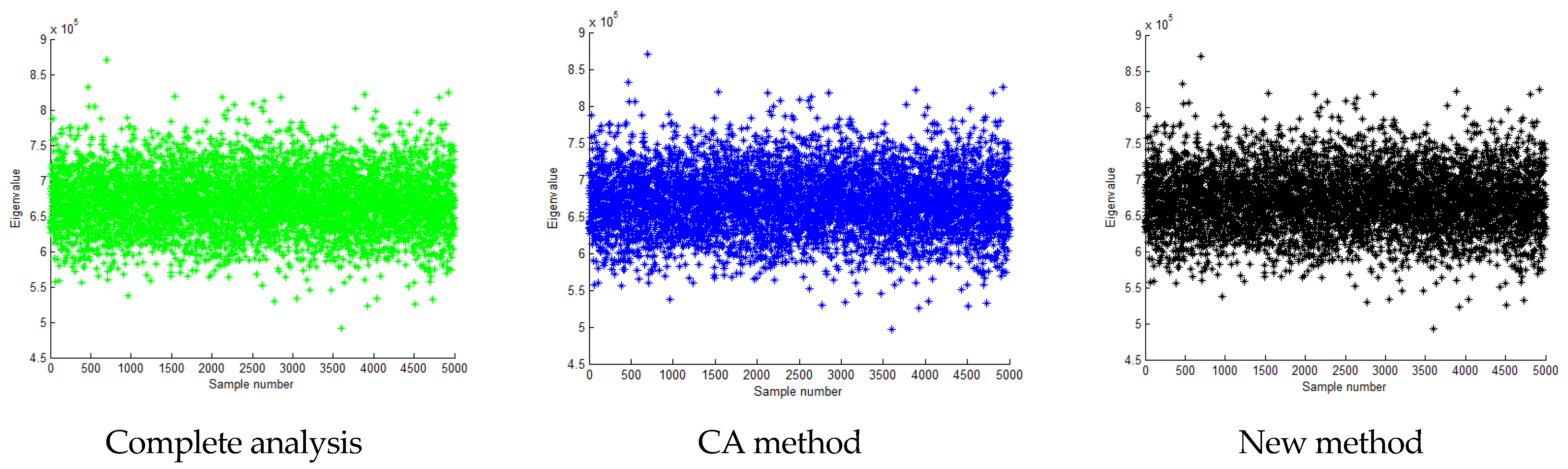
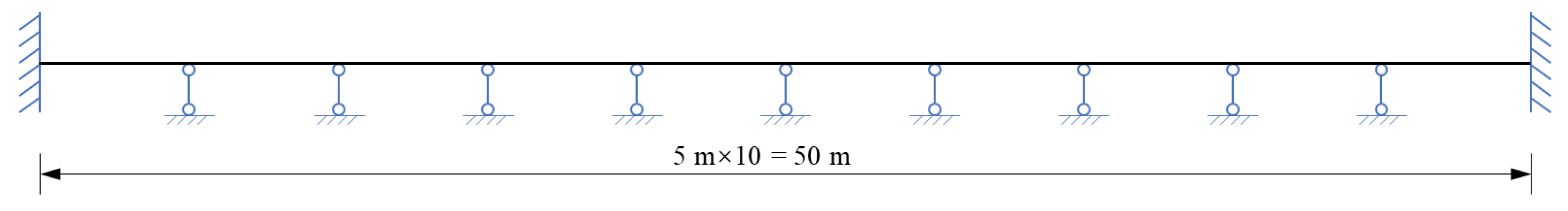
3.2. Example 2: A Beam Structure

The purpose of the second example is to compare the performance of the proposed method with the Ritz vector method [32] in stochastic modal analysis and, additionally, to investigate the computational performance of the proposed method as the number of random variables increases. As shown in Figure 21, this beam structure spans 50 m and is evenly divided into 100 elements. The cross-sectional height of the beam structure is 0.5 m and the width is 0.3 m, with a material density of 2700 kg/m³. Assuming that the elastic moduli follow a normal distribution with a mean of 35 GPa and a standard deviation equal to 0.2 times the mean, the following three sets of samples with different numbers of random variables are examined: the elastic moduli of the first 30 elements are treated as random variables, the elastic moduli of the first 60 elements are treated as random variables, and the elastic moduli of all elements are treated as random variables. During the modal stochastic analysis, 10,000 random samples were examined, and subsequently, the first three modes were calculated using three approaches: the proposed method, the Ritz vector method, and a comprehensive analysis.

Table 14. Computation time for the three sets of samples with different numbers of random variables.

Scenario	$\mathbf{Complete} \mathbf{Analysis} \left({\mathit{t}}_1\right)$	$\mathbf{Ritz} \mathbf{Vector} \mathbf{Method} \left({\mathit{t}}_2\right)$	$\mathbf{New} \mathbf{Method} \left({\mathit{t}}_3\right)$
The elastic moduli of the first 30 elements are treated as random variables	$t_1$ = 198.39 -- --	$t_2$ = 9.10 $t_2/t_1$ = 4.6% --	$t_3$ = 4.42 $t_3/t_1$ = 2.2% $t_3/t_2$ = 48.6%
The elastic moduli of the first 60 elements are treated as random variables	$t_1$ = 200.14 -- --	$t_2$ = 8.83 $t_2/t_1$ = 4.4% --	$t_3$ = 4.35 $t_3/t_1$ = 2.2% $t_3/t_2$ = 49.3%
The elastic moduli of all elements are treated as random variables	$t_1$ = 229.17 -- --	$t_2$ = 9.81 $t_2/t_1$ = 4.3% --	$t_3$ = 4.59 $t_3/t_1$ = 2.0% $t_3/t_2$ = 46.8%

presents a comparison of the computation times for the three methods. From Table 14, the computation times for both the Ritz vector method and the new algorithm are significantly shorter than those of the full analysis. For example, when the elastic modulus of all elements is treated as a random variable, the Ritz vector algorithm takes approximately 4.3% of the time required by the full analysis, whereas the proposed algorithm requires only 2.0% of the full analysis time and 46.8% of the Ritz vector algorithm’s time. On average, the computational time of the proposed method is approximately 2.1% of that required for a full analysis and roughly 48.2% of the Ritz vector method. This demonstrates that the proposed method has the highest computational efficiency. In terms of computational accuracy,

Table 15. Statistical characteristics of the first eigenvalue for example 2 when the elastic moduli of the first 30 elements are treated as random variables.

Method	Complete Analysis	Ritz Vector Method	New Method
Range (×105)	[0.9695, 1.2268]	[0.9702, 1.2268]	[0.9701, 1.2268]
Mean (×105)	1.1919	1.1919 (0.00%) *	1.1919 (0.00%)
Standard deviation	2031.9	2028.3 (0.18%)	2029.2 (0.13%)

* The data in parentheses indicate the percentage error between the calculated value and the precise value obtained from the complete analysis.

,

Table 16. Statistical characteristics of the second eigenvalue for example 2 when the elastic moduli of the first 30 elements are treated as random variables.

Method	Complete Analysis	Ritz Vector Method	New Method
Range (×105)	[1.2651, 1.4406]	[1.2652, 1.4407]	[1.2652, 1.4407]
Mean (×105)	1.3524	1.3524 (0.00%)	1.3524 (0.00%)
Standard deviation	2662.4	2660.8 (0.06%)	2661.2 (0.05%)

,

Table 17. Statistical characteristics of the third eigenvalue for example 2 when the elastic moduli of the first 30 elements are treated as random variables.

Method	Complete Analysis	Ritz Vector Method	New Method
Range (×105)	[1.4802, 1.7036]	[1.4854, 1.7038]	[1.4837, 1.7037]
Mean (×105)	1.5991	1.5992 (0.01%)	1.5992 (0.01%)
Standard deviation	2010.3	2008.0 (0.11%)	2008.6 (0.08%)

,

Table 18. Statistical characteristics of the first eigenvalue for example 2 when the elastic moduli of the first 60 elements are treated as random variables.

Method	Complete Analysis	Ritz Vector Method	New Method
Range (×105)	[0.8629, 1.2717]	[0.8648, 1.2717]	[0.8644, 1.2717]
Mean (×105)	1.1647	1.1648 (0.01%)	1.1648 (0.01%)
Standard deviation	3845.8	3842.1 (0.10%)	3842.9 (0.08%)

,

Table 19. Statistical characteristics of the second eigenvalue for example 2 when the elastic moduli of the first 60 elements are treated as random variables.

Method	Complete Analysis	Ritz Vector Method	New Method
Range (×105)	[1.2080, 1.4541]	[1.2081, 1.4544]	[1.2081, 1.4543]
Mean (×105)	1.3423	1.3424 (0.01%)	1.3424 (0.01%)
Standard deviation	2940.0	2938.2 (0.06%)	2938.9 (0.04%)

,

Table 20. Statistical characteristics of the third eigenvalue for example 2 when the elastic moduli of the first 60 elements are treated as random variables.

Method	Complete Analysis	Ritz Vector Method	New Method
Range (×105)	[1.4252, 1.6981]	[1.4261, 1.6983]	1.4260, 1.6983]
Mean (×105)	1.5773	1.5775 (0.01%)	1.5775 (0.01%)
Standard deviation	3834.7	3830.7 (0.10%)	3831.5 (0.08%)

,

Table 21. Statistical characteristics of the first eigenvalue for example 2 when the elastic moduli of all elements are treated as random variables.

Method	Complete Analysis	Ritz Vector Method	New Method
Range (×105)	[0.8364, 1.2925]	[0.8369, 1.2926]	[0.8369, 1.2926]
Mean (×105)	1.1456	1.1458 (0.02%)	1.1458 (0.02%)
Standard deviation	4203.0	4199.5 (0.08%)	4200.6 (0.06%)

,

Table 22. Statistical characteristics of the second eigenvalue for example 2 when the elastic moduli of all elements are treated as random variables.

Method	Complete Analysis	Ritz Vector Method	New Method
Range (×105)	[1.1000, 1.4688]	[1.1004, 1.4689]	[1.1003, 1.4689]
Mean (×105)	1.3140	1.3143 (0.02%)	1.3142 (0.02%)
Standard deviation	4363.5	4361.5 (0.05%)	4361.9 (0.04%)

and

Table 23. Statistical characteristics of the third eigenvalue for example 2 when the elastic moduli of all elements are treated as random variables.

Method	Complete Analysis	Ritz Vector Method	New Method
Range (×105)	[1.3585, 1.7274]	[1.3589, 1.7277]	[1.3589, 1.7277]
Mean (×105)	1.5523	1.5526 (0.02%)	1.5526 (0.02%)
Standard deviation	4971.5	4969.8 (0.03%)	4970.3 (0.02%)

provide the statistical results of the first three eigenvalues obtained by three methods for the three sets of samples with different numbers of random variables, respectively. As can be seen from Table 15, Table 16, Table 17, Table 18, Table 19, Table 20, Table 21, Table 22 and Table 23, the computational accuracy of the proposed method is also superior to that of the Ritz vector method. According to Table 15, Table 16, Table 17, Table 18, Table 19, Table 20, Table 21, Table 22 and Table 23, the ratios of the standard deviations to the means for the first three eigenvalues calculated by the proposed method are listed in

Table 24. The ratios of the standard deviations to the means for the first three eigenvalues of example 2 calculated by the proposed method.

Scenario	The Ratios of the Standard Deviations to the Means for the First Three Eigenvalues
	The First Eigenvalue	The Second Eigenvalue	The Third Eigenvalue
The elastic moduli of the first 30 elements are treated as random variables	0.017	0.020	0.013
The elastic moduli of the first 60 elements are treated as random variables	0.033	0.022	0.024
The elastic moduli of all elements are treated as random variables	0.037	0.033	0.032

. As can be seen from Table 24, as the number of random variables increases, the ratio of the standard deviation to the mean of the eigenvalues calculated by the proposed method also gradually increases. In other words, the degree of dispersion of the eigenvalues increases with the increase in the number of random variables.

4. Conclusions

This research presents a novel fast algorithm designed to drastically reduce the computational burden associated with modal random analysis of structures. The core concept revolves around enhancing the efficiency of the subspace iteration method through the integration of the FDP technique and the utilization of extended basis vectors. Initially, the FDP formula is employed to swiftly approximate the perturbed flexibility matrix of a random FEM sample characterized by a high number of random variables. Subsequently, this perturbed flexibility matrix is incorporated into the subspace iteration algorithm to promptly extract the perturbed modal parameters of the FEM sample. For statically indeterminate structures, a dedicated formula is introduced to generate additional basis vectors, thereby expanding the subspace and further refining the calculation accuracy. To demonstrate the accuracy and efficiency of the proposed algorithm, a truss structure and a beam structure are analyzed. The comparative study yields the following key insights: (1) The novel modal random analysis algorithm achieves substantial savings in computational time. For the 58-bar structure, the calculation time of the proposed method is approximately 1.2% and 65% of that required by the comprehensive analysis method and the CA method, respectively. For the beam structure, on average, the computational time of the proposed method is approximately 2.1% of that required for a full analysis and roughly 48.2% of the time needed for the Ritz vector method. (2) The results obtained using the proposed method closely approximate the exact solution derived from the comprehensive analysis, demonstrating superior accuracy and efficiency compared to the CA method and Ritz vector method. (3) Notably, the performance of the proposed method remains stable even as the discreteness of structural parameters increases, making it an ideal choice for modal random analysis of highly discrete structures, balancing both computational time and accuracy.

References

1. Men, P.; Wang, X.; Liu, D.; Zhang, Z.; Zhang, Q.; Lu, Y. On use of polyvinylpyrrolidone to modify polyethylene fibers for improving tensile properties of high strength ECC. Constr. Build. Mater. 2024, 417, 135354. [Google Scholar] [CrossRef]
2. Peng, X.; Shi, F.; Yang, J.; Yang, Q.; Wang, H.; Zhang, J. Modification of construction waste derived recycled aggregate via CO2 curing to enhance corrosive freeze-thaw durability of concrete. J. Clean. Prod. 2023, 405, 137016. [Google Scholar] [CrossRef]
3. Zhang, G.Z.; Liu, C.; Cheng, P.F.; Li, Z.; Han, Y.; Wang, X.Y. Enhancing the Interfacial Compatibility and Self-Healing Performance of Microbial Mortars by Nano-SiO2-Modified Basalt Fibers. Cem. Concr. Compos. 2024, 152, 105650. [Google Scholar] [CrossRef]
4. Clough, R.W.; Penzien, J.P. Dynamics of Structures; McGraw–Hill: New York, NY, USA, 1993. [Google Scholar]
5. Bathe, K.J. Finite Element Procedures; Prentice–Hall: Upper Saddle River, NJ, USA, 1996. [Google Scholar]
6. Dong, B.; Parker, R.G. Sector-model subspace iteration for vibration of multi-stage, cyclically symmetric systems. J. Sound Vib. 2023, 544, 117378. [Google Scholar] [CrossRef]
7. Xu, H.; Liu, B. Hierarchical subspace evolution method for super large parallel computing: A linear solver and an eigensolver as examples. Int. J. Numer. Methods Eng. 2023, 124, 5–39. [Google Scholar] [CrossRef]
8. Friswell, M.I.; Garvey, S.D.; Penny, J.E.T. Model reduction using dynamic and iterated IRS techniques. J. Sound Vib. 1995, 186, 311–323. [Google Scholar] [CrossRef]
9. Lin, Y.; Simoncini, V. A new subspace iteration method for the algebraic Riccati equation. Numer. Linear Algebra Appl. 2015, 22, 26–47. [Google Scholar] [CrossRef]
10. Gu, M. Subspace iteration randomization and singular value problems. SIAM J. Sci. Comput. 2015, 37, A1139–A1173. [Google Scholar] [CrossRef]
11. Lasecka-Plura, M.; Lewandowski, R. The subspace iteration method for nonlinear eigenvalue problems occurring in the dynamics of structures with viscoelastic elements. Comput. Struct. 2021, 254, 106571. [Google Scholar] [CrossRef]
12. Chen, S.H.; Yang, X.W.; Lian, H.D. Comparison of several eigenvalue reanalysis methods for modified structures. Struct. Multidiscip. Optim. 2000, 20, 253–259. [Google Scholar]
13. Chen, S.H.; Yang, X.W. Extended Kirsch combined method for eigenvalue reanalysis. AIAA J. 2000, 38, 927–930. [Google Scholar] [CrossRef]
14. Kirsch, U. Approximate vibration reanalysis of structures. AIAA J. 2003, 41, 504–511. [Google Scholar] [CrossRef]
15. Kirsch, U.; Bogomolni, M. Procedures for approximate eigenproblem reanalysis of structures. Int. J. Numer. Methods Eng. 2004, 60, 1969–1986. [Google Scholar] [CrossRef]
16. Yang, Z.J.; Chen, S.H.; Wu, X.M. A method for modal reanalysis of topological modifications of structures. Int. J. Numer. Methods Eng. 2006, 65, 2203–2220. [Google Scholar] [CrossRef]
17. Hong, S.-K.; Epureanu, B.I.; Castanier, M.P.; Gorsich, D.J. Parametric reduced-order models for predicting the vibration response of complex structures with component damage and uncertainties. J. Sound Vib. 2011, 330, 1091–1110. [Google Scholar] [CrossRef]
18. Xu, T.; Guo, G.; Zhang, H. Vibration reanalysis using frequency-shift combined approximations. Struct. Multidiscip. Optim. 2011, 44, 235–246. [Google Scholar] [CrossRef]
19. Norouzi, M.; Nikolaidis, E. Efficient method for reliability assessment under high-cycle fatigue. Int. J. Reliab. Qual. Saf. Eng. 2012, 19, 1250022. [Google Scholar] [CrossRef]
20. Mourelatos, Z.P.; Nikolaidis, E. An efficient re-analysis methodology for vibration of large-scale structures. Int. J. Veh. Des. 2013, 61, 86–107. [Google Scholar] [CrossRef]
21. Zheng, S.P.; Wu, B.S.; Li, Z.G. Vibration reanalysis based on block combined approximations with shifting. Comput. Struct. 2015, 149, 72–80. [Google Scholar] [CrossRef]
22. Liu, H.; Wang, H.; Tan, G.; Liu, Z. Reanalysis of the structural dynamic characteristics based on double coordinate free-interface mode synthesis & matrix perturbation method. Vibroengineering Procedia 2016, 10, 83–88. [Google Scholar]
23. Li, D.; Zhou, Q.; Chen, G.; Li, Y. Structural dynamic reanalysis method for transonic aeroelastic analysis with global structural modifications. J. Fluids Struct. 2017, 74, 306–320. [Google Scholar] [CrossRef]
24. Zheng, S.P.; Wu, B.S.; Li, Z.G. Free vibration reanalysis of structures with added degrees of freedom. Comput. Struct. 2018, 206, 31–41. [Google Scholar] [CrossRef]
25. Huang, G.; Chen, X.; Yang, Z.; Wu, B. Exact analysis and reanalysis methods for structures with nonlinear boundary conditions. Comput. Struct. 2018, 198, 12–22. [Google Scholar] [CrossRef]
26. He, J.; Chen, X.; Xu, B. Structural modal reanalysis for large, simultaneous and multiple type modifications. Mech. Syst. Signal Process. 2015, 62, 207–217. [Google Scholar]
27. He, J.; Xu, B. Quick and Highly Efficient Modal Analysis Method Based on the Reanalysis Technique for Large Complex Structure and Topology Optimization. Int. J. Comput. Methods 2020, 17, 1850134. [Google Scholar] [CrossRef]
28. Chang, S.; Cho, M. Dynamic-condensation-based reanalysis by using the Sherman–Morrison–Woodbury formula. AIAA J. 2021, 59, 905–911. [Google Scholar] [CrossRef]
29. Li, W.; Chen, S. An improved model order reduction method for dynamic analysis of large-scale structures with local nonlinearities. Appl. Math. Model. 2023, 120, 786–811. [Google Scholar] [CrossRef]
30. Yang, Q.W. Fast and Exact Algorithm for Structural Static Reanalysis Based on Flexibility Disassembly Perturbation. AIAA J. 2019, 57, 3599–3607. [Google Scholar] [CrossRef]
31. Yang, Q.W.; Peng, X. A Fast Calculation Method for Sensitivity Analysis Using Matrix Decomposition Technique. Axioms 2023, 12, 179. [Google Scholar] [CrossRef]
32. Koh, H.S.; Yoon, G.H. Ritz vector-based substructuring method using interface eigenmode-shape pseudo-forces. Finite Elem. Anal. Des. 2023, 227, 104023. [Google Scholar] [CrossRef]
Figure 1. The operation flow of the proposed algorithm for random modal analysis of statically indeterminate structures.
Mathematics 12 03486 g001
Figure 2. A truss structure with 58 rods.
Mathematics 12 03486 g002
Figure 3. Calculation result of the first eigenvalue when the standard deviation is 0.1 times the mean value.
Mathematics 12 03486 g003
Figure 4. Calculation errors of the first eigen-pairs when the standard deviation is 0.1 times the mean value.
Mathematics 12 03486 g004
Figure 5. Calculation result of the second eigenvalue when the standard deviation is 0.1 times the mean value.
Mathematics 12 03486 g005
Figure 6. Calculation errors of the second eigen-pairs when the standard deviation is 0.1 times the mean value.
Mathematics 12 03486 g006
Figure 7. Calculation result of the third eigenvalue when the standard deviation is 0.1 times the mean value.
Mathematics 12 03486 g007
Figure 8. Calculation errors of the third eigen-pairs when the standard deviation is 0.1 times the mean value.
Mathematics 12 03486 g008
Figure 9. Calculation result of the first eigenvalue when the standard deviation is 0.15 times the mean value.
Mathematics 12 03486 g009
Figure 10. Calculation errors of the first eigen-pairs when the standard deviation is 0.15 times the mean value.
Mathematics 12 03486 g010
Figure 11. Calculation result of the second eigenvalue when the standard deviation is 0.15 times the mean value.
Mathematics 12 03486 g011
Figure 12. Calculation errors of the second eigen-pairs when the standard deviation is 0.15 times the mean value.
Mathematics 12 03486 g012
Figure 13. Calculation result of the third eigenvalue when the standard deviation is 0.15 times the mean value.
Mathematics 12 03486 g013
Figure 14. Calculation errors of the third eigen-pairs when the standard deviation is 0.15 times the mean value.
Mathematics 12 03486 g014
Figure 15. Calculation result of the first eigenvalue when the standard deviation is 0.2 times the mean value.
Mathematics 12 03486 g015
Figure 16. Calculation errors of the first eigen-pairs when the standard deviation is 0.2 times the mean value.
Mathematics 12 03486 g016
Figure 17. Calculation result of the second eigenvalue when the standard deviation is 0.2 times the mean value.
Mathematics 12 03486 g017
Figure 18. Calculation errors of the second eigen-pairs when the standard deviation is 0.2 times the mean value.
Mathematics 12 03486 g018
Figure 19. Calculation result of the third eigenvalue when the standard deviation is 0.2 times the mean value.
Mathematics 12 03486 g019
Figure 20. Calculation errors of the third eigen-pairs when the standard deviation is 0.2 times the mean value.
Mathematics 12 03486 g020
Figure 21. A beam structure.
Mathematics 12 03486 g021