Article

Large Sample Behavior of the Least Trimmed Squares Estimator

Department of Statistics and Probability, Michigan State University, East Lansing, MI 48824, USA
Mathematics 2024, 12(22), 3586; https://doi.org/10.3390/math12223586
Submission received: 30 September 2024 / Revised: 8 November 2024 / Accepted: 11 November 2024 / Published: 15 November 2024
(This article belongs to the Special Issue Advances in High-Dimensional Data Analysis)

Abstract

:
The least trimmed squares (LTS) estimator is popular in location, regression, machine learning, and AI literature. Despite the empirical version of least trimmed squares (LTS) being repeatedly studied in the literature, the population version of the LTS has never been introduced and studied. The lack of the population version hinders the study of the large sample properties of the LTS utilizing the empirical process theory. Novel properties of the objective function in both empirical and population settings of the LTS and other properties, are established for the first time in this article. The primary properties of the objective function facilitate the establishment of other original results, including the influence function and Fisher consistency. The strong consistency is established with the help of a generalized Glivenko–Cantelli Theorem over a class of functions for the first time. Differentiability and stochastic equicontinuity promote the establishment of asymptotic normality with a concise and novel approach.

1. Introduction

In classical multiple linear regression analysis, it is assumed that there is a relationship for a given data set { ( x i , y i ) , i { 1 , , n } } :
y i = ( 1 , x i ) β 0 + e i , i { 1 , , n } ,
where y i and e i (an error term, a random variable, and is assumed to have a zero mean and unknown variance σ 2 in the classic regression theory) are in R 1 , ⊤ stands for the transpose, β 0 = ( β 01 , , β 0 p ) , the true unknown parameter, and x i = ( x i 1 , , x i ( p 1 ) ) is in R p 1 ( p 2 ) and could be random. It is seen that β 01 is the intercept term. Writing w i = ( 1 , x i ) , one has y i = w i β 0 + e i . The classic assumptions such as linearity and homoscedasticity are implicitly assumed here. Others will be considered later when they are needed.
The goal is to estimate the β 0 based on the given sample z ( n ) : = { ( x i , y i ) , i { 1 , , n } } (hereafter, it is implicitly assumed that they are i.i.d. from parent ( x , y ) ). For a candidate coefficient vector β , call the difference between y i (observed) and w i β (predicted), the ith residual, r i ( β ) , ( β is often suppressed). That is,
r i : = r i ( β ) = y i w i β .
To estimate β 0 , the classic least squares (LS) minimizes the sum of squares of residuals,
β ^ l s : = arg min β R p i = 1 n r i 2 .
Alternatively, one can replace the square above with the absolute value to obtain the least absolute deviations estimator (aka, L 1 estimator, in contrast to the L 2 (LS) estimator).
Due to its great computability and optimal properties when the error e i follows a Gaussian distribution, the LS estimator is popular in practice across multiple disciplines. It, however, can misbehave when the error distribution slightly departs from the Gaussian assumption, particularly when the errors are heavy-tailed or contain outliers. Both L 1 and L 2 estimators have the worst 0 % asymptotic breakdown point, in sharp contrast to the 50 % of the least trimmed squares estimator [1]. The latter is one of the most robust alternatives to the LS estimator. Robust alternatives to the LS estimator are abundant in the literature. The most popular are M-estimators [2]), least median squares (LMS) and least trimmed squares (LTS) estimators [3]), S-estimators [4]), MM-estimators [5]), τ -estimators [6]) and maximum depth estimators [7,8,9]), among others.
Although the M-estimator is the first robust alternative to the LS estimator, it has a poor breakdown point, 1 / n , just as the LS whereas the MM-estimator could have a higher breakdown point but it depends on the initial estimator, which must have a high breakdown robustness such as the LTS. So the MM-estimator can have a better efficiency than the LTS but not robustness.
Due to the cube-root consistency of LMS in R84 and its other drawbacks, LTS is preferred over LMS (see [10]). LTS is popular in the literature in view of its fast computability and high robustness and often serves as the initial estimator for many high breakdown iterative procedures (e.g., S- and MM- estimators). The LTS is defined as the minimizer of the sum of h trimmed squares of residuals. Namely,
β ^ l t s : = arg min β R p i = 1 h r i : n 2 ,
where r 1 : n 2 r 2 : n 2 r n : n 2 are the ordered squared residuals and n / 2 h < n and x is the ceiling function.
There are copious studies on the LTS in the literature. Most are focused on its computation, e.g., [1,10,11,12,13,14,15,16,17,18];
The LTS has been extended to penalized regression setting with a sparse model where dimension p (in thousands) is much larger than sample size n (in tens, or hundreds), see, e.g., [19,20]. The resulting estimator performs outstanding, especially in terms of robustness.
Other studies on LTS sporadically addressed the asymptotics, e.g., Refs. [1,21] addressed the asymptotic normality of the LTS, but limited to the location case, that is, when p = 1 . Refs. [22,23,24] also addressed the asymptotics of the LTS without employing advanced technical tools in a series (three) of lengthy articles for consistency, root-n consistency, and asymptotic normality, respectively. The analysis is technically demanding and with difficult-to-verify assumptions A , B , C . Furthermore, the analysis is limited to the non-random vector x i s case. In this article, without those assumptions and limitations, those results are established concisely with the help of advanced empirical process theory.
Replacing ( 1 , x i ) β 0 by a unspecified nonlinear function h ( x i , β 0 ) , Refs. [25,26,27] discussed the asymptotics of the LTS in a nonlinear regression setting. Now that the more general non-linear case has been addressed, one might wonder if there are any merits to discussing the special linear case in this article.
There are at least three merits: (i) the nonlinear function h ( x i , β 0 ) cannot always cover the linear case of ( 1 , x i ) β 0 for the usual LTS (e.g., in the exponential and power regression cases); (ii) many assumptions for the nonlinear case (see A1, A2, A3, A4 in [25]; H1, H2, H3, H4, H5, H6; D1, D2; I1, I2 in [26,27]) (which are usually difficult to verify) can be dropped for the linear case as demonstrated in this article. (iii) A key assumption that { h ( x , β ) , β Θ } form a VC class of functions over a compact parameter space Θ (see [25,26,27]) can be verified directly in this article.
To avoid all the drawbacks and limitations discussed above and take advantage of the standard results of the empirical process theory, this article defines the population version of the LTS (Section 2.1), introduces the novel partition of the parameter space (Section 2.2), and investigates the primary properties of the objective function for the LTS both in the empirical and population settings (Section 2) for the first time. The obtained novel results facilitate the versification of some fundamental assumptions conveniently made previously in the literature. The major contributions of this article thus include the following
(a)
Introducing a novel partition of the parameter space and defining an original population version of the LTS for the first time;
(b)
Investigating primary properties of the sample and population versions of the objective function for the LTS, obtaining original results;
(c)
For the first time, obtaining the influence function ( p 2 ) and Fisher consistency for the LTS;
(d)
For the first time, establishing the strong consistency of the sample LTS via a generalized Glivenko-Cantelli Theorem without artificial assumptions; and
(e)
For the first time, employing a novel and concise approach based on the empirical process theory to establish the asymptotic normality of the sample LTS.
The rest of the article is organized as follows. Section 2 introduces for the first time, the population version of LTS and addresses the properties of the LTS estimator in both empirical and population settings, including the global continuity and local differentiability and convexity of its objective function; its influence function (in p > 2 cases) and Fisher consistency are established for the first time. Section 3 establishes the strong consistency via a generalized Glivenko–Cantelli Theorem and the asymptotic normality of the estimator is re-established in a very different and concise approach (via stochastic equicontinuity) rather than the previous approaches in the literature. Section 4 addresses the asymptotic inference procedures based on the asymptotic normality and bootstrapping. Concluding remarks in Section 5 end the article. Major proofs are deferred to Appendix A.

2. Definition and Properties of the LTS

2.1. Definition

Denote by F ( x , y ) the joint distribution of x and y in model (1). Throughout, F Z stands for the distribution function of the random vector Z . For a given β R p and an α [ 1 / 2 , c ] , 1 / 2 < c < 1 , let q ( β , α ) = F W 1 ( α ) be the α th quantile of F W with W : = W ( β ) = ( y w β ) 2 , where w = ( 1 , x ) . The constant c = 1 case is excluded to avoid unbounded q ( β , α ) and the LS cases. Define an objective function
O ( F ( x , y ) , β , α ) = ( y ( 1 , x ) β ) 2 1 ( y ( 1 , x ) β ) 2 q ( β , α ) d F ( x , y ) ( x , y ) ,
and a regression functional
β l t s ( F ( x , y ) , α ) = arg min β R p O ( F ( x , y ) , β , α ) ,
where 1 ( A ) is the indicator of A (i.e., it is one if A holds and zero otherwise). Let F ( x , y ) n be the sample version of the F ( x , y ) based on a sample z ( n ) : = { ( x i , y i ) , i { 1 , 2 , , n } } . F ( x , y ) n and z ( n ) will be used interchangeably. Using F ( x , y ) n , one obtains the sample versions
O ( F ( x , y ) n , β , α ) = 1 n i = 1 α n + 1 r i : n 2 ,
where x is the floor function. Further
β ^ l t s n : = β l t s ( F ( x , y ) n , α ) = arg min β R p O ( F ( x , y ) n , β , α ) .
It is readily seen that the β ^ l t s n above is identical to the β ^ l t s in (3) with h = α n + 1 . Henceforth, we prefer to treat the β ^ l t s n rather than the β ^ l t s in (3).
The first natural question is the existence of the minimizer in the right-hand side (RHS) of (7), or the existence of the β ^ l t s n . Does it always exist? If it exists, will it be unique? Unique existence is a key precondition for the study of asymptotics of an estimator.
One might take the existence for granted since the objective is non-negative and has a finite infimum that can be approximated by objective values of a sequence of β s. There is a sub-sequence of β s with its objective values converging to the infimum that is a minimum due to the continuity of the objective function. The sub-sequence of β s converges to a point β * , which is the minimizer of the RHS. However, there are multiple issues with the arguments above. The existence and the convergence of the β sub-sequence (to a minimum) and continuity of objective function need to be proved. In the sequel, we take a different approach.

2.2. Properties in the Empirical Case

Write O n ( β ) and 1 i for the O ( F ( x , y ) n , β , α ) and the 1 r i 2 r h : n 2 , respectively. It is seen that
O n ( β ) = 1 n i = 1 n r i 2 1 r i 2 r h : n 2 = 1 n i = 1 n r i 2 1 i ,
where h = α n + 1 . The fraction 1 / n will often be ignored in the following discussion.
  • Existence and uniqueness
  • Partition parameter space
For a given sample z ( n ) , an α (or h), and any β 1 R p , let r i : n 2 ( β 1 ) = r k i 2 ( β 1 ) for an integer k i . Note that r j and k i depend on β 1 , i.e., r j : = r j ( β 1 ) , k i : = k i ( β 1 ) . Obviously r k 1 2 r k 2 2 r k n 2 . Call { k i , 1 i h }   β 1 -h-integer set. If r i 2 r j 2 for any distinct i and j, then the h-integer set is unique. Hereafter, we assume (A0):  W  has a density for any given  β . Then, almost surely (a.s.), the h-integer set is unique.
Consider the unique cases. There are other β s in R p that share the same h-integer set as that of the β 1 . Denote the set of such points that have the same h integers as β 1 by
S β 1 : = β R p : k i ( β ) = k i ( β 1 ) = k i , i { 1 , 2 , , h } { k i , 1 i h } is unique .
If (A0) holds, then S β 1 (a.s.). If it is R p , then we have a trivial case (see Remark 1 below). Otherwise, there are only finitely many such sets (for a fixed n) that partition R p . Let l = 1 L S ¯ β l = R p , where S β l s are defined similarly to (9) and are disjoint for different l, 1 l L : = n h , and A ¯ is the closure of the set A. Write X n = ( w 1 , , w n ) , an n × p matrix. Assume (A1): X n and any its h rows have a full rank p . As in the R function ltsReg in the R package robustbase version 99-4-1, hereafter, we assume that p < n / 2 .
Lemma 1.
Assume that (A0) and (A1) hold, then
(i) 
(a) For any l ( 1 l L ), r k 1 ( β l ) 2 < r k 2 ( β l ) 2 < < r k h ( β l ) 2 over S β l .
(b) For any η S β l , there exists an open ball B ( η , δ ) centered at η with a radius δ > 0 such that for any β B ( η , δ )
O n ( β ) = 1 n i = 1 h r k i ( β ) 2 ( β ) = 1 n i = 1 h r k i ( η ) 2 ( β ) = 1 n i = 1 h r k i ( β l ) 2 ( β ) , ( a . s . )
(ii) 
The graph of O n ( β ) over β R p is composed of the L closures of graphs of the quadratic function of β: 1 n i = 1 h r k i ( β l ) 2 ( β ) for O n ( β l ) and any l ( 1 l L ), joined together.
(iii) 
O n ( β ) is continuous in β R p .
(iv) 
O n ( β ) is differentiable and strictly convex over each S β l for any 1 l L .
Proof. 
See the Appendix A. □
Remark 1.
(a) If S β 0 = R p , then O n ( β ) is a twice differentiable and strictly convex quadratic function of β, the existence and the uniqueness of β ^ l t s n are trivial as long as X n has a full rank.
(b) Replacing ( 1 , x i ) β by a nonlinear h ( x i , β ) , conveniently assuming that (i) F W is twice differentiable around the points corresponding to the square roots of the α-quantiles of W, (ii) h ( x i , β ) is continuous over parameter space B, (iii) h ( x i , β ) is twice differentiable in β for β B ( β 0 , δ ) a.s., and (iv) h ( x i , β ) / β is continuous in β, Refs. [26,27] also addressed the continuity and differentiability of the objective function of the LTS. All assumptions were never verified in [26,27], though; however, they are proved (or not required) in Lemma 1.
(c) Continuity and differentiability inferred just based on O n ( β ) being the sum of h continuous and differentiable functions (squares of residual) without (i) or (10) might not be flawless. In general, O n ( β ) is not differentiable nor convex in β globally.
Let y n : = ( y 1 , , y n ) , M n : = M ( y n , X n , β , α ) = i = 1 n w i w i 1 i = i = 1 h w k i ( β ) w k i ( β ) . Note that 1 i depends on β .
Theorem 1.
Assume that (A0) and (A1) hold. Then,
(i) 
β ^ l t s n exists and is the local minimum of O n ( β ) over S β l 0 for some l 0 ( 1 l 0 L ).
(ii) 
Over S β l 0 , β ^ l t s n is the solution of the system of equations
i = 1 n ( y i w i β ) w i 1 i = 0 ,
(iii) 
Over S β l 0 , the unique solution is
β ^ l t s n = M n ( y n , X n , β ^ l t s n , α ) 1 i = 1 h y k i ( β l 0 ) w k i ( β l 0 ) .
Proof. 
The given conditions and Lemma 1 allow one to focus on a piece S β l , 1 l L , all results follow in a straightforward fashion. For more details, see Appendix A. □
Remark 2.
(a) Unique existence, which is often implicitly assumed or ignored in the literature, is central for the discussion of asymptotics of β ^ l t s n . Existence of β ^ l t s n could also be established under the assumption that there are no ( n + 1 ) / 2 sample points of z ( n ) contained in any ( p 1 ) -dimensional hyperplane, similarly to that of Theorem 2.2 for LST in [28]. It is established here without such an assumption nevertheless.
(b) A sufficient condition for the invertibility of M n is that any h rows of X n form a full rank sub-matrix. The latter is true if (A1) holds.
(c) Ref. [22] also addressed the existence of  β ^ l t s n (Assertion 1) for non-random covariates (carriers) satisfying many demanding assumptions ( A , B ) that are never verified. The uniqueness was left unaddressed, though.

2.3. Properties in the Population Case

The best breakdown point of the LTS (see p. 132 of [1]) reflects its global robustness. We now examine its local robustness via the influence function to depict its complete robust picture.

2.3.1. Definition of Influence Function

For a distribution F on R p and an ε ( 0 , 1 / 2 ) , the version of F contaminated by an ε amount of an arbitrary distribution G on R p is denoted by F ( ε , G ) = ( 1 ε ) F + ε G (an ε amount deviation from the assumed F). F ( ε , G ) is actually a convex contamination of F. There are other types of contamination such as contamination by total variation or Hellinger distances. We cite the definition given in [29].
Definition 1
([29]). The influence function (IF) of a functional t at a given point x R p for a given F is defined as
IF ( x ; t , F ) = lim ε 0 + t ( F ( ε , δ x ) ) t ( F ) ε ,
where δ x is the point-mass probability measure at x R p .
The function IF ( x ; t , F ) describes the relative effect (influence) on t of an infinitesimal point-mass contamination at x and measures the local robustness of t .
To establish the IF for the functional β l t s ( F ( x , y ) , α ) , we need to first show its existence and uniqueness with or without point-mass contamination. To that end, write
F ε ( z ) : = F ( ε , δ z ) = ( 1 ε ) F ( x , y ) + ε δ z ,
with u = ( s , t ) R p , s R p 1 , t R 1 as the corresponding random vector (i.e., F u = F ε ( z ) = F ( ε , δ z ) ). The versions of (4) and (5) at the contaminated F ( ε , δ z ) are, respectively,
O ( F ε ( z ) , β , α ) = ( t ( 1 , s ) β ) 2 1 ( t ( 1 , s ) β ) 2 q ε ( z , β , α ) d F u ( s , t ) ,
with q ε ( z , β , α ) being the α th quantile of the distribution function of ( t v β ) 2 , v = ( 1 , s ) , and
β l t s ( F ε ( z ) , α ) = arg min β R p O ( F ε ( z ) , β , α ) .
For β l t s ( F ( x , y ) , α ) defined in (5) and β l t s ( F ε ( z ) , α ) above, we have an analogous result to Theorem 1. (Assume that the counterpart of model (1) is y = ( 1 , x ) β 0 + e = w β 0 + e ). Before we derive the influence function, we need to establish existence and uniqueness.

2.3.2. Existence and Uniqueness

Write O ( β ) for O ( F ( x , y ) , β , α ) in (4). To have a counterpart of Lemma 1, we need (A2): W has a positive density around a small neighborhood of q ( β , α ) for the given α , β .
Lemma 2.
Assume (A2) holds and E ( w w ) exists. Then,
(i)  O ( β ) is continuous in β R p ;
(ii)  O ( β ) is twice differentiable in β R p ,
2 O ( β ) / β 2 = 2 E ( w w 1 ( ( y w β ) 2 q ( β , α ) ) ) ;
(iii)  O ( β ) is strictly convex in β R p .
Proof. 
The boundedness of the integrand in (4), given conditions, and the Lebesgue-dominated convergence theorem leads to the desired results. For the details, see Appendix A. □
Note that (ii) and (iii) above are global in β , stronger than the empirical counterparts, and all are attributed to the boundary of S β l issue. We now treat the existence and uniqueness of β l t s , which is central to the study of the asymptotics.
Theorem 2.
Assume (A2) holds and E ( w w ) exists, q ε ( z , β , α ) is continuous in β, and P ( ( t v β ) 2 = q ε ( z , β , α ) ) = 0 for any β R p and the given α. Then,
(i)  β l t s ( F ( x , y ) , α ) and β l t s ( F ε ( z ) , α ) exist.
(ii) Furthermore, they are the solution of a system of equations, respectively,
( y ( 1 , x ) β ) ( 1 , x ) 1 ( y ( 1 , x ) β ) 2 q ( β , α ) d F ( x , y ) ( x , y ) = 0 ,
( t ( 1 , s ) β ) ( 1 , s ) 1 ( t ( 1 , s ) β ) 2 q ε ( z , β , α ) d F u ( s , t ) = 0 .
(iii)  β l t s ( F ( x , y ) , α ) and β l t s ( F ε ( z ) , α ) are unique provided that
( 1 , x ) ( 1 , x ) 1 ( y ( 1 , x ) β ) 2 q ( β , α ) d F ( x , y ) ( x , y ) ,
( 1 , s ) ( 1 , s ) 1 ( t ( 1 , s ) β ) 2 q ε ( z , β , α ) d F u ( s , t )
are invertible for β in a small neighborhood of β l t s ( F ( x , y ) , α ) and β l t s ( F ε ( z ) , α ) , respectively.
Proof. 
In light of Lemma 2, the proof is straightforward, see Appendix A. □
The continuity of q ε ( z , β , α ) in β is necessary for the differentiability of O ( F ε ( z ) , β , α ) . In the non-contaminated case, the continuity of q ( β , α ) is guaranteed by (A2).
Does the population version of the LTS, β l t s , defined in (5), have something to do with β 0 ? It turns out that under some conditions, they are identical, which is called Fisher consistency.

2.3.3. Fisher Consistency

Theorem 3.
Assume (A2) holds and E ( w w ) exists, then, β l t s ( F ( x , y ) , α ) = β 0 provided that
(i) 
E ( x , y ) w w 1 ( r ( β ) 2 F r ( β ) 2 1 ( α ) )  is invertible, and
(ii) 
E ( x , y ) ( e w 1 ( e 2 F e 2 1 ( α ) ) ) = 0 , where r ( β ) = y w β .
Proof. 
Theorem 2 leads directly to the desired result, see the Appendix A. □

2.3.4. Influence Function

Theorem 4.
Assume that the assumptions in Theorem 2 hold. Set β l t s : = β l t s ( F ( x , y ) , α ) . Then, for any z 0 : = ( s 0 , t 0 ) R p , we have that
I F ( z 0 ; β l t s , F ( x , y ) ) = 0 , i f ( t 0 v 0 β l t s ) 2 > q ( β l t s , α ) , M 1 ( t 0 v 0 β l t s ) v 0 , o t h e r w i s e ,
provided that M = E ( x , y ) w w 1 r ( β l t s ) 2 q ( β l t s , α ) is invertible, where v 0 = ( 1 , s 0 ) .
Proof. 
The connection to the derivative of a functional is the key, see Appendix A. □
Remark 3.
(a) When p = 1 , the problem in our model (1) becomes a location problem (see p. 158 of [1]) and the IF of the LTS estimation functional is given on p. 191 of [1]. In the location setting, Ref. [30] also studied the IF of the LTS. When p = 2 , namely in the simple regression case, Ref. [31] studied IF of the sparse-LTS functional under the assumption that x and e are independent and normally distributed. Under stringent assumptions on the error terms e i and on x , Ref. [21] also addressed the IF of LTS for any p, but the point mass at ( x , z ) with z being the error term, an unusual contaminating point. The above result is much more general and valid for any p 1 , x , and e.
(b) The influence function of β l t s remains bounded if the contaminating point ( s 0 , t 0 ) does not follow the model (i.e., its residual is extremely large), in particular for bad leverage points and vertical outliers. This shows the good robust properties of the LTS.
(c) The influence function of β l t s , unfortunately, might be unbounded (in p > 1 case), sharing the drawback of the sparse-LTS (in the p = 2 case). The latter was shown in [31]. Trimming based on the residuals (or squared residuals) will have this type of drawback since the term w β can be bounded, but x might not.

3. Asymptotic Properties

Refs. [22,23,24] rigorously addressed the consistency, root-n consistency, and normality of the LTS under a restrictive setting ( x i s are non-random covariates) plus many assumptions on x i s and on the distribution of e i in a series of three lengthy papers.
Refs. [26,27] also addressed asymptotic properties of an extended LTS under β -mixing conditions for x i with nonlinear regression function h ( x i , β ) , a seemingly more general setting, but with numerous artificial assumptions (H1, H2, H3, H4, H5, H6; D1, D2; I1, I2) that are never verified in any concrete example and not even for the linear LTS case. That is, Refs. [26,27] do not cover the LTS in (3).
Here, we address asymptotic properties of β ^ l t s n without the artificial assumptions that were made in the literature for LTS with a nonlinear regression function. Strong consistency has been addressed in [25] in a nonlinear setting without verifying any of their conveniently assumed key assumptions for the linear LTS. We now rigorously establish strong consistency.

3.1. Strong Consistency

Following the notations of [32], write
O ( β , P ) : = O ( F ( x , y ) , β , α ) = P [ ( y w β ) 2 1 ( r ( β ) 2 F r ( β ) 2 1 ( α ) ) ] = P f , O ( β , P n ) : = O ( F ( x , y ) n , β , α ) = 1 n i = 1 n r i 2 1 r i 2 ( r ) h : n 2 = P n f ,
where f : = f ( x , y , β , α ) = ( y w β ) 2 1 ( r ( β ) 2 F r ( β ) 2 1 ( α ) ) , α and h = α n + 1 are fixed.
Under corresponding assumptions in Theorems 1 and 2, β ^ l t s n and β l t s are unique minimizers of O ( β , P n ) and O ( β , P ) , respectively.
To show that β ^ l t s n converges to β l t s a.s., one can take the approach given in Section 4.2 of [28]. However, here, we take a different and more direct approach.
To show that β ^ l t s n converges to β l t s a.s., it will suffice to prove that O ( β ^ l t s n , P ) O ( β l t s , P ) a.s., because O ( β , P ) is bounded away from O ( β l t s , P ) outside each neighborhood of β l t s in light of continuity and compactness. Let Θ be a closed ball centered at β l t s with a radius r > 0 . Define a class of functions
F ( β , α ) = f ( x , y , β , α ) = ( y w β ) 2 1 ( r ( β ) 2 F r ( β ) 2 1 ( α ) ) : β Θ , α [ 1 / 2 , c ]
If we prove uniform almost sure convergence of P n to P over F (see Lemma 3 below), then we can deduce that O ( β ^ l t s n , P ) O ( β l t s , P ) a.s. from
O ( β ^ l t s n , P n ) O ( β ^ l t s n , P ) 0 ( in   light   of   Lemma   3 ) , and O ( β ^ l t s n , P n ) O ( β l t s , P n ) O ( β l t s , P ) O ( β ^ l t s n , P ) .
The above discussions and arguments have led to the following
Theorem 5.
Under corresponding assumptions in Theorems 1 and 2 for the uniqueness of β ^ l t s n and β l t s , respectively, we have β ^ l t s n converges a.s. to β l t s (i.e., β ^ l t s n β l t s = o ( 1 ) , a.s.).
The above is based on the following generalized Glivenko–Cantelli Theorem.
Lemma 3.
sup f F | P n f P f | 0 a.s., provided that (A2) holds.
Proof. 
Verifying two requirements in Theorem 24 in II.5 of [32] leads to the result. Showing the covering number for functions in F is bounded is challenging. Essentially, one needs to show that the graphs of functions in F form a VC class of sets (this was avoided in the literature, e.g., in [22,23,24,25,26,27]). For details, see Appendix A. □

3.2. Root-n Consistency and Asymptotic Normality

Instead of treating the root-n consistency separately as in [22,23,24], we will establish the asymptotic normality of β ^ l t s n directly via stochastic equicontinuity (see p. 139 of [32]).
Stochastic equicontinuity refers to a sequence of stochastic processes { Z n ( t ) : t T } whose shared index set T comes equipped with a semi-metric d ( · , · ) .
Definition 2
(IIV. 1, Def. 2 of [32]). Call Z n stochastically equicontinuous at t 0 if for each η > 0 and ϵ > 0 there exists a neighborhood U of t 0 for which
lim sup P sup U | Z n ( t ) Z n ( t 0 ) | > η < ϵ .
It is readily seen (see [32]) that if τ n is a sequence of random elements of T that converges in probability to t 0 , then,
Z n ( τ n ) Z n ( t 0 ) 0 in   probability ,
because, with probability tending to one, τ n will belong to each U. The form above will be easier to apply, especially when the behavior of a particular τ n sequence is under investigation.
Suppose F = { f ( · , t ) : t T } , with T a subset of R k , is a collection of real, P-integrable functions on the set S where P (probability measure) lives. Denote by P n the empirical measure formed from n independent observations on P, and define the empirical process E n as the signed measure n 1 / 2 ( P n P ) . Define
F ( t ) = P f ( · , t ) , F n ( t ) = P n f ( · , t ) .
Suppose f ( · , t ) has a linear approximation near the t 0 at which F ( · ) takes on its minimum value:
f ( · , t ) = f ( · , t 0 ) + ( t t 0 ) f ( · , t ) + | t t 0 | r ( · , t ) .
For completeness, set r ( · , t 0 ) = 0 , where ∇ (differential operator) is a vector of k real functions on S. We cite theorem 5 in VII.1 of [32] (p. 141) for the asymptotic normality of τ n .
Lemma 4
([32]). Suppose { τ n } is a sequence of random vectors converging in probability to the value t 0 at which F ( · ) has its minimum. Define r ( · , t ) and the vector of functions ( · , t ) by (22). If
(i) 
t 0 is an interior point of the parameter set T;
(ii) 
F ( · ) has a non-singular second derivative matrix V at t 0 ;
(iii) 
F n ( τ n ) = o p ( n 1 ) + inf t F n ( t ) ;
(iv) 
The components of f ( · , t ) all belong to L 2 ( P ) ;
(v) 
The sequence { E n r ( · , t ) } is stochastically equicontinuous at t 0 ;
then,
n 1 / 2 ( τ n t 0 ) d N ( 0 , V 1 [ P ( ) ( P ) ( P ) ] V 1 ) .
By Theorems 1 and 5, assume, without loss of generality (w.l.o.g.), that β ^ l t s n and β l t s belong to a ball centered at β l t s with a large enough radius r 0 , B ( β l t s , r 0 ) , and that Θ = B ( β l t s , r 0 ) is our parameter space of β , hereafter. In order to apply the Lemma, we first realize that in our case, β ^ l t s n and β l t s correspond to τ n and t 0 (assume, w.l.o.g. that β l t s = 0 in light of regression equivariance, see Section 4); β and Θ correspond to t and T; f ( · , t ) : = f ( x , y , β , α ) = ( y w β ) 2 1 ( r ( β ) 2 F r ( β ) 2 1 ( α ) ) . In our case,
f ( · , t ) : = f ( x , y , β , α ) = β f ( x , y , β , α ) = 2 ( y w β ) w 1 r ( β ) 2 F r ( β ) 2 1 ( α ) .
We will have to assume that P ( i 2 ) = P ( 4 ( y w β ) 2 w i 2 1 ( r ( β ) 2 F r ( β ) 2 1 ( α ) ) ) exists to meet (iv) of the lemma, where i { 1 , , p } and w = ( 1 , x ) = ( 1 , x 1 , , x p 1 ) . It is readily seen that a sufficient condition for this assumption to hold is the existence of P ( x i 2 ) . In our case, V = 2 P ( w w 1 ( r ( β ) 2 F r ( β ) 2 1 ( α ) ) ) , and we will have to assume that it is invertible when β is replaced by β l t s (this is covered by (18)) to meet (ii) of the lemma. In our case,
r ( · , t ) = β β V / 2 β β β .
We will assume that λ m i n and λ m a x are the minimum and maximum eigenvalues of positive semidefinite matrix V over all β Θ and α [ 1 / 2 , c ] .
Theorem 6.
Assume that
(i) 
The uniqueness assumptions for β ^ l t s n and β l t s in Theorems 1 and 2 hold respectively;
(ii) 
P ( x i 2 ) exists with x = ( x 1 , , x p 1 ) ;
then
n 1 / 2 ( β ^ l t s n β l t s ) d N ( 0 , V 1 [ P ( ) ( P ) ( P ) ] V 1 ) ,
where β in V and is replaced by β l t s (which could be assumed to be zero).
Proof. 
The key to applying this Lemma is to verify (v). For details, see Appendix A. □
Remark 4.
(a) In the case of p = 1 , that is in the location case, the asymptotic normality of the LTS has been studied in [21,33,34].
(b) Ref. [35], under the rank-based optimization framework and stringent assumptions on error term e i (even density that is strictly decreasing for positive value, bounded absolute first moment) and on x i (bounded fourth moment), covers the asymptotic normality of the LTS. Ref. [24] also treated the general case p 1 and obtained the asymptotic normality of the LTS under many stringent conditions on the non-random covariates x i s and the distributions of e i in a 27-page article. The assumption C is quite artificial and never verified there. Conversely, Refs. [26,27] also addressed the asymptotic normality of LTS in the nonlinear regression under a dependence setting. For these extensions, many artificial assumptions (D1, D2, H1, H2, H3, H4, H5, H6, I1, I2) are imposed, but they are never verified even for the linear LTS case. So those results do not cover the LTS in (3).
(c) Furthermore, since there was no population version like (4) and (5) before, empirical process theory could not be employed to verify the VC class of functions in [22,23,24,26,27]. Our approach here is quite different from former classical analyses and much more neat and concise (employing the standard empirical process theory that was asserted to be not applicable in [26,27]).

4. Inference Procedures

In order to utilize the asymptotic normality result in Theorem 6, we need to figure out the asymptotic covariance. For simplicity, assume that z = ( x , y ) follows elliptical distributions E ( g ; μ , Σ ) with density
f z ( x , y ) = g ( ( ( x , y ) μ ) Σ 1 ( ( x , y ) μ ) ) det ( Σ ) ,
where μ R p and Σ is a positive definite matrix of size p which is proportional to the covariance matrix if the latter exists. We assume f z is unimodal.

4.1. Equivariance

A regression estimation functional t ( · ) is said to be regression, scale, and affine equivariant (see [8]) if, respectively,
t ( F ( w , y + w b ) ) = t ( F ( w , y ) ) + b , b R p ; t ( F ( w , s y ) ) = s t ( F ( w , y ) ) , s R ; t ( F ( A w , y ) ) = A 1 t ( F ( w , y ) ) , n o n s i n g u l a r   A R p × p ;
Theorem 7.
β l t s ( F ( x , y ) , α ) is regression, scale, and affine equivariant.
Proof. 
See the empirical version treatment given in [1] (p. 132). □

4.2. Transformation

Assume the Cholesky decomposition of Σ yields a non-singular lower triangular matrix L of the form
A 0 v c
with Σ = L L . Hence, det ( A ) 0 c . Now, transfer ( x , y ) to ( s , t ) with ( s , t ) = L 1 ( ( x , y ) μ ) . It is readily seen that the distribution of ( s , t ) follows E ( g ; 0 , I p × p ) .
Note that ( x , y ) = L ( s , t ) + ( μ 1 , μ 2 ) with μ = ( μ 1 , μ 2 ) . That is,
x = A s + μ 1 ,
y = v s + c t + μ 2 .
Equivalently,
( 1 , s ) = B 1 ( 1 , x ) ,
t = y ( 1 , s ) ( μ 2 , v ) c ,
where
B = 1 0 μ 1 A , B 1 = 1 0 A 1 μ 1 A 1 ,
It is readily seen that (25) is an affine transformation on w and (26) is first an affine transformation on w then a regression transformation on y followed by a scale transformation on y. In light of Theorem 7, we can assume, hereafter, w.l.o.g. that ( x , y ) follows an E ( g ; 0 , I p × p ) (spherical) distribution and I p × p is the covariance matrix of ( x , y ) .
Theorem 8.
Assume that e N ( 0 , σ 2 ) , e, and x are independent. Then,
(1) 
P = 0 and P ( ) = 8 σ 2 C I p × p ,
with C = Φ ( c ) 1 / 2 c e c 2 / 2 / 2 π , where c = F χ 2 ( 1 ) 1 ( α ) and Φ ( x ) is the CDF of N ( 0 , 1 ) , χ 2 ( 1 ) is a chi-square random variable with one degree of freedom.
(2) 
V = 2 C 1 I p × p with C 1 = 2 Φ ( c ) 1 .
(3) 
n 1 / 2 ( β ^ l t s n β l t s ) d N ( 0 , 2 C σ 2 C 1 2 I p × p ) , where C and C 1 are defined in (1) and (2) above.
Proof. 
See Appendix A. □

4.3. Approximate 100 ( 1 γ ) % Confidence Region

(i) Based on the asymptotic normality. Under the setting of Theorem 8, an approximate 100 ( 1 γ ) % confidence region for the unknown regression parameter β 0 is:
β R p : β β ^ l t s n 2 C σ 2 C 1 2 n F χ 2 ( p ) 1 ( γ ) ,
where · stands for the Euclidean distance. Without asymptotic normality, one can appeal to the next procedure.
(ii) Based on bootstrapping scheme and depth-median and depth-quantile. Here, no assumptions on the underlying distribution are needed. This approximate procedure first re-samples n points with replacement from the given original sample points and calculates an β ^ l t s n . Repeat this m (a large number, say 10 4 ) times and obtain m such β ^ l t s n s.
The next step is to calculate the depth, concerning a location depth function (e.g., halfspace depth [36] or projection depth [37,38]), of these m points in the parameter space of β . Trimming γ m of the least deep points among the m points, the left points form a convex hull, that is an approximate 100 ( 1 γ ) % confidence region for the unknown regression parameter β 0 in the location case and low dimensions.
Example 1.
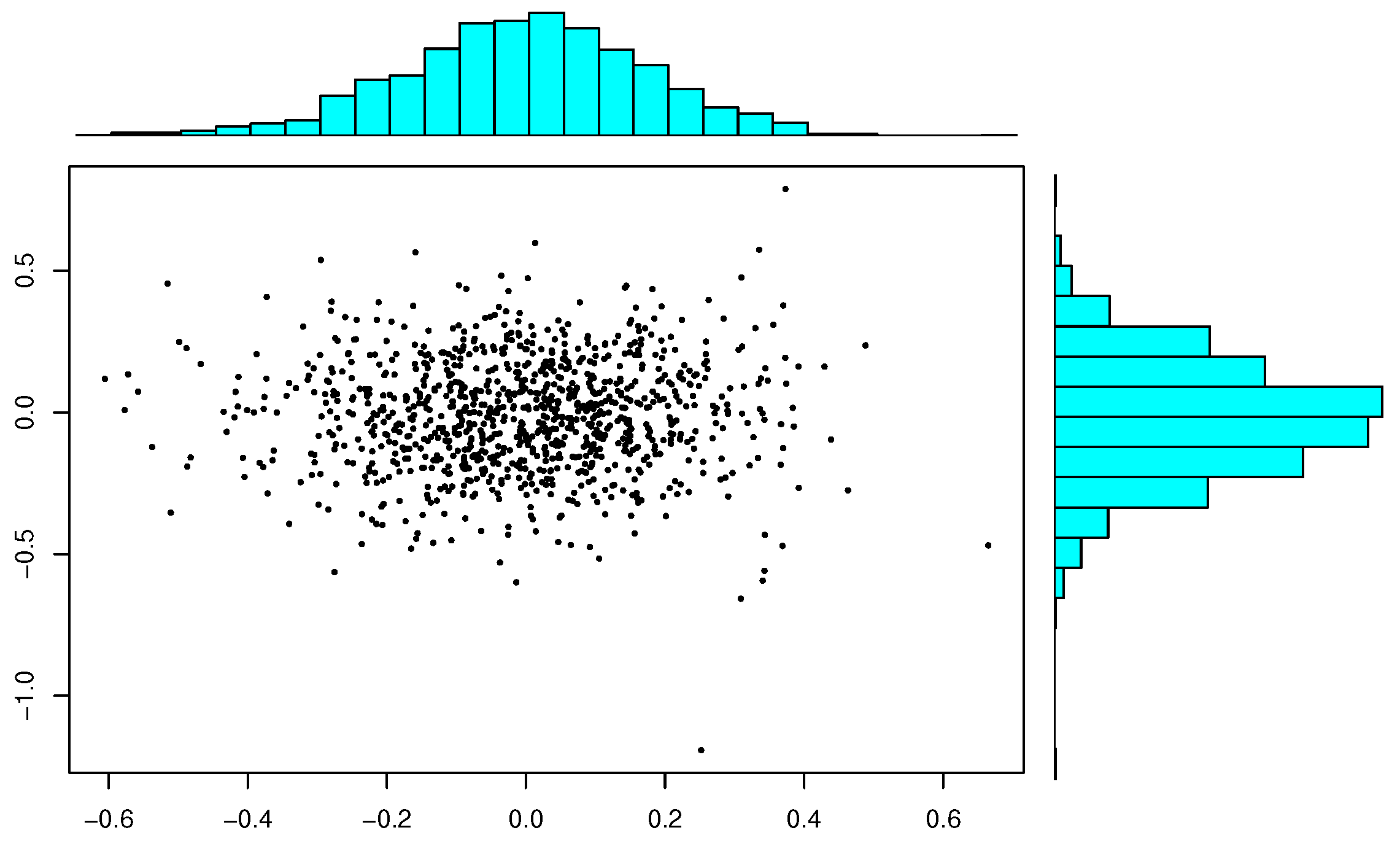
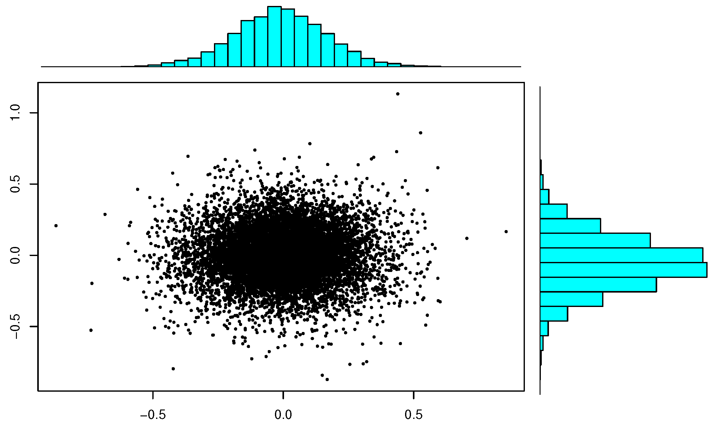
To illustrate the normality of β ^ l t s n , here, we carry out a small-scale simulation. We will generate N = 500 , 1000 , 10000   β ^ l t s n s, each obtained based on a bivariate standard normal sample { ( x i , y i ) } of size n = 50 . For each N, we provide scatter plots of N β ^ l t s n s and marginal histgrams. Inspecting Figure 1, Figure 2 and Figure 3 reveals that the plots of β ^ l t s n s more and more resemble a bivariate normal pattern when the number of β ^ l t s n increases. The marginal histograms confirm the normality.

5. Concluding Remarks

Without the population version of the LTS (see (5)), it will be difficult to apply the empirical process theory to study the asymptotics of the LTS, e.g, to verify the key result, the VC-class property of regression function class (indexed by β ) will be challenging. To avoid this challenge, some authors addressed the asymptotics of the nonlinear LTS, where without an explicit regression function (unlike the linear case), they can conveniently assume this VC-class property. Refs. [26,27] even believed that the standard empirical process theory does not apply to the asymptotics of LTS, while Refs. [22,23,24], addressed the asymptotics without any advanced tools, employing elementary tools with numerous artificial, difficult-to-verify assumptions and lengthy articles.
By partitioning the parameter space and introducing the population version for the LTS, this article establishes some fundamental and primary properties for the objective function of the LTS in both empirical and population settings. These newly obtained original results verify some key facts that were conveniently assumed (but never verified) in nonlinear regression literature for the LTS and facilitate the application of standard empirical process theory to the establishment of asymptotic normality for the sample LTS concisely and neatly. Some of the newly obtained results, such as Fisher and strong consistency, and influence function, are original and obtained as by-products.
The asymptotic normality is applied in Theorem 8 for the practical inference procedure of confidence regions of the regression parameter β 0 . There are open problems left here; one is the estimation of the variance of e, which is now unrealistically assumed to be known, and the other is the testing of the hypothesis on β 0 .

Funding

This author declares that there was no funding received for this study.

Data Availability Statement

The data will be made available by authors on request.

Acknowledgments

Insightful comments and useful suggestions from Wei Shao and Derek Young have significantly improved the manuscript and are highly appreciated. Special thanks go to Derek Young for making the technical report of Chen, Stromberg, and Zhou available.

Conflicts of Interest

This author declares that there is no conflict of interests/Competing interests.

Abbreviations

The following abbreviations are used in this manuscript:
MDPIMultidisciplinary Digital Publishing Institute
DOAJDirectory of open-access journals
TLAThree-letter acronym
LDLinear dichroism

Appendix A. Proofs

Proof of Lemma 1.
(i) Based on the definition in (9), over S β l , there is no tie among the smallest h squared residuals. The assertion (a) follows straightforwardly.
The first and the last equality in (b) is trivial, it suffices to focus on the middle one. Let k i : = k i ( η ) ( = k i ( β l ) in light of (9)). By (6), we have that
O n ( η ) = 1 n i = 1 h r k i 2 ( η ) .
Let r i : = r i ( η ) = y i w i η and γ = min { min 1 i j n { | r i 2 r j 2 | } , 1 } . Then, 1 γ > 0 (a.s.).
Based on the continuity of r k i 2 ( β ) in β , for any 1 i h and for any given ε ( 0 , 1 ) , we can fix a small δ > 0 so that | r k i 2 ( β ) r k i 2 ( η ) | < γ ε / 4 h for any β B ( η , δ ) . Now, we have for any β B ( η , δ ) , (assume below 2 i h )
r k i 2 ( β ) r k ( i 1 ) 2 ( β ) > r k i 2 ( η ) γ ε 4 h [ r k ( i 1 ) 2 ( η ) + γ ε 4 h ] = r k i 2 ( η ) r k ( i 1 ) 2 ( η ) γ ε 2 h γ γ ε 2 h > 0 ( a . s . ) ,
Thus, k i = k i ( η ) , 1 i h forms the h-integer set for any β B ( η , δ ) . Part (b) follows.
(ii) The domain of function O n ( β ) is the union of the pieces of S ¯ β l and the function of O n ( β ) over S β l is a quadratic function of β : O n ( β ) = j = 1 h r k j ( β l ) 2 ( β ) , the statement follows.
(iii) By (ii), it is clear that O n ( β ) is continuous in β over each piece of S β l . We only need to show that this holds for any β that is on the boundary of S β l .
Let η lie on the common boundary of S β s and S β t , then, O n ( β ) = 1 n i = 1 h r k i ( β s ) 2 for any β S ¯ β s [this is obviously true if β S β s , it is also true if β on the boundary of S β s since in this case the β -h-integer set is not unique, there are at least two; one of them is k 1 ( β s ) , , k h ( β s ) ] and O n ( β ) = 1 n i = 1 h r k i ( β t ) 2 for any β S ¯ β t . Let { β j } be a sequence approaching η , where β j could be on S ¯ β s or on S ¯ β t . We show that O n ( β j ) approaches to O n ( η ) . Note that O n ( η ) = 1 n i = 1 h r k i ( β s ) 2 ( η ) = 1 n i = 1 h r k i ( β t ) 2 ( η ) . Partition { β j } into { β j s } and { β j t } so that all members of the former belong to S ¯ β s where the latter are all within S ¯ β t . By continuity of the sum of h squared residuals in β , both O n ( β j s ) ) and O n ( β j t ) ) approach to O n ( η ) since both { β j s } and { β j t } approach η as min { s , t } .
(iv) Note that for any l, 1 l L , over S β l , one has a least squares problem with n reduced to h, O n ( β ) is a quadratic function and hence, is twice differentiable and strictly convex in light of the following
n β O n ( β ) = 2 i = 1 n r i 1 i w i = 2 X n D R , n 2 β 2 O n ( β ) = 2 X n D X n = 2 X * n X * n = 2 i = 1 h w k i ( β l ) w k i ( β l ) ,
where R = ( r 1 , r 2 , , r n ) , D = d i a g ( 1 i ) , and X * n = D X n . Strict convexity follows from the positive definite of the Hessian matrix: 2 n X * n X * n (an invertible matrix due to (A1), see (iii) in the proof of Theorem 1). □
Proof of Theorem 1.
(i) Over each S β l , an open set, O n ( β ) is twice differentiable and strictly convex in light of given condition, hence, it has a unique minimizer (otherwise, one can show that by openness and strictly convexity there is a third point in S β l that attains a strictly smaller objective value than the two minimizers). Since there are only finitely many S β l , the assertion follows if we can prove that the minimum does not reach a boundary point of some S β l .
Assume it is otherwise. That is, O n ( β ) reaches its global minimum at point β 1 which is a boundary point of S β l for some l. Assume that over S β l , O n ( β ) attains its local minimum value at the unique point β 2 . Then, O n ( β 1 ) O n ( β 2 ) . If equality holds, then, we have the desired result (since there are points besides β 2 in S β l which also attain the minimum value as β 2 , a contradiction). Otherwise, there is a point β 3 in the small neighborhood of β 1 so that O n ( β 3 ) O n ( β 1 ) + ( O n ( β 2 ) O n ( β 1 ) ) / 2 < O n ( β 2 ) . A contradiction appears.
(ii) It is seen from (i) that O n ( β ) is twice continuously differentiable, hence, its first derivative evaluated at the global minimum must be zero. By (i), we have the Equation (11).
(iii) This part directly follows from (ii) and the invertibility of M n . The latter follows from (A1), which implies that the p columns of matrix X n are linearly independent and also implies that any h sub-rows of X n has a full rank. □
Proof of Lemma 2.
Label G ( β ) f o r ( y w β ) 2 1 ( y w β ) 2 q ( β , α ) , the integrand in (4), for a point ( x , y ) R p . Write G ( β ) : = ( y w β ) 2 1 1 ( y w β ) 2 > q ( β , α ) .
(i) By the strictly monotonicity of F W around q ( β , α ) , we have the continuity of the q ( β , α ) . Consequently, G ( β ) is obvious continuous and so is O ( β ) in β R p .
(ii) For arbitrary points ( x , y ) and β in R p , there are three cases for the relationship between the squared residual and its quantile: (a) ( y w β ) 2 > q ( β , α ) (b) ( y w β ) 2 < q ( β , α ) , and (c) ( y w β ) 2 = q ( β , α ) . Case (c) happens with probability zero, we thus skip this case and treat (a) and (b) only. By the continuity in β , there is a small neighborhood of β : B ( β , δ ) , centered at β with radius δ such that (a) (or (b)) holds for all β B ( β , δ ) . This implies that
β 1 ( y w β ) 2 > q ( β , α ) = 0 , ( a . s . )
and
β G ( β ) = 2 ( y w β ) w 1 ( y w β ) 2 q ( β , α ) , ( a . s ) .
Hence, we have that
2 β 2 G ( β ) = 2 w w 1 ( y w β ) 2 q ( β , α ) , ( a . s ) .
Note that E ( w w ) exists. Then, by the Lebesgue-dominated convergence theorem, the desired result follows.
(iii) The strict convexity follows from the twice differentiability and the positive definite of the second order derivative of O ( β ) . □
Proof of Theorem 2.
We will treat β l t s ( F ( x , y ) , α ) , the counterpart for β l t s ( F ε ( z ) , α ) can be treated analogously.
(i) Existence follows from the positive semi-definiteness of the Hessian matrix (see proof of (ii) of Lemma 2) and the convexity of O ( β ) .
(ii) The equation follows from the differentiability and the first order derivative of O ( β ) given in the proof (ii) of Lemma 2.
(iii) The uniqueness follows from the positive definite of the Hessian matrix based on the given condition (invertibility). □
Proof of Theorem 3.
By Theorem 2, (i) and given conditions guarantee the existence and the uniqueness of β l t s ( F ( x , y ) , α ) , which is the unique solution of the system of the equations
( y w β ) w 1 ( y w β ) 2 q ( β , α ) d F ( x , y ) ( x , y ) = 0 .
Notice that y w β = w ( β β 0 ) + e . Inserting this into the above equation, we have
( w ( β β 0 ) + e ) w 1 ( w ( β β 0 ) + e ) 2 F ( w ( β β 0 ) + e ) 2 1 ( α ) d F ( x , y ) ( x , y ) = 0 .
By (ii), it is readily seen that β = β 0 is a solution of the above system of equations. Uniqueness leads to the desired result. □
Proof of Theorem 4.
Write β l t s ε ( z 0 ) for β l t s ( F ε ( z 0 ) , α ) and insert it for β into (17) and take derivative with respect to ε in both sides of (17) and let ε 0 , we obtain (in light of dominated theorem)
β l t s ε ( z 0 ) r ( β l t s ε ( z 0 ) ) v 1 r ( β l t s ε ( z 0 ) ) 2 q ε ( z , β l t s ε ( z 0 ) , α ) | ε 0 d F ( x y ) IF ( z 0 , β l t s , F ( x , y ) ) + r ( β l t s ( F ( x , y ) , α ) ) w 1 r ( β l t s ( F ( x , y ) , α ) ) 2 q ( β l t s ( F ( x , y ) , α ) , α ) d ( δ z 0 F ( x , y ) ) = 0 ,
where r ( β ) = t v β in the first term on the LHS and r ( β ) = y w β in the second term on the LHS. Call the two terms on the LHS as T 1 and T 2 , respectively, and call the integrand in T 1 as T 0 , then, it is seen that (see the proof (i) of Theorem 1)
T 0 = β l t s ε ( z 0 ) ( t v β l t s ε ( z 0 ) ) v 1 ( t v β l t s ε ( z 0 ) ) 2 q ε ( z , β l t s ε ( z 0 ) , α ) | ε 0 = w w 1 ( y w β l t s ) 2 q ( β l t s , α ) .
Focus on the T 2 , it is readily seen that
T 2 = ( y w β l t s ( F ( x , y ) , α ) ) w 1 ( y w β l t s ( F ( x , y ) , α ) ) 2 q ( β l t s ( F ( x , y ) , α ) , α ) d δ z 0 ( y w β l t s ( F ( x , y ) , α ) ) w 1 ( y w β l t s ( F ( x , y ) , α ) ) 2 q ( β l t s ( F ( x , y ) , α ) , α ) d F ( x , y ) ,
In light of (16), we have
T 2 = ( y w β l t s ( F ( x , y ) , α ) ) w 1 ( y w β l t s ( F ( x , y ) , α ) ) 2 q ( β l t s ( F ( x , y ) , α ) , α ) d δ z 0 = 0 , if ( t 0 v 0 β l t s ) 2 > q ( β l t s , α ) , ( t 0 v 0 β l t s ) v 0 , otherwise .
This, T 0 , and display (A2) lead to the desired result. □
Proof of Lemma 3.
We invoke Theorem 24 in II.5 of [32]. The first requirement of the theorem is the existence of an envelope of F . The latter is sup β Θ F r ( β ) 2 1 ( c ) , which is bounded since Θ is compact and F W 1 is continuous in β , and F W 1 ( α ) is non-decreasing in α [ 1 / 2 , c ] . To complete the proof, we only need to verify the second requirement of the theorem.
For the second requirement, that is, to bound the covering numbers, it suffices to show that the graphs of functions in F ( β , α ) have only polynomial discrimination (see Theorem 25 and Example 26 in II.5 of [32]).
The graph of a real-valued function f on a set S is defined as the subset (see p. 27 of [32])
G f = { ( s , t ) : 0 t f ( s ) or f ( s ) t 0 , s S } .
The graph of a function in F ( β , α ) contains a point ( x ( ! ) , y ( ω ) , t ) if and only if 0 t f ( x , y , β , α ) or f ( x , y , β , α ) t 0 . The latter case could be excluded since the function is always nonnegative (and equals 0 case covered by the former case). The former case happens if and only if 0 t y w β or 0 t y + w β .
Given a collection of n points ( x i , y i , t i ) ( t i 0 ), the graph of a function in F ( β , α ) picks out only points that belong to { t i 0 } { y i β w i t i 0 } { t i 0 } { y i + β w i t i 0 } . Introduce n new points ( w i , y i , z i ) : = ( ( 1 , x i ) , y i , t i ) in R p + 2 . On R p + 2 define a vector space G of functions
g a , b , c ( w , y , z ) = a w + b y + c z ,
where a R p , b R 1 , and c R 1 and G : = { g a , b , c ( w , y , z ) = a w + b y + c z , a R p , b R 1 , and c R 1 } which is a R p + 2 -dimensional vector space.
It is clear now that the graph of a function in F ( β , α ) picks out only points that belong to the sets of { g 0 } for g G (ignoring the union and intersection operations at this moment). By Lemma 18 in II.4 of [32] (p. 20), the graphs of functions in F ( β , α ) pick only polynomial numbers of subsets of { p i : = ( w i , y i , z i ) , i { 1 , , n } } ; those sets corresponding to g G with a { 0 , β , β } , b { 0 , 1 , 1 } , and c { 1 , 1 } pick up even few subsets from { p i , i { 1 , , n } } . This in conjunction with Lemma 15 in II.4 of [32] (p. 18), yields that the graphs of functions in F ( β , α ) have only polynomial discrimination. By Theorem 24 in II.5 of [32], we have completed the proof. □
Proof of Theorem 6.
To apply Lemma 4, we need to verify the five conditions; among them, only (iii) and (v) need to be addressed, and all others are satisfied trivially. For (iii), it holds automatically since our τ n = β ^ l t s n is defined to be the minimizer of F n ( t ) over t T ( = Θ ) .
So, the only condition that needs to be verified is (v), the stochastic equicontinuity of { E n r ( · , t ) } at t 0 . For that, we will appeal to the Equicontinuity Lemma (VII.4 of [32], p. 150). To apply the Lemma, we will verify the condition for the random covering numbers satisfy the uniformity condition. To that end, we look at the class of functions
R ( β , α ) = r ( · , · , α , β ) = β β V / 2 β β β : β Θ , α [ 1 / 2 , c ] .
Obviously, λ m a x r 0 / 2 is an envelope for the class R in L 2 ( P ) , where r 0 is the radius of the ball Θ = B ( β l t s , r 0 ) . We now show that the covering numbers of R is uniformly bounded, which amply suffices for the Equicontinuity Lemma. For this, we will invoke Lemmas II.25 and II.36 of [32]. To apply Lemma II.25, we need to show that the graphs of functions in R have only polynomial discrimination. The graph of r ( x , y , α , β ) contains a point ( x , y , t ) , t 0 if and only if β β V / 2 β β β t for all β Θ and α [ 1 / 2 , c ] .
Equivalently, the graph of r ( x , y , α , β ) contains a point ( x , y , t ) , t 0 if and only if λ m i n / 2 β t . For a collection of n points ( x i , y i , t i ) with t i 0 , the graph picks out those points satisfying λ m i n / 2 β t i 0 . Construct from ( x i , y i , t i ) , a point z i = t i in R . On R , define a vector space G of functions
g a , b ( x ) = a x + b , a , b R .
By Lemma 18 of [32], the sets { g 0 } , for g G , pick out only a polynomial number of subsets from { z i } ; those sets corresponding to functions in G with a = 1 and b = λ m i n / 2 β pick out even fewer subsets from { z i } . Thus, the graphs of functions in R have only polynomial discrimination. □
Proof of Theorem 8.
In order to invoke Theorem 6, we only need to check the uniqueness of β ^ l t s n and β l t s . The former is guaranteed by the (iii) of Theorem 1 since (A1) holds true a.s. This is because any p columns of the X n or any of its h rows could be regarded as a sample from an continuous random vector with dimension n or h. The probability that these p points lie in a ( p 1 ) dimensional non-degenerated hyperplane (the normal vector is non-zero) is zero.
The latter is guaranteed by (iii) of Theorem 2 since W = ( y w β ) 2 is the square of a normal distribution with mean β 1 and hence, has a positive density and (18) becomes 2 ( Φ ( c / σ ) 1 / 2 ) I p × p , hence, is invertible, where c is defined in Theorem 8. By Theorems 3 and 7, we can assume, w.l.o.g., that β l t s = β 0 = 0 . Utilizing the independence between e and x and Theorem 6, a straightforward calculation leads to the results. □

References

  1. Rousseeuw, P.J.; Leroy, A. Robust Regression and Outlier Detection; Wiley: New York, NY, USA, 1987. [Google Scholar]
  2. Huber, P.J. Robust estimation of a location parameter. Ann. Math. Stat. 1964, 35, 73–101. [Google Scholar] [CrossRef]
  3. Rousseeuw, P.J. Least median of squares regression. J. Am. Stat. Assoc. 1984, 79, 871–880. [Google Scholar] [CrossRef]
  4. Rousseeuw, P.J.; Yohai, V.J. Robust regression by means of S-estimators. In Robust and Nonlinear Time Series Analysis; Lecture Notes in Statistics; Springer: New York, NY, USA, 1984; Volume 26, pp. 256–272. [Google Scholar]
  5. Yohai, V.J. High breakdown-point and high efficiency estimates for regression. Ann. Stat. 1987, 15, 642–656. [Google Scholar] [CrossRef]
  6. Yohai, V.J.; Zamar, R.H. High breakdown estimates of regression by means of the minimization of an efficient scale. J. Am. Stat. Assoc. 1988, 83, 406–413. [Google Scholar] [CrossRef]
  7. Rousseeuw, P.J.; Hubert, M. Regression depth (with discussion). J. Am. Stat. Assoc. 1999, 94, 388–433. [Google Scholar] [CrossRef]
  8. Zuo, Y. On general notions of depth for regression. Stat. Sci. 2021, 36, 142–157. [Google Scholar] [CrossRef]
  9. Zuo, Y. Robustness of the deepest projection regression depth functional. Stat. Pap. 2021, 62, 1167–1193. [Google Scholar] [CrossRef]
  10. Rousseeuw, P.J.; Van Driessen, K. Computing LTS Regression for Large Data Sets. Data Min. Knowl. Discov. 2006, 12, 29–45. [Google Scholar] [CrossRef]
  11. Stromberg, A.J. Computation of High Breakdown Nonlinear Regression Parameters. J. Am. Stat. Assoc. 1993, 88, 237–244. [Google Scholar] [CrossRef]
  12. Hawkins, D.M. The feasible solution algorithm for least trimmed squares regression. Comput. Stat. Data Anal. 1994, 17, 185–196. [Google Scholar] [CrossRef]
  13. Hössjer, O. Exact computation of the least trimmed squares estimate in simple linear regression. Comput. Stat. Data Anal. 1995, 19, 265–282. [Google Scholar] [CrossRef]
  14. Rousseeuw, P.J.; Van Driessen, K. A fast algorithm for the minimum covariance determinant estimator. Technometrics 1999, 41, 212–223. [Google Scholar] [CrossRef]
  15. Hawkins, D.M.; Olive, D.J. Improved feasible solution algorithms for high breakdown estimation. Comput. Stat. Data Anal. 1999, 30, 1–11. [Google Scholar] [CrossRef]
  16. Agullö, J. New algorithms for computing the least trimmed squares regression estimator. Comput. Stat. Data Anal. 2001, 36, 425–439. [Google Scholar] [CrossRef]
  17. Hofmann, M.; Gatu, C.; Kontoghiorghes, E.J. An Exact Least Trimmed Squares Algorithm for a Range of Coverage Values. J. Comput. Andgr. Stat. 2010, 19, 191–204. [Google Scholar] [CrossRef]
  18. Klouda, K. An Exact Polynomial Time Algorithm for Computing the Least Trimmed Squares Estimate. Comput. Stat. Data Anal. 2015, 84, 27–40. [Google Scholar] [CrossRef]
  19. Alfons, A.; Croux, C.; Gelper, S. Sparse least trimmed squares regression for analyzing high-dimensional large data sets. Ann. Appl. Stat. 2013, 7, 226–248. [Google Scholar] [CrossRef]
  20. Kurnaz, F.S.; Hoffmann, I.; Filzmoser, P. Robust and sparse estimation methods for high-dimensional linear and logistic regression. Chemom. Intell. Lab. Syst. 2018, 172, 211–222. [Google Scholar] [CrossRef]
  21. Mašíček, L. Optimality of the Least Weighted Squares Estimator. Kybernetika 2004, 40, 715–734. [Google Scholar]
  22. Všek, J.Á. The least trimmed squares. Part I: Consistency. Kybernetika 2006, 42, 1–36. [Google Scholar]
  23. Všek, J.Á. The least trimmed squares. Part II: n -consistency. Kybernetika 2006, 42, 181–202. [Google Scholar]
  24. Všek, J.Á. The least trimmed squares. Part III: Asymptotic normality. Kybernetika 2006, 42, 203–224. [Google Scholar]
  25. Chen, Y.; Stromberg, A.; Zhou, M. The Least Trimmed Squares Estimate in Nonlinear Regression; Technical Report, 1997/365; Department of Statistics, University of Kentucky: Lexington, KY, USA, 1997. [Google Scholar]
  26. Čížek, P. Asymptotics of Least Trimmed Squares Regression; CentER Discussion Paper 2004-72; Tilburg University: Tilburg, The Netherlands, 2004. [Google Scholar]
  27. Čížek, P. Least Trimmed Squares in nonlinear regression under dependence. J. Stat. Plan. Inference 2005, 136, 3967–3988. [Google Scholar] [CrossRef]
  28. Zuo, Y.; Zuo, H. Least sum of squares of trimmed residuals regression. Electron. J. Stat. 2023, 17, 2447–2484. [Google Scholar] [CrossRef]
  29. Hampel, F.R.; Ronchetti, E.M.; Rousseeuw, P.J.; Stahel, W.A. Robust Statistics: The Approach Based on Influence Functions; John Wiley & Sons: New York, NY, USA, 1986. [Google Scholar]
  30. Tableman, M. The influence functions for the least trimmed squares and the least trimmed absolute deviations estimators. Stat. Probab. Lett. 1994, 19, 329–337. [Google Scholar] [CrossRef]
  31. Öllerer, V.; Croux, C.; Alfons, A. The influence function of penalized regression estimators. Statistics 2015, 49, 741–765. [Google Scholar] [CrossRef]
  32. Pollard, D. Convergence of Stochastic Processes; Springer: Berlin, Germany, 1984. [Google Scholar]
  33. Bednarski, T.; Clarke, B.R. Trimmed likelihood estimation of location and scale of the normal distribution. Aust. J. Stat. 1993, 35, 141–153. [Google Scholar] [CrossRef]
  34. Butler, R.W. Nonparametric interval point prediction using data trimmed by a Grubbs type outlier rule. Ann. Stat. 1982, 10, 197–204. [Google Scholar] [CrossRef]
  35. Hössjer, O. Rank-Based Estimates in the Linear Model with High Breakdown Point. J. Am. Stat. Assoc. 1994, 89, 149–158. [Google Scholar] [CrossRef]
  36. Zuo, Y. A new approach for the computation of halfspace depth in high dimensions. Commun. Stat. Simul. Comput. 2018, 48, 900–921. [Google Scholar] [CrossRef]
  37. Zuo, Y. Projection-based depth functions and associated medians. Ann. Stat. 2003, 31, 1460–1490. [Google Scholar] [CrossRef]
  38. Shao, W.; Zuo, Y.; Luo, J. Employing the MCMC Technique to Compute the Projection Depth in High Dimensions. J. Comput. Appl. Math. 2022, 411, 114278. [Google Scholar] [CrossRef]
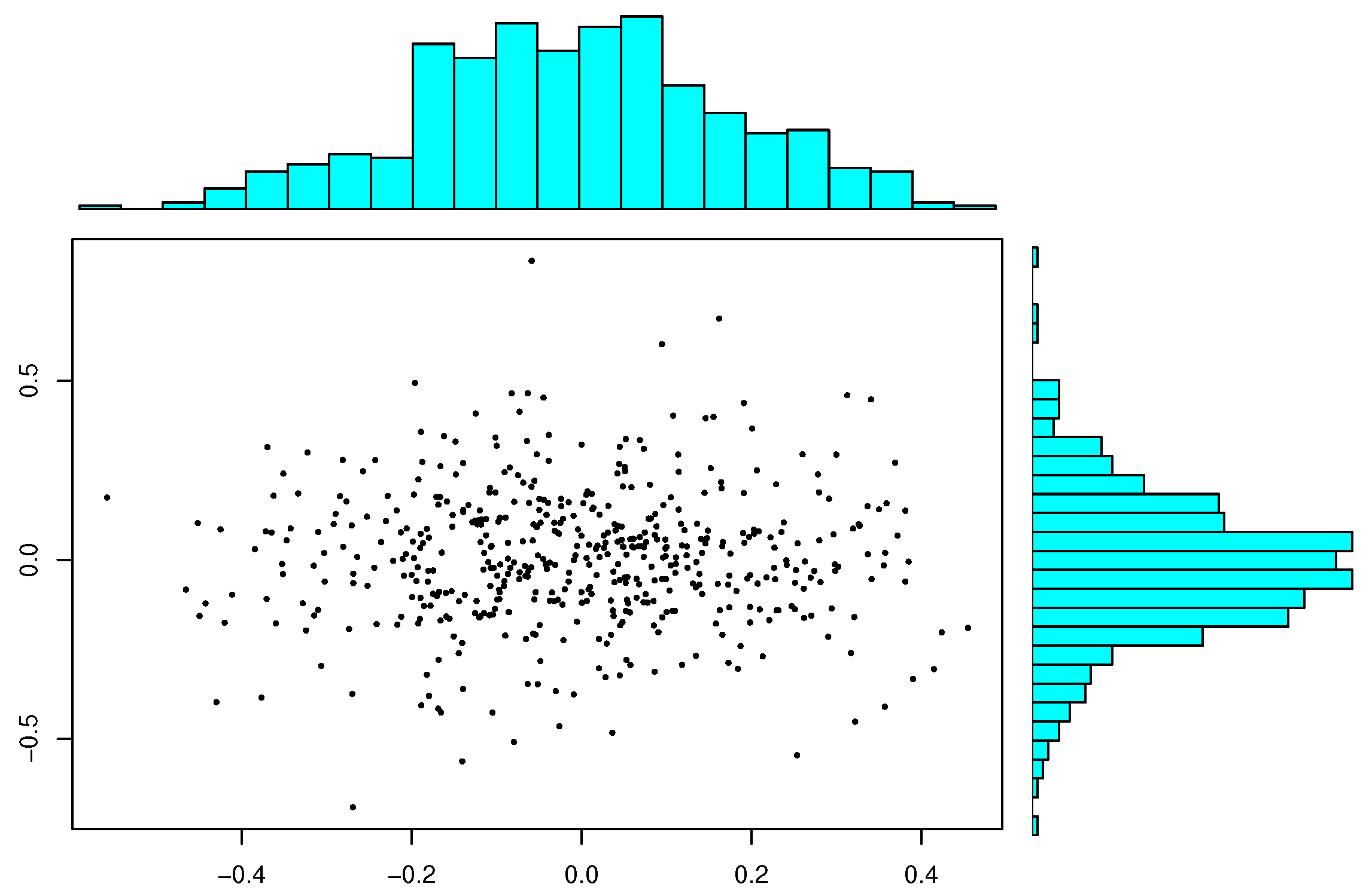
Figure 1. Marginal histograms and scatter plot of 500 β ^ l t s n with sample size n = 50 .
Mathematics 12 03586 g001
Figure 2. Marginal histograms and scatter plot of 1000 β ^ l t s n with sample size n = 50 .
Mathematics 12 03586 g002
Figure 3. Marginal histograms and scatter plot of 10000 β ^ l t s n with sample size n = 50 .
Mathematics 12 03586 g003
Disclaimer/Publisher’s Note: The statements, opinions and data contained in all publications are solely those of the individual author(s) and contributor(s) and not of MDPI and/or the editor(s). MDPI and/or the editor(s) disclaim responsibility for any injury to people or property resulting from any ideas, methods, instructions or products referred to in the content.