A Study of Szász–Durremeyer-Type Operators Involving Adjoint Bernoulli Polynomials

Abstract

This research work introduces a connection of adjoint Bernoulli’s polynomials and a gamma function as a sequence of linear positive operators. Further, the convergence properties of these sequences of operators are investigated in various functional spaces with the aid of the Korovkin theorem, Voronovskaja-type theorem, first order of modulus of continuity, second order of modulus of continuity, Peetre’s K-functional, Lipschitz condition, etc. In the last section, we extend our research to a bivariate case of these sequences of operators, and their uniform rate of approximation and order of approximation are investigated in different functional spaces. Moreover, we construct a numerical example to demonstrate the applicability of our results.

1. Introduction and Preliminaries

It is well known that S. Bernstein (1913 [1]) proposed a sequence of the following polynomials to prove the Weierstrass theorem [2] on the possibility of a uniform approximation of continuous functions on a segment by sequences of polynomials:

$$\begin{array}{c}\hfill B_r(\hslash ;\mu )=\sum _{\nu =0}^r{p}_{r,\nu }\left(\mu \right)\hslash \left({\displaystyle \frac{\nu }{r}}\right),r\in \mathbb{N},\end{array}$$

(1)

where $p_{r,\nu }\left(\mu \right)=\left({\displaystyle \genfrac{}{}{0pt}{}{r}{\nu }}\right){\mu }^{\nu }{(1-\mu )}^{\nu -r}$. He found that $B_r(\hslash ;.)$ converges uniformly on $[0,1]$ as $r\to +\infty$ to the function ℏ. In the past decade, many mathematicians have constructed various modifications of the operators defined by (1) to achieve better flexibility in approximation properties over bounded and unbounded intervals in various functional spaces, e.g., Aslan et al. [3] studied the rate of approximation of blending-type modified univariate and bivariate $\lambda$-Schurer–Kantorovich operators, Leinartas et al. [4] introduced the discrete analogue of the Newton–Leibniz formula into the problem of summation over simple lattice points, Mohiuddine et al. [5] constructed a family of Bernstein–Kantorovich operators to approximate in a Lebesgue measurable class, Rao et al. [6,7] discussed blending-type approximations by a Kantorovich variant of an $\alpha$-Baskakov operator and two-dimensional Chlodowsky–Szász operators via Sheffer polynomials, etc.

In view of polynomials classes, which is an active field of research and a special function field of research, we recall a class of polynomials by Appell [8] termed Appell polynomials, ${\left\{p_{\nu }\left(\mu \right)\right\}}_{\nu =0}^{\infty }$, associated with the generating function as follows:

$$A\left(t\right)e^{\mu t}=\sum _{\nu =0}^{\infty }{p}_{\nu }\left(\mu \right){\displaystyle \frac{t^{\nu }}{\nu !}},$$

(2)

where $A\left(t\right)={\displaystyle \sum _{\nu =0}^{\infty }}{a}_{\nu }{\displaystyle \frac{t^{\nu }}{\nu !}},A\left(0\right)=0,$ which is an analytic function at $t=0$ such that $a_{\nu }=p_{\nu }\left(0\right).$ Recently, Natalini et al. [9] gave Appell Bernoulli polynomials, choosing $A\left(t\right)={\displaystyle \frac{t}{e^t-1}}$ in (2). Adjoint Bernoulli polynomials choosing $A\left(t\right)$ as ${\displaystyle \frac{1}{A\left(t\right)}}$ in the generating function are denoted as ${\left\{{\beta }_{\nu }\left(\mu \right)\right\}}_{\nu =0}^{\infty }$ and defined by the exponential-type generating function:

$${\displaystyle \frac{e^t-1}{t}}{e}^{\mu t}=\sum _{\nu =0}^{\infty }{\displaystyle \frac{{\beta }_{\nu }\left(\mu \right)t^{\nu }}{\nu !}}.$$

(3)

The adjoint Bernoulli polynomials defined in (3) are positive on $[0,\infty )$. Such types of generating functions are the central attraction for readers who are fascinated by the field of operator theory from other perspectives, e.g., [10,11,12,13,14].

Motivated by the above literature, we construct a new connection of adjoint Bernoulli polynomials coupling a gamma function as a new sequence of positive linear operators as follows:

$${\tilde{G}}_{r,\lambda }(\hslash ;\mu )=\sum _{\nu =0}^{\infty }{g}_{\nu }\left(a_r\mu \right){\int }_0^{\infty }{b}_{c_r,\nu }\left(\theta \right)\hslash \left(\theta \right)d\theta ,$$

(4)

where ${\left\{a_r\right\}}_1^{\infty }$, ${\left\{c_r\right\}}_1^{\infty }$ are increasing sequences of real numbers such that $\underset{r\to \infty }{lim}{a}_r=\underset{r\to \infty }{lim}{c}_r=\infty$, ${\displaystyle \frac{a_r}{c_r}}=1+{\displaystyle \frac{1}{c_r}}$, $\hslash \in L_{\beta }[0,\infty )$ (a space of Lebesgue measurable and bounded functions) and $g_{\nu }\left(a_r\mu \right)={\displaystyle \frac{e^{-a_r\mu }}{e-1}}{\displaystyle \frac{{\beta }_{\nu }\left(a_r\mu \right)}{\nu !}}$, $b_{c_r,\nu }^{\lambda }\left(\theta \right)={\displaystyle \frac{c_r^{\nu +\lambda +1}}{\mathsf{\Gamma }\left(\nu +\lambda \right)}}{\theta }^{\nu +\lambda }{e}^{-c_r\theta }$. Here, we discuss some preliminaries in order to discuss the approximation properties of ${\tilde{G}}_{r,\lambda }(.;.)$ in (4) as follows:

Lemma 1 

([15]). For $\mu \in [0,\infty )$ and the generating function given by (3), we have

$$\begin{array}{cc}\hfill \sum _{\nu =0}^{\infty }{\displaystyle \frac{{\beta }_{\nu }\left(r\mu \right)}{\nu !}}& =e^{r\mu }(e-1),\hfill \\ \hfill \sum _{\nu =0}^{\infty }\nu {\displaystyle \frac{{\beta }_{\nu }\left(r\mu \right)}{\nu !}}& =r\mu e^{r\mu }(e-1)+e^{r\mu },\hfill \\ \hfill \sum _{\nu =0}^{\infty }{\nu }^2{\displaystyle \frac{{\beta }_{\nu }\left(r\mu \right)}{\nu !}}& =r^2{\mu }^2{e}^{r\mu }(e-1)+r\mu e^{r\mu }(e+1)+e^{r\mu }(e-1),\hfill \\ \hfill \sum _{\nu =0}^{\infty }{\nu }^3{\displaystyle \frac{{\beta }_{\nu }\left(r\mu \right)}{\nu !}}& =r^3{\mu }^3{e}^{r\mu }(e-1)+r^2{\mu }^2{e}^{r\mu }3e+r\mu e^{r\mu }(4e-1)+e^r\mu (e+1),\hfill \\ \hfill \sum _{\nu =0}^{\infty }{\nu }^4{\displaystyle \frac{{\beta }_{\nu }\left(r\nu \right)}{\nu !}}& =r^4{\mu }^4{e}^{r\mu }(e-1)+r^3{\mu }^3{e}^{r\mu }(6e-2)+r^2{\mu }^2{e}^{r\mu }(13e-1)\hfill \\ \hfill & +r\mu e^{r\mu }(11e+1)+e^{r\mu }(4e-1).\hfill \end{array}$$

Lemma 2. 

For $\mu \in [0,\infty )$ and the generating function given by (3), we have

$$\begin{array}{cc}\hfill \sum _{\nu =0}^{\infty }{\displaystyle \frac{{\beta }_{\nu }\left(a_r\mu \right)}{\nu !}}& =e^{a_r\mu }(e-1),\hfill \\ \hfill \sum _{\nu =0}^{\infty }\nu {\displaystyle \frac{{\beta }_{\nu }\left(a_r\mu \right)}{\nu !}}& =a_r\mu e^{a_r\mu }(e-1)+e^{a_r\mu },\hfill \\ \hfill \sum _{\nu =0}^{\infty }{\nu }^2{\displaystyle \frac{{\beta }_{\nu }\left(a_r\mu \right)}{\nu !}}& =a_r^2{\mu }^2{e}^{a_r\mu }(e-1)+a_r\mu e^{a_r\mu }(e+1)+e^{a_r\mu }(e-1),\hfill \\ \hfill \sum _{\nu =0}^{\infty }{\nu }^3{\displaystyle \frac{{\beta }_{\nu }\left(a_r\mu \right)}{\nu !}}& =a_r^3{\mu }^3{e}^{a_r\mu }(e-1)+a_r^2{\mu }^2{e}^{a_r\mu }3e+a_r\mu e^{a_r\mu }(4e-1)+e^{a_r\mu }(e+1),\hfill \\ \hfill \sum _{\nu =0}^{\infty }{\nu }^4{\displaystyle \frac{{\beta }_{\nu }\left(a_r\nu \right)}{\nu !}}& =a_r^4{\mu }^4{e}^{a_r\mu }(e-1)+a_r^3{\mu }^3{e}^{a_r\mu }(6e-2)+a_r^2{\mu }^2{e}^{a_r\mu }(13e-1)\hfill \\ \hfill & +a_r\mu e^{a_r\mu }(11e+1)+e^{a_r\mu }(4e-1).\hfill \end{array}$$

Proof. 

In the direction of Lemma (1) and replacing $r=a_r$ defined in (4), we can simply arrive at the desired result. □

Lemma 3. 

Let ${\hslash }_j\left(\theta \right)={\theta }^j$, $j\in \{0,1,2,3,4\}$. Then, the following equalities hold:

$$\begin{array}{cc}\hfill {\tilde{G}}_{r,\lambda }(1;\mu )& =1,\hfill \\ \hfill {\tilde{G}}_{r,\lambda }({\hslash }_1,\mu )& ={\displaystyle \frac{a_r}{c_r}}\mu +{\displaystyle \frac{1}{c_r}}\left({\displaystyle \frac{\lambda (e-1)+1}{e-1}}\right),\hfill \\ \hfill {\tilde{G}}_{r,\lambda }({\hslash }_2,\mu )& ={\left({\displaystyle \frac{a_r}{c_r}}\right)}^2{\mu }^2+{\displaystyle \frac{a_r}{c_r^2}}(2e(\lambda +1)-2\lambda )\mu +{\displaystyle \frac{1}{c_r^2}}\left(1+{\displaystyle \frac{2\lambda +1}{e-1}}+{\lambda }^2+\lambda \right),\hfill \\ \hfill {\tilde{G}}_{r,\lambda }({\hslash }_3,\mu )& ={\left({\displaystyle \frac{a_r}{c_r}}\right)}^3{\mu }^3+{\displaystyle \frac{a_r^2}{c_r^3}}\left[3e(\lambda +2)-3(\lambda +1)\right]{\mu }^2+{\displaystyle \frac{a_r}{c_r^3}}[3{\lambda }^2(e-1)+3\lambda (3e-1)\hfill \\ \hfill & +3(3e-1)]\mu +{\displaystyle \frac{1}{c_r^3}}\left[{\lambda }^3+6{\lambda }^2+8\lambda +3+{\displaystyle \frac{e+1}{e-1}}\right],\hfill \\ \hfill {\tilde{G}}_{r,\lambda }({\hslash }_4,\mu )& ={\left({\displaystyle \frac{a_r}{c_r}}\right)}^4{\mu }^4+o\left({\displaystyle \frac{1}{c_r}}\right).\hfill \end{array}$$

Proof. 

To prove Lemma (3), we call operators ${\tilde{G}}_{r,\lambda }(.,.)$ in (4) as follows:

$$\begin{array}{c}\hfill {\tilde{G}}_{r,\lambda }({\hslash }_j;\mu )={\displaystyle \frac{e^{-a_r\mu }}{e-1}}\sum _{\nu =0}^{\infty }{\displaystyle \frac{{\beta }_{\nu }\left(a_r\mu \right)}{\nu !}}{\int }_0^{\infty }{b}_{c_r,\nu }\left(\theta \right){\theta }^{j}d\theta .\end{array}$$

(5)

For $j=0$, ${\int }_0^{\infty }{b}_{c_r,\nu }\left(\theta \right)d\theta =1$, which implies that

$$\begin{array}{c}\hfill {\tilde{G}}_{r,\lambda }({\hslash }_0;\mu )={\displaystyle \frac{e^{-a_r\mu }}{e-1}}\sum _{\nu =0}^{\infty }{\displaystyle \frac{{\beta }_{\nu }\left(a_r\mu \right)}{\nu !}}=1.\end{array}$$

For $j=1$,

$$\begin{array}{cc}\hfill {\int }_0^{\infty }{b}_{c_r,\nu }\left(\theta \right)\theta d\theta & ={\displaystyle \frac{c_r^{\nu +\lambda +1}}{\mathsf{\Gamma }\left(\nu +\lambda \right)}}{\int }_0^{\infty }{\theta }^{\nu +\lambda +1}{e}^{-c_r\theta }d\theta \hfill \\ \hfill \hspace{1em}& ={\displaystyle \frac{c_r^{\nu +\lambda +1}}{\mathsf{\Gamma }\left(\nu +\lambda \right)}}{\displaystyle \frac{\mathsf{\Gamma }\left(\nu +\lambda +1\right)}{c_r^{\nu +\lambda +2}}}={\displaystyle \frac{\nu +\lambda }{c_r}}.\hfill \end{array}$$

(6)

Clubbing Equations (5) and (6), we obtain

$$\begin{array}{c}\hfill {\tilde{G}}_{r,\lambda }({\hslash }_1;\mu )={\displaystyle \frac{1}{c_r}}\left[{\displaystyle \frac{e^{-a_r\mu }}{e-1}}\sum _{\nu =0}^{\infty }{\displaystyle \frac{\nu {\beta }_{\nu }\left(a_r\mu \right)}{\nu !}}\right]+{\displaystyle \frac{\lambda }{c_r}}.\end{array}$$

In view of Lemma (2), we obtain

$$\begin{array}{cc}\hfill {\tilde{G}}_{r,\lambda }({\hslash }_1,\mu )& ={\displaystyle \frac{a_r}{c_r}}\mu +{\displaystyle \frac{1}{c_r}}\left({\displaystyle \frac{\lambda (e-1)+1}{e-1}}\right).\end{array}$$

For $j=2$,

$$\begin{array}{cc}\hfill {\int }_0^{\infty }{b}_{c_r,\nu }\left(\theta \right){\theta }^{2}d\theta & ={\displaystyle \frac{c_r^{\nu +\lambda +1}}{\mathsf{\Gamma }\left(\nu +\lambda \right)}}{\int }_0^{\infty }{\theta }^{\nu +\lambda +2}{e}^{-c_r\theta }d\theta \hfill \\ \hfill \hspace{1em}& ={\displaystyle \frac{c_r^{\nu +\lambda +1}}{\mathsf{\Gamma }\left(\nu +\lambda \right)}}{\displaystyle \frac{\mathsf{\Gamma }\left(\nu +\lambda +2\right)}{c_r^{\nu +\lambda +3}}}={\displaystyle \frac{(\nu +\lambda +1)(\nu +\lambda )}{c_r^2}}.\hfill \end{array}$$

(7)

Clubbing Equations (5) and (7), we obtain

$$\begin{array}{c}\hfill {\tilde{G}}_{a_r,\lambda }({\hslash }_2;\mu )=\left[{\displaystyle \frac{e^{-a_r\mu }}{e-1}}\sum _{\nu =0}^{\infty }{\displaystyle \frac{{\beta }_{\nu }\left(a_r\mu \right)}{\nu !}}\right]{\displaystyle \frac{(\nu +\lambda +1)(\nu +\lambda )}{c_r^2}}.\end{array}$$

In view of Lemma (2), we obtain

$$\begin{array}{cc}\hfill {\tilde{G}}_{r,\lambda }({\hslash }_2,\mu )& ={\left({\displaystyle \frac{a_r}{c_r}}\right)}^2{\mu }^2+{\displaystyle \frac{a_r}{c_r^2}}(2e(\lambda +1)-2\lambda )\mu +{\displaystyle \frac{1}{c_r^2}}\left(1+{\displaystyle \frac{2\lambda +1}{e-1}}+{\lambda }^2+\lambda \right).\end{array}$$

Similarly, the rest of this Lemma can be proved very easily. □

Lemma 4. 

For the sequence of operators presented by (4) and ${\hslash }_j^{\mu }\left(\theta \right)={(\theta -\mu )}^j$, one has the following equalities:

$$\begin{array}{ccc}\hfill {\tilde{G}}_{r,\lambda }({\hslash }_o^{\mu };\mu )& =& 1,\hfill \\ \hfill {\tilde{G}}_{r,\lambda }({\hslash }_1^{\mu };\mu )& =& {\displaystyle \frac{1}{c_r}}\left(\mu +{\displaystyle \frac{\lambda (e-1)+1}{e-1}}\right),\hfill \\ \hfill {\tilde{G}}_{r,\lambda }({\hslash }_2^{\mu };\mu )& =& {\displaystyle \frac{{\mu }^2}{c_r^2}}+{\displaystyle \frac{a_r}{c_r^2}}\left(2e(\lambda +1)-2\lambda -2\left({\displaystyle \frac{\lambda (e-1)+1}{e-1}}\right)\right)\mu \hfill \\ \hspace{1em}& +& {\displaystyle \frac{1}{c_r^2}}\left(1+{\displaystyle \frac{2\lambda +1}{e-1}}+{\lambda }^2+\lambda \right),\hfill \\ \hfill {\tilde{G}}_{r,\lambda }({\hslash }_4^{\mu };\mu )& =& o\left({\displaystyle \frac{1}{c_r^2}}\right){\mu }^2.\hfill \end{array}$$

Proof. 

In the light of operators (4) and the linearity property, we obtain

$$\begin{array}{ccc}\hfill {\tilde{G}}_{r,\lambda }({\hslash }_o^{\mu };\mu )& =& {\tilde{G}}_{r,\lambda }(1;\mu )=1,\hfill \\ \hfill {\tilde{G}}_{r,\lambda }({\hslash }_1^{\mu };\mu )& =& {\tilde{G}}_{r,\lambda }(\theta -\mu ;\mu )={\tilde{G}}_{r,\lambda }({\hslash }_1;\mu )-\mu {\tilde{G}}_{r,\lambda }(1;\mu ),\hfill \\ \hfill {\tilde{G}}_{r,\lambda }({\hslash }_2^{\mu };\mu )& =& {\tilde{G}}_{r,\lambda }({(\theta -\mu )}^2;\mu )={\tilde{G}}_{r,\lambda }({\hslash }_2;\mu )-2\mu {\tilde{G}}_{r,\lambda }({\hslash }_1;\mu )+{\mu }^2{\tilde{G}}_{r,\lambda }(1;\mu ).\hfill \end{array}$$

In this direction, we can arrive at the desired result. □

Remark 1. 

The sequences of operators given in (4) are linear, i.e., for all $k_1,k_2\in \mathbb{R}$ and ${\theta }_1,$${\theta }_2\in [0,\infty )$, we have

$$\begin{array}{c}\hfill {\tilde{G}}_{r,\lambda }(k_1{\theta }_1+k_2{\theta }_2;\mu )=k_1{\tilde{G}}_{r,\lambda }({\theta }_1;\mu )+k_2{\tilde{G}}_{r,\lambda }({\theta }_2;\mu ).\end{array}$$

Remark 2. 

The sequences of operators given in (4) are positive, i.e., ${\tilde{G}}_{r,\lambda }(\hslash ;\mu )\ge 0$ for $\hslash \ge 0$.

To present the approximation properties of the sequences of operators given by (4), we draft the present manuscript with some subsequent sections on the following: the uniform rate of convergence, direct approximation properties, weighted approximation properties and bivariate extension of the operators given by (4) with their rate of convergence and order of approximations in various functional spaces to achieve better approximation behaviour in terms of these sequences of operators.

2. Approximation Properties: Uniform Rate of Convergence and Order of Approximation

Definition 1 

([16]). Let $\hslash \in C_B[0,\infty )$. Then, the modulus of continuity is defined as

$$\begin{array}{c}\hfill \omega (\hslash ;\tilde{\delta })=\underset{|{\mu }_1-{\mu }_2|\le \tilde{\delta }}{sup}|\hslash \left({\mu }_1\right)-\hslash \left({\mu }_2\right)|,{\mu }_1,{\mu }_2\in [0,\infty ),\end{array}$$

(8)

and

$$\begin{array}{c}\hfill |\hslash \left({\mu }_1\right)-\hslash \left({\mu }_2\right)|\le \left(1+{\displaystyle \frac{|{\mu }_1-{\mu }_2|}{\tilde{\delta }}}\right)\omega (\hslash ;\tilde{\delta }).\end{array}$$

(9)

Theorem 1. 

Let ${\tilde{G}}_{r,\lambda }(.;.)$ be given in (4). Then, ${\tilde{G}}_{r,\lambda }(\hslash ;.)$ converges uniformly to ℏ on a bounded subinterval of $[0,\infty )$.

Proof. 

On account of the classical Korovkin theorem [17], it is sufficient to show that

$$\begin{array}{c}\hfill {\tilde{G}}_{r,\lambda }({\theta }^j;\mu )={\mu }^j, j\in \{0,1,2\},\end{array}$$

uniformly on each closed and bounded subset of $[0,\infty ).$ Using Lemma (3), we arrive at the desired result immediately. □

The next result is the study of the order of approximation of (4) in terms of the modulus of continuity in Equation (8):

Theorem 2. 

For $\hslash \in C_B[0,\infty )$ (space of bounded and continuous functions) and the sequence of operators ${\tilde{G}}_{r,\lambda }(.;.)$ in Equation (4), we have

$$\begin{array}{c}\hfill |{\tilde{G}}_{r,\lambda }(\hslash ;\mu )-\hslash \left(\mu \right)|\le 2\omega (\hslash ;\tilde{\delta }),\end{array}$$

where $\tilde{\delta }=\sqrt{{\tilde{G}}_{r,\lambda }({\hslash }_2^{\mu };\mu )}$.

Proof. 

With the definition of Equation (4), we have

$$\begin{array}{ccc}\hfill |{\tilde{G}}_{r,\lambda }(\hslash ;\mu )-\hslash \left(\mu \right)|& =& \left|{\displaystyle \frac{e^{-a_r\mu }}{e-1}}\sum _{\nu =0}^{\infty }{\displaystyle \frac{{\beta }_{\nu }\left(a_r\mu \right)}{\nu !}}{\int }_0^{\infty }{b}_{c_r,\nu }\left(\theta \right)\{\hslash \left(\theta \right)-\hslash \left(\mu \right)\}d\theta \right|,\hfill \\ \hspace{1em}& \le & {\displaystyle \frac{e^{-a_r\mu }}{e-1}}\sum _{\nu =0}^{\infty }{\displaystyle \frac{{\beta }_{\nu }\left(a_r\mu \right)}{\nu !}}{\int }_0^{\infty }{b}_{c_r,\nu }\left(\theta \right)|\hslash \left(\theta \right)-\hslash \left(\mu \right)|d\theta \hfill \\ \hspace{1em}& \le & {\displaystyle \frac{e^{-a_r\mu }}{e-1}}\sum _{\nu =0}^{\infty }{\displaystyle \frac{{\beta }_{\nu }\left(a_r\mu \right)}{\nu !}}{\int }_0^{\infty }{b}_{c_r,\nu }\left(\theta \right)\left(1+{\displaystyle \frac{|\theta -\mu |}{\tilde{\delta }}}\right)\omega (\hslash ;\tilde{\delta })d\theta \hfill \\ \hspace{1em}& \le & \left\{1+{\displaystyle \frac{1}{\tilde{\delta }}}\left({\displaystyle \frac{e^{-a_r\mu }}{e-1}}\sum _{\nu =0}^{\infty }{\displaystyle \frac{{\beta }_{\nu }\left(a_r\mu \right)}{\nu !}}{\int }_0^{\infty }{b}_{c_r,\nu }\left(\theta \right)|\theta -\mu |d\theta \right)\right\}\omega (\hslash ;\tilde{\delta }).\hfill \end{array}$$

On account of the Cauchy–Schwarz inequality, we obtain

$$\begin{array}{ccc}\hfill |{\tilde{G}}_{r,\lambda }(\hslash ;\mu )-\hslash \left(\mu \right)|& \le & \{1+{\displaystyle \frac{1}{\tilde{\delta }}}{\left({\displaystyle \frac{e^{-a_r\mu }}{e-1}}\sum _{\nu =0}^{\infty }{\displaystyle \frac{{\beta }_{\nu }\left(a_r\mu \right)}{\nu !}}{\int }_0^{\infty }{b}_{c_r,\nu }\left(\theta \right)d\theta \right)}^{{\displaystyle \frac{1}{2}}}\hfill \\ \hspace{1em}& \times & {\left({\displaystyle \frac{e^{-r\mu }}{e-1}}\sum _{\nu =0}^{\infty }{\displaystyle \frac{{\beta }_{\nu }\left(a_r\mu \right)}{\nu !}}{\int }_0^{\infty }{b}_{a_r,\nu }\left(\theta \right){(\theta -\mu )}^{2}d\theta \right)}^{{\displaystyle \frac{1}{2}}}\}\omega (\hslash ;\tilde{\delta })\hfill \\ \hspace{1em}& \le & \left\{1+{\displaystyle \frac{\sqrt{{\tilde{G}}_{c_r,\lambda }({\hslash }_2^{\mu };\mu )}}{\tilde{\delta }}}\right\}\omega (\hslash ;\tilde{\delta }).\hfill \end{array}$$

On choosing $\tilde{\delta }={\tilde{G}}_{r,\lambda }({\hslash }_2^{\mu };\mu )$, we obtain

$$\begin{array}{c}\hfill |{\tilde{G}}_{r,\lambda }(\hslash ;\mu )-\hslash \left(\mu \right)|\le 2\omega (\hslash ;\tilde{\delta }).\end{array}$$

Hence, we prove the above theorem. □

Now, we discuss the Voronovskaja-type theorem to approximate a class of functions which has first- and second-order continuous derivatives with the help of the operators given by (4).

Theorem 3. 

Let $\hslash ,{\hslash }^{\prime },{\hslash }^{″}\in C[0,\infty )\bigcap E=\{\hslash :{\displaystyle \frac{\hslash \left(\mu \right)}{1+{\mu }^2}}$ converge as $\mu \to \infty \}$ and $\mu \in [0,\infty ).$ Then, we receive

$$\begin{array}{ccc}\hfill \underset{r\to \infty }{lim}{c}_r({\tilde{G}}_{r,\lambda }(\hslash ;\mu )-\hslash \left(\mu \right))& =& {\hslash }^{\prime }\left(\mu \right)\left(\mu +{\displaystyle \frac{\lambda (e-1)+1}{e-1}}\right)\hfill \\ \hspace{1em}& +& {\displaystyle \frac{{\hslash }^{″}\left(\mu \right)}{2!}}\left(2e(\lambda +1)-2\lambda -2\left({\displaystyle \frac{\lambda (e-1)+1}{e-1}}\right)\right)\mu .\hfill \end{array}$$

Proof. 

First, we recall the Taylor series expansion to approximate the functions

$$\begin{array}{c}\hfill \hslash \left(\theta \right)=\hslash \left(\mu \right)+{\hslash }^{\prime }\left(\mu \right)(\theta -\mu )+{\hslash }^{″}\left(\mu \right){\displaystyle \frac{{(\theta -\mu )}^2}{2!}}+\xi (\theta ,\mu ){(\theta -\mu )}^2,\end{array}$$

(10)

where $\xi (\theta ,\mu )$ is the Peano remainder with $\xi (\theta ,\mu )\in C[0,\infty )\bigcap E$ and ${lim}_{\theta \to \mu }\xi (\theta ,\mu )=0$. Operating the operators ${\tilde{G}}_{r,\lambda }(.;.)$ defined in Equation (4) in Equation (10),

$$\begin{array}{c}\hfill {\tilde{G}}_{r,\lambda }(\hslash ;\mu )=\hslash \left(\mu \right)+{\hslash }^{\prime }\left(\mu \right){\tilde{G}}_{r,\lambda }({\hslash }_1^{\mu };\mu )+{\displaystyle \frac{{\hslash }^{″}}{2!}}{\tilde{G}}_{r,\lambda }({\hslash }_2^{\mu };\mu )+{\tilde{G}}_{r,\lambda }(\xi (\theta ,\mu ){(\theta -\mu )}^2;\mu ).\end{array}$$

(11)

On applying the limit to both the sides in expression (11), we obtain

$$\begin{array}{ccc}\hfill \underset{r\to \infty }{lim}{c}_r({\tilde{G}}_{r,\lambda }(\hslash ;\mu )-\hslash \left(\mu \right))& =& {\hslash }^{\prime }\left(\mu \right)\underset{r\to \infty }{lim}{c}_r{\tilde{G}}_{r,\lambda }({\hslash }_1^{\mu };\mu )+{\displaystyle \frac{{\hslash }^{″}}{2!}}\underset{r\to \infty }{lim}{c}_r{\tilde{G}}_{r,\lambda }({\hslash }_2^{\mu };\mu )\hfill \\ \hfill \hspace{1em}& +& \underset{r\to \infty }{lim}{c}_r{\tilde{G}}_{r,\lambda }(\xi (\theta ,\mu ){(\theta -\mu )}^2;\mu )\hfill \\ \hfill \hspace{1em}& =& {\hslash }^{\prime }\left(\mu \right)\left({\displaystyle \frac{\lambda (e-1)+1}{e-1}}\right)\hfill \\ \hfill \hspace{1em}& +& {\displaystyle \frac{{\hslash }^{″}\left(\mu \right)}{2!}}\left(2e(\lambda +1)-2\lambda -2\left({\displaystyle \frac{\lambda (e-1)+1}{e-1}}\right)\right)\mu \hfill \\ \hspace{1em}& +& \underset{r\to \infty }{lim}{c}_r{\tilde{G}}_{r,\lambda }(\xi (\theta ,\mu ){(\theta -\mu )}^2;\mu ).\hfill \end{array}$$

(12)

With the aid of the Cauchy–Schwarz inequality, the last term of the equation is as follows:

$$\begin{array}{c}\hfill c_r{\tilde{G}}_{r,\lambda }(\xi (\theta ,\mu ){(\theta -\mu )}^2;\mu )\le \sqrt{c_r^2{\tilde{G}}_{r,\lambda }({(\theta -\mu )}^4;\mu ){\tilde{G}}_{r,\lambda }({\xi }^2(\theta ,\mu );\mu )}.\end{array}$$

(13)

From Equations (12) and (13), Lemma (4) and ${lim}_{r\to \infty }{\tilde{G}}_{r,\lambda }({\xi }^2(\theta ,\mu );\mu )=0$, we have

$$\begin{array}{ccc}\hfill \underset{c_r\to \infty }{lim}r({\tilde{G}}_{r,\lambda }(\hslash ;\mu )-\hslash \left(\mu \right))& =& {\hslash }^{\prime }\left(\mu \right)\left({\displaystyle \frac{\lambda (e-1)+1}{e-1}}\right)\hfill \\ \hspace{1em}& +& {\displaystyle \frac{{\hslash }^{″}\left(\mu \right)}{2!}}\left(2e(\lambda +1)-2\lambda -2\left({\displaystyle \frac{\lambda (e-1)+1}{e-1}}\right)\right)\mu .\hfill \end{array}$$

Hence, we prove the required result. □

3. Local Approximation Results

Considering ${\tilde{C}}_{\tilde{B}}[0,\infty )$, the space of the continuous and bounded function and Peetre’s K-functional is defined as

$$\begin{array}{c}\hfill \widetilde{K_2}(\hslash ,\delta )=\underset{g\in {\tilde{C}}_{\tilde{B}}^2[0,\infty )}{inf}\left\{{\parallel \hslash -g\parallel }_{{\tilde{C}}_{\tilde{B}}[0,\infty )}+\tilde{\delta }{\parallel g^{″}\parallel }_{{\tilde{C}}_{\tilde{B}}^2[0,\infty )}\right\},\end{array}$$

where ${\tilde{C}}_{\tilde{B}}^2[0,\infty )=\{\hslash \in {\tilde{C}}_{\tilde{B}}[0,\infty ):{\hslash }^{\prime },{\hslash }^{″}\in {\tilde{C}}_{\tilde{B}}[0,\infty )\}$ with the norm $\parallel \hslash \parallel =\underset{0\le \mu <\infty }{sup}|\hslash \left(\mu \right)|$ and the Ditzian–Totik modulus of smoothness of the second order given by

$$\begin{array}{c}\hfill \widetilde{{\omega }_2}(\hslash ;\sqrt{\tilde{\delta }})=\underset{0<k\le \sqrt{\tilde{\delta }}}{sup} \underset{\mu \in [0,\infty )}{sup}|\hslash (\mu +2k)-2\hslash (\mu +k)+\hslash \left(\mu \right)|.\end{array}$$

In view of DeVore and Lorentz ([16] page no. 177, Theorem 2.4),

$$\begin{array}{c}\hfill \widetilde{K_2}(\hslash ;\tilde{\delta })\le \tilde{C}\widetilde{{\omega }_2}(\hslash ;\sqrt{\tilde{\delta }}),\end{array}$$

(14)

where $\tilde{C}$ represents an absolute constant. In order to prove the local approximation results, we define the auxiliary operators as

$$\begin{array}{c}\hfill {\widetilde{G^{*}}}_{r,\lambda }(\hslash ;\mu )={\tilde{G}}_{r,\lambda }(\hslash ;\mu )+\hslash \left(\mu \right)-\hslash \left({\displaystyle \frac{a_r}{c_r}}\mu +{\displaystyle \frac{1}{c_r}}\left({\displaystyle \frac{\lambda (e-1)+1}{e-1}}\right)\right),\end{array}$$

(15)

where $\hslash \in {\tilde{C}}_{\tilde{B}}[0,\infty ),$$\mu \ge 0$. Using Equation (15), we have

$$\begin{array}{c}\hfill {\widetilde{G^{*}}}_{r,\lambda }(1;\mu )=1, {\widetilde{G^{*}}}_{r,\lambda }({\hslash }_1^{\mu };\mu )=0 \mathrm{and} |{\widetilde{G^{*}}}_{r,\lambda }(\hslash ;\mu )|\le 3\parallel \hslash \parallel .\end{array}$$

(16)

Lemma 5. 

Let the operators given by (4) and $\mu \ge 0$. Then,

$$\begin{array}{c}\hfill |{\widetilde{G^{*}}}_{r,\lambda }(\hslash ;\mu )-\hslash \left(\mu \right)|\le \mathsf{\Theta }\left(\mu \right)\parallel {\hslash }^{″}\parallel ,\end{array}$$

where $\hslash \in {\tilde{C}}_{\tilde{B}}^2[0,\infty )$ and $\mathsf{\Theta }\left(\mu \right)={\tilde{G}}_{r,\lambda }({\hslash }_2^{\mu };\mu )+{\left({\tilde{G}}_{r,\lambda }({\hslash }_1^{\mu };\mu )\right)}^2$.

Proof. 

For $\hslash \in {\tilde{C}}_{\tilde{B}}^2[0,\infty )$ and Taylor’s series expansion, we obtain

$$\begin{array}{c}\hfill \hslash \left(\theta \right)=\hslash \left(\mu \right)+(\theta -\mu ){\hslash }^{\prime }\left(\mu \right)+\underset{\mu }{\overset{\theta }{\int }}(\theta -v){\hslash }^{″}\left(v\right)dv.\end{array}$$

(17)

Operating the sequence of operators ${\widetilde{G^{*}}}_{r,\lambda }(.;.)$ introduced in Equation (15) on both the sides in the Equation (17), we have

$$\begin{array}{ccc}\hfill {\widetilde{G^{*}}}_{r,\lambda }(\hslash ;\mu )-\hslash \left(\mu \right)& =& {\hslash }^{\prime }\left(\mu \right){\tilde{G}}_{r,\lambda }({\hslash }_1^{\mu };\mu )+{\widetilde{G^{*}}}_{r,\lambda }\left(\underset{\mu }{\overset{\theta }{\int }}(\theta -v){\hslash }^{″}\left(v\right)dv;\mu \right).\hfill \end{array}$$

Combining Equations (16) and (17), we find

$$\begin{array}{cc}\hfill {\widetilde{G^{*}}}_{r,\lambda }(\hslash ;\mu )-\hslash \left(\mu \right)& ={\widetilde{G^{*}}}_{r,\lambda }\left(\underset{\mu }{\overset{\theta }{\int }}(\theta -v){\hslash }^{″}\left(v\right)dv;\mu \right)\\ \hspace{1em}& ={\widetilde{G^{*}}}_{r,\lambda }\left(\underset{\mu }{\overset{\theta }{\int }}(\theta -v){\hslash }^{″}\left(v\right)dv;\mu \right)\\ \hspace{1em}& -\underset{\mu }{\overset{{\displaystyle \frac{a_r}{c_r}}\mu +{\displaystyle \frac{1}{c_r}}\left({\displaystyle \frac{\lambda (e-1)+1}{e-1}}\right)}{\int }}\left({\displaystyle \frac{a_r}{c_r}}\mu +{\displaystyle \frac{1}{c_r}}\left({\displaystyle \frac{\lambda (e-1)+1}{e-1}}\right)-v\right){\hslash }^{″}\left(v\right)dv,\end{array}$$

$$\begin{array}{cc}\hfill |{\widetilde{G^{*}}}_{r,\lambda }(\hslash ;\mu )-\hslash \left(\mu \right)|& \le \left|{\widetilde{G^{*}}}_{r,\lambda }\left(\underset{\mu }{\overset{\theta }{\int }}(\theta -v){\hslash }^{″}\left(v\right)dv;\mu \right)\right|\hfill \\ \hfill & +\left|\underset{\mu }{\overset{{\displaystyle \frac{a_r}{c_r}}\mu +{\displaystyle \frac{1}{c_r}}\left({\displaystyle \frac{\lambda (e-1)+1}{e-1}}\right)}{\int }}\left({\displaystyle \frac{a_r}{c_r}}\mu +{\displaystyle \frac{1}{c_r}}\left({\displaystyle \frac{\lambda (e-1)+1}{e-1}}\right)-v\right){\hslash }^{″}\left(v\right)dv\right|.\hfill \end{array}$$

(18)

Since,

$$\begin{array}{c}\hfill \left|\underset{\mu }{\overset{\theta }{\int }}(\theta -v){\hslash }^{″}\left(v\right)dv\right|\le {(\theta -\mu )}^2\Vert {\hslash }^{″}\Vert ,\end{array}$$

(19)

then

$$\begin{array}{cc}\hfill |\underset{\mu }{\overset{{\displaystyle \frac{a_r}{c_r}}\mu +{\displaystyle \frac{1}{c_r}}\left({\displaystyle \frac{\lambda (e-1)+1}{e-1}}\right)}{\int }}& \left({\displaystyle \frac{a_r}{c_r}}\mu +{\displaystyle \frac{1}{c_r}}\left({\displaystyle \frac{\lambda (e-1)+1}{e-1}}\right)-v\right){\hslash }^{″}\left(v\right)dv|\le {\left({\displaystyle \frac{1}{c_r}}\left({\displaystyle \frac{\lambda (e-1)+1}{e-1}}\right)\right)}^2\Vert {\hslash }^{″}\Vert .\hfill \end{array}$$

(20)

In view of (18), (19) and (20), we find

$$\begin{array}{cc}\hfill |{\widetilde{G^{*}}}_{r,\lambda }(\hslash ;\mu )-\hslash \left(\mu \right)|& \le \left\{{\widetilde{G^{*}}}_{r,\lambda }({\hslash }_2^{\mu };\mu )+{\left({\displaystyle \frac{1}{c_r}}\left({\displaystyle \frac{\lambda (e-1)+1}{e-1}}\right)\right)}^2\right\}\parallel {\hslash }^{″}\parallel \\ \hspace{1em}& =\mathsf{\Theta }\left(\mu \right)\parallel {\hslash }^{″}\parallel .\end{array}$$

which completes the proof of the above result. □

Theorem 4. 

Let $\hslash \in {\tilde{C}}_{\tilde{B}}^2[0,\infty )$ and the operators given in Equation (4). Then,

$$\begin{array}{c}\hfill \mid {\tilde{G}}_{r,\lambda }(\hslash ;\mu )-\hslash \left(\mu \right)\mid \le \tilde{C}\widetilde{{\omega }_2}\left(\hslash ;\sqrt{\mathsf{\Theta }\left(\mu \right)}\right)+\omega (\hslash ;{\tilde{G}}_{r,\lambda }({\hslash }_1^{\mu };\mu )),\end{array}$$

where $\tilde{C}\ge 0$ and $\mathsf{\Theta }\left(\mu \right)$ is introduced in Lemma 5.

Proof. 

For $\hslash \in {\tilde{C}}_{\tilde{B}}^2[0,\infty )$, $h\in {\tilde{C}}_{\tilde{B}}[0,\infty )$, and, on account of ${\tilde{G}}_{r,\lambda }(.;.)$ given by Equation (4), we obtain

$$\begin{array}{cc}\hfill |{\tilde{G}}_{r,\lambda }(\hslash ;\mu )-\hslash \left(\mu \right)|& \le |{\tilde{G}}_{r,\lambda }(\hslash -h;\mu )|+|(\hslash -h)\left(\mu \right)|+|{\tilde{G}}_{r,\lambda }(h;\mu )-h\left(\mu \right)|\hfill \\ \hfill & +|\hslash ({\tilde{G}}_{r,\lambda }({\hslash }_1,\mu ))-\hslash \left(\mu \right)|.\hfill \end{array}$$

In the light of Lemma 5 and the inequalities in Equation (16), one obtains

$$\begin{array}{cc}\hfill |{\tilde{G}}_{r,\lambda }(\hslash ;\mu )-\hslash \left(\mu \right)|& \le 4\parallel \hslash -h\parallel +|{\tilde{G}}_{r,\lambda }(h;\mu )-h\left(\mu \right)|+|\hslash \left({\tilde{G}}_{r,\lambda }({\hslash }_1,\mu )\right)-\hslash \left(\mu \right)|\hfill \\ \hfill & \le 4\parallel \hslash -h\parallel +\theta \left(y\right)\parallel h^{″}\parallel +\omega \left(\hslash ;{\tilde{G}}_{r,\lambda }((\theta -\mu );\mu )\right).\hfill \end{array}$$

Using Equation (14), we yield the desired result. □

Now, we recall Lipschitz-type space [18], which is defined as

$$\begin{array}{c}\hfill Li{p}_{\tilde{M}}^{{\phi }_1,{\phi }_2}\left(\tau \right):=\left\{\hslash \in {\tilde{C}}_{\tilde{B}}[0,\infty ):|\hslash \left(t\right)-\hslash \left(y\right)|\le \tilde{M}{\displaystyle \frac{{|t-y|}^{\tau }}{{(t+{\phi }_{1}y+{\phi }_2{y}^2)}^{\frac{\tau }{2}}}}:y,t\in (0,\infty )\right\},\end{array}$$

where $\tilde{M}>0$, $0<\tau \le 1$ and ${\phi }_1,{\phi }_2>0$.

Theorem 5. 

Let ${\tilde{G}}_{r,\lambda }(.;.)$ be the operator given by (4). Then, for $\hslash \in Li{p}_M^{{\phi }_1,{\phi }_2}\left(\tau \right)$, one has

$$\begin{array}{c}\hfill |{\tilde{G}}_{r,\lambda }(\hslash ;y)-\hslash \left(y\right)|\le \tilde{M}{\left({\displaystyle \frac{\lambda \left(y\right)}{{\phi }_{1}y+{\phi }_2{y}^2}}\right)}^{{\displaystyle \frac{\tau }{2}}},\end{array}$$

(21)

where $0<\tau \le 1$, ${\phi }_1,{\phi }_2\in (0,\infty )$ and $\lambda \left(y\right)={\tilde{G}}_{r,\lambda }({\eta }_2;y)$.

Proof. 

For $\tau =1$ and $y\ge 0$, it follows that

$$\begin{array}{cc}\hfill |{\tilde{G}}_{r,\lambda }(\hslash ;y)-\hslash \left(y\right)|& \le {\tilde{G}}_{r,\lambda }\left(\right|\hslash \left(t\right)-\hslash \left(y\right)|;y)\hfill \\ \hfill & \le \tilde{M}{\tilde{G}}_{r,\lambda }\left({\displaystyle \frac{|t-y|}{{(t+{\phi }_{1}y+{\phi }_2{y}^2)}^{\frac{1}{2}}}};y\right).\hfill \end{array}$$

Since ${\displaystyle \frac{1}{t+{\phi }_{1}y+{\phi }_2{y}^2}<\frac{1}{{\phi }_{1}y+{\phi }_2{y}^2}}$, for all $y\in (0,\infty )$, we obtain

$$\begin{array}{cc}\hfill |{\tilde{G}}_{r,\lambda }(\hslash ;y)-\hslash \left(y\right)|& \le {\displaystyle \frac{\tilde{M}}{{({\phi }_{1}y+{\phi }_2{y}^2)}^{\frac{1}{2}}}}{\left({\tilde{G}}_{r,\lambda }({\eta }_2;y)\right)}^{{\displaystyle \frac{1}{2}}}\hfill \\ \hfill & \le \tilde{M}{\left({\displaystyle \frac{\lambda \left(y\right)}{{\phi }_{1}y+{\phi }_2{y}^2}}\right)}^{{\displaystyle \frac{1}{2}}},\hfill \end{array}$$

which implies that Theorem 5 works for $\tau =1$. Next, considering $\tau \in (0,1)$, and in view of Hölder’s inequality, using $p={\displaystyle \frac{2}{\tau }}$ and $q={\displaystyle \frac{2}{2-\tau }}$, one obtains

$$\begin{array}{cc}\hfill |{\tilde{G}}_{r,\lambda }(\hslash ;y)-\hslash \left(y\right)|& \le {\left({\tilde{G}}_{r,\lambda }{\left(\right|\hslash \left(t\right)-\hslash \left(y\right)|}^{{\displaystyle \frac{2}{\tau }}};y)\right)}^{{\displaystyle \frac{\tau }{2}}}\hfill \\ \hfill & \le \tilde{M}{\left({\tilde{G}}_{r,\lambda }\left({\displaystyle \frac{{|t-y|}^2}{(t+{\phi }_{1}y+{\phi }_2{y}^2)}};y\right)\right)}^{{\displaystyle \frac{\tau }{2}}}.\hfill \end{array}$$

Since ${\displaystyle \frac{1}{t+{\phi }_{1}y+{\phi }_2{y}^2}<\frac{1}{{\phi }_{1}y+{\phi }_2{y}^2}}$, for all $y\in (0,\infty )$, one obtains

$$\begin{array}{cc}\hfill |{\tilde{G}}_{r,\lambda }(\hslash ;y)-\hslash \left(y\right)|& \le \tilde{M}{\left({\displaystyle \frac{{\tilde{G}}_{r,\lambda }{\left(\right|t-y|}^2;y)}{{\phi }_{1}y+{\phi }_2{y}^2}}\right)}^{{\displaystyle \frac{\tau }{2}}}\le \tilde{M}{\left({\displaystyle \frac{\lambda \left(y\right)}{{\phi }_{1}y+{\phi }_2{y}^2}}\right)}^{{\displaystyle \frac{\tau }{2}}}.\hfill \end{array}$$

Hence, Theorem 5 is proved. □

Next, we discuss the approximation result locally in the direction of the bth-order modulus of continuity. The Lipschitz-type maximal function is given by Lenze [19] as

$$\begin{array}{c}\hfill {\tilde{\omega }}_b(\hslash ;\mu )=\underset{t\ne \mu ,t\in (0,\infty )}{sup}{\displaystyle \frac{|\hslash (t)-\hslash (\mu \left)\right|}{{|t-\mu |}^b}}, \mu \in [0,\infty )\mathrm{and}b\in (0,1].\end{array}$$

(22)

Theorem 6. 

Let $\hslash \in {\tilde{C}}_{\tilde{B}}[0,\infty )$ and $b\in (0,1]$. Then, $\forall \mu \in [0,\infty )$, and one has

$$\begin{array}{c}\hfill |{\tilde{G}}_{r,\lambda }(\hslash ;\mu )-\hslash \left(\mu \right)|\le {\tilde{\omega }}_r(\hslash ;\mu ){\left(\lambda \left(\mu \right)\right)}^{{\displaystyle \frac{b}{2}}}.\end{array}$$

Proof. 

It is found that

$$\begin{array}{c}\hfill |{\tilde{G}}_{r,\lambda }(\hslash ;\mu )-\hslash \left(\mu \right)|\le {\tilde{G}}_{r,\lambda }\left(\right|\hslash \left(t\right)-\hslash \left(\mu \right)|;\mu ).\end{array}$$

On account of Equation (22), we have

$$\begin{array}{c}\hfill |{\tilde{G}}_{r,\lambda }(\hslash ;\mu )-\hslash \left(\mu \right)|\le {\tilde{\omega }}_s(\hslash ;y){\tilde{G}}_{r,\lambda }{\left(\right|t-\mu |}^b;\mu ).\end{array}$$

Then, in view of the Hölder’s inequality with $p_1={\displaystyle \frac{2}{b}}$ and $p_2={\displaystyle \frac{2}{2-b}}$, we have

$$\begin{array}{c}\hfill |{\tilde{G}}_{r,\lambda }(\hslash ;\mu )-\hslash \left(\mu \right)|\le {\tilde{\omega }}_b(\hslash ;\mu ){\left({\tilde{G}}_{r,\lambda }{\left(\right|t-\mu |}^2;\mu )\right)}^{{\displaystyle \frac{b}{2}}}.\end{array}$$

Hence, we arrive at the desired result. □

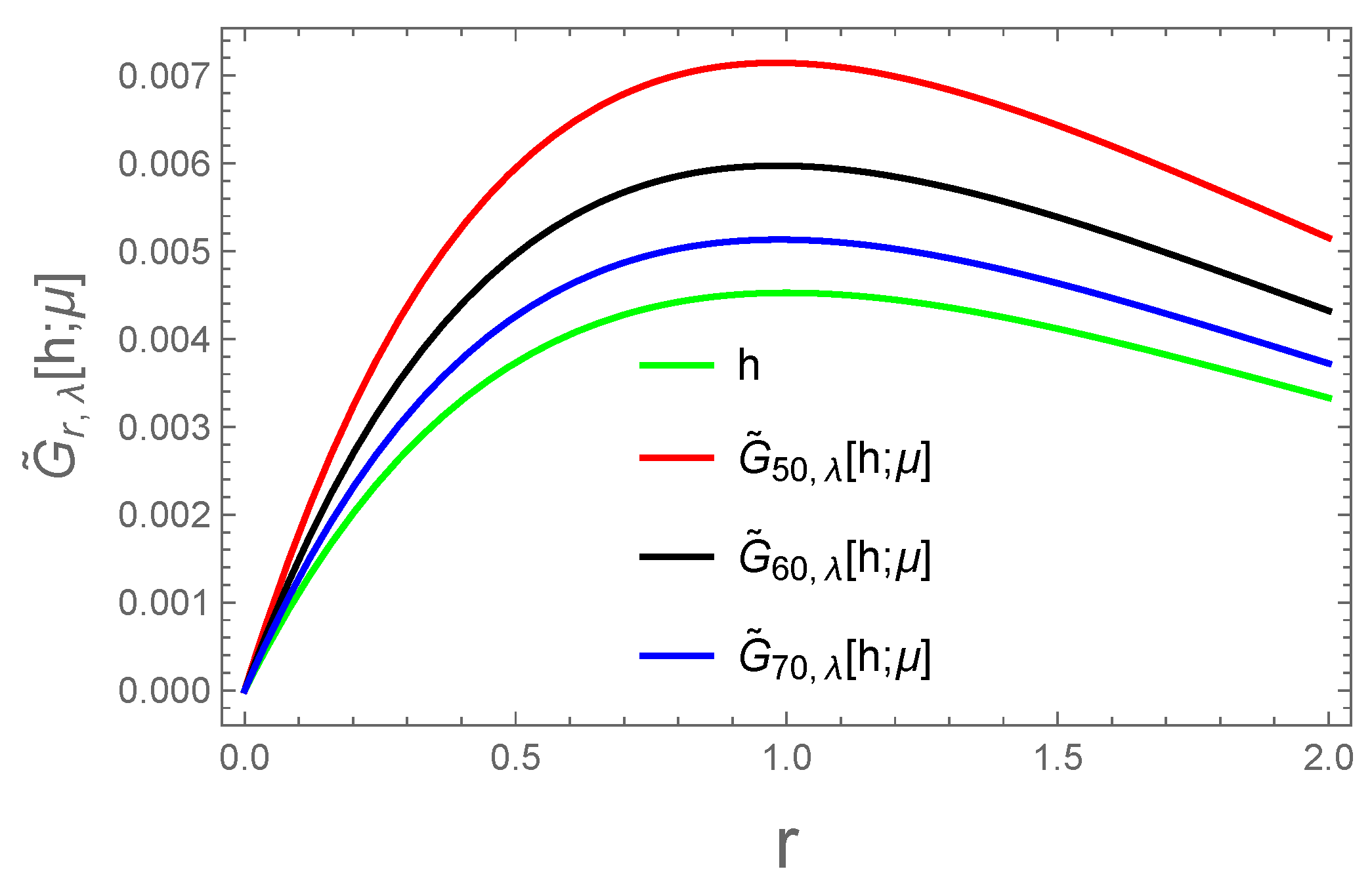
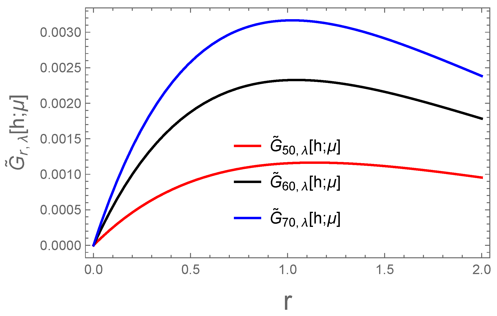
4. Graphical and Numerical Representation of ${\tilde{\mathit{G}}}_{\mathit{r},\mathit{\lambda }}(\mathit{h},\mathit{\mu })$

Here, in this part, we discuss the convergence behaviour of the operators given by (4) for the function $h\left(\mu \right)={\displaystyle \frac{\mu }{11}}{e}^{-\mu -2}.$ The numerical behaviour is discussed in

Table 1. The numerical behaviour of the operators with $\lambda =1$ for $r=50,60,70$.

u	${\tilde{\mathit{G}}}_{50,\mathit{\lambda }}(\mathit{h};\mathit{\mu })$	${\tilde{\mathit{G}}}_{60,\mathit{\lambda }}(\mathit{h};\mathit{\mu })$	${\tilde{\mathit{G}}}_{70,\mathit{\lambda }}(\mathit{h};\mathit{\mu })$
0.3	0.00437603	0.00365034	0.0031311
0.6	0.0064449	0.0053815	0.00461931
0.9	0.00711891	0.00595025	0.00511115
1.2	0.00698969	0.00584809	0.00502699
1.5	0.0064339	0.00538846	0.0046352
1.9	0.0056854	0.00476635	0.00410299

for $r=50,60,70$ for the operators of (4), with $\lambda =1,$ in terms of error formula $K_{r,\mu }(h;u)=|{\tilde{G}}_{r,\lambda }(h,\mu )-h\left(\mu \right)|.$ Moreover, a graphical depiction of the convergence and the error of the operator of (4) are given in Figure 1 and Figure 2, using $h\left(\mu \right)={\displaystyle \frac{\mu }{11}}{e}^{-\mu -2}$ and $r=50,60,70.$

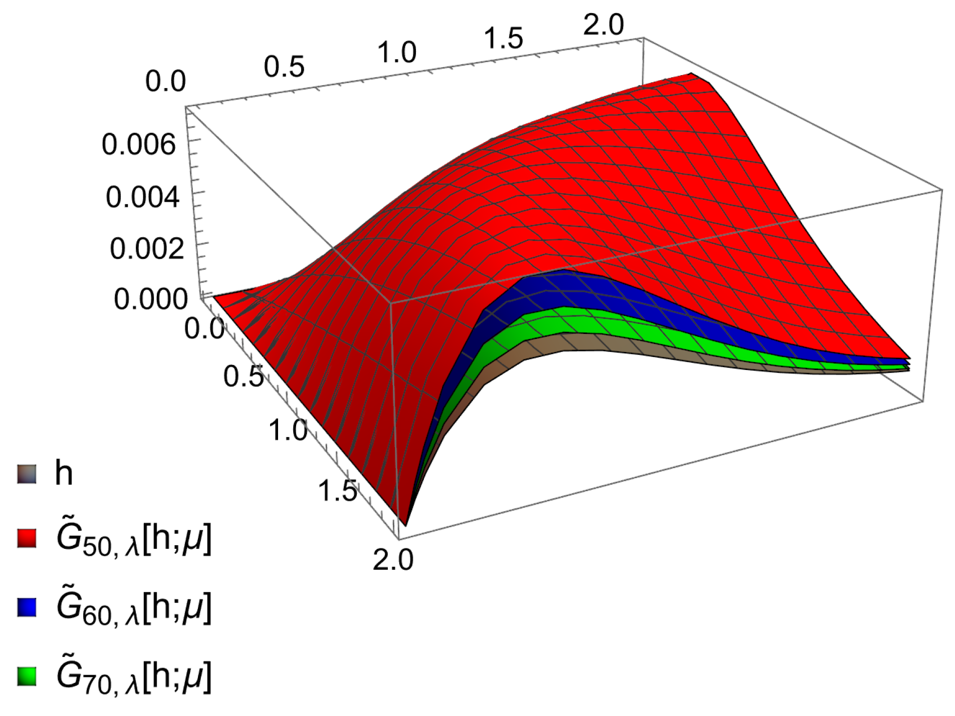
5. Bivariate of Szász–Gamma Operators via Adjoint Bernaulli Polynomials

The present section is devoted to the construction of a bivariate version of Szász–gamma-type sequences of operators via the adjoint Bernoulli polynomials of ${\tilde{G}}_{r,\lambda }(.;.)$ given by (4). Consider ${\kappa }^2=\left\{({\mu }_1,{\mu }_2):0\le {\mu }_1<\infty ,0\le {\mu }_2<\infty \right\}$ and $C\left({\kappa }^2\right)$ as a category of functions which are continuous on ${\kappa }^2$ blessed with the norm:

$$\begin{array}{c}\hfill {\parallel g\parallel }_{C\left({\kappa }^2\right)}=\underset{({\mu }_1,{\mu }_2)\in {\kappa }^2}{sup}|\hslash ({\mu }_1,{\mu }_2)|.\end{array}$$

Then, for all $\hslash \in C\left({\kappa }^2\right)$ and $r_1,r_2\in \mathbb{N}$, we introduce a bivariant version of ${\tilde{G}}_{r,\lambda }(.;.)$ given by (4) as follows:

$$\begin{array}{ccc}\hfill {\tilde{G}}_{r_1,r_2,\lambda }(\hslash ;{\mu }_1,{\mu }_2)& =& \sum _{{\nu }_1=0}^{\infty }\sum _{{\nu }_2=0}^{\infty }{g}_{{\nu }_1}\left(b_{r_1}{\mu }_1\right)g_{{\nu }_2}\left(b_{r_2}{\mu }_2\right)\hfill \\ \hfill \hspace{1em}& \times & \underset{0}{\overset{\infty }{\int }}\underset{0}{\overset{\infty }{\int }}{b}_{c_{r_1},{\nu }_1}\left({\theta }_1\right)b_{c_{r_2},{\nu }_2}\left({\theta }_2\right)\hslash ({\theta }_1,{\theta }_2)d{\theta }_{1}d{\theta }_2,\hfill \end{array}$$

where $g_{{\nu }_i}\left(b_{r_i}{\mu }_i\right)$ and $b_{c_{r_i},{\nu }_i}\left({\theta }_i\right)$ are defined in (4).

Remark 3. 

The operators introduced in Equation (23) are positive and linear operators which approximate a class of Lebesgue measurable functions in two variables.

In order to discuss the convergence rate and order of approximation, we need to find some Lemmas.

Here, we consider $p_{i,j}={\mu }_1^i{\mu }_2^j$ and ${\mathsf{\Theta }}_{i,j}^{{\mu }_1,{\mu }_2}({\theta }_1,{\theta }_2)={\eta }_{i,j}({\theta }_1,{\theta }_2)={({\theta }_1-{\mu }_1)}^i{({\theta }_2-{\mu }_2)}^j$, which, for $i,j\in \{0,1,2\}$, are the two-dimensional test functions and central moments, respectively.

Lemma 6. 

For $\hslash \in C\left({\kappa }^2\right)$ and ${\tilde{G}}_{r_1,r_2,\lambda }(.;.)$ given by Equation (23) and the test functions $p_{i,j}(.;.)$, we have

$$\begin{array}{ccc}\hfill {\tilde{G}}_{r_1,r_2,\lambda }(p_{0,0};{\mu }_1,{\mu }_2)& =& 1,\hfill \\ \hfill {\tilde{G}}_{r_1,r_2,\lambda }(p_{1,0};{\mu }_1,{\mu }_2)& =& {\displaystyle \frac{a_{r_1}}{c_{r_1}}}{\mu }_1+{\displaystyle \frac{1}{c_{r_1}}}\left({\displaystyle \frac{\lambda (e-1)+1}{e-1}}\right),\hfill \\ \hfill {\tilde{G}}_{r_1,r_2,\lambda }(p_{0,1};{\mu }_1,{\mu }_2)& =& {\displaystyle \frac{a_{r_2}}{c_{r_2}}}{\mu }_2+{\displaystyle \frac{1}{c_{r_2}}}\left({\displaystyle \frac{\lambda (e-1)+1}{e-1}}\right),\hfill \\ \hfill {\tilde{G}}_{r_1,r_2,\lambda }(p_{2,0};{\mu }_1,{\mu }_2)& =& {\displaystyle \frac{a_{r_1}^2}{c_{r_1}^2}}{\mu }_1^2+{\displaystyle \frac{a_{r_1}}{c_{r_1}^2}}(2e(\lambda +1)-2\lambda ){\mu }_1\hfill \\ \hspace{1em}& +& {\displaystyle \frac{1}{c_{r_1}^2}}\left(1+{\displaystyle \frac{2\lambda +1}{e-1}}+{\lambda }^2+\lambda \right),\hfill \\ \hfill {\tilde{G}}_{r_1,r_2,\lambda }(p_{0,2};{\mu }_1,{\mu }_2)& =& {\displaystyle \frac{a_{r_2}^2}{c_{r_2}^2}}{\mu }_2^2+{\displaystyle \frac{a_{r_1}}{c_{r_1}^2}}(2e(\lambda +1)-2\lambda ){\mu }_2\hfill \\ \hspace{1em}& +& {\displaystyle \frac{1}{c_{r_2}^2}}\left(1+{\displaystyle \frac{2\lambda +1}{e-1}}+{\lambda }^2+\lambda \right).\hfill \end{array}$$

Proof. 

To prove the above Lemma, we recall the definition of positive linear operators and Lemma (3):

$$\begin{array}{ccc}\hfill {\tilde{G}}_{r_1,r_2,\lambda }(p_{0,0};{\mu }_1,{\mu }_2)& =& {\tilde{G}}_{r_1,\lambda }(p_0;{\mu }_1){\tilde{G}}_{r_2,\lambda }(p_0;{\mu }_2),\hfill \\ \hfill {\tilde{G}}_{r_1,r_2,\lambda }(p_{1,0};{\mu }_1,{\mu }_2)& =& {\tilde{G}}_{r_1,\lambda }(p_1;{\mu }_1){\tilde{G}}_{r_2,\lambda }(p_0;{\mu }_2),\hfill \\ \hfill {\tilde{G}}_{r_1,r_2,\lambda }(p_{0,1};{\mu }_1,{\mu }_2)& =& {\tilde{G}}_{r_1,\lambda }(p_0;{\mu }_1){\tilde{G}}_{r_2,\lambda }(p_1;{\mu }_2),\hfill \\ \hfill {\tilde{G}}_{r_1,r_2,\lambda }(p_{2,0};{\mu }_1,{\mu }_2)& =& {\tilde{G}}_{r_1,\lambda }(p_2;{\mu }_1){\tilde{G}}_{r_2,\lambda }(p_0;{\mu }_2),\hfill \\ \hfill {\tilde{G}}_{r_1,r_2,\lambda }(p_{0,2};{\mu }_1,{\mu }_2)& =& {\tilde{G}}_{r_1,\lambda }(p_0;{\mu }_2){\tilde{G}}_{r_2,\lambda }(p_1;{\mu }_2).\hfill \end{array}$$

On account of the above equalities and Lemma 3, we can prove Lemma 6. □

Lemma 7. 

For ${\mathsf{\Theta }}_{i,j}={({\theta }_1-{\mu }_1)}^i{({\theta }_2-{\mu }_2)}^j$ for $i,j=0,1,2,$ then we have following equalities:

$$\begin{array}{ccc}\hfill {\tilde{G}}_{r_1,r_2,\lambda }({\mathsf{\Theta }}_{0,0};{\mu }_1,{\mu }_2)& =& 1,\hfill \\ \hfill {\tilde{G}}_{r_1,r_2,\lambda }({\mathsf{\Theta }}_{1,0};{\mu }_1,{\mu }_2)& =& {\displaystyle \frac{1}{c_{r_1}}}\left({\mu }_1+{\displaystyle \frac{\lambda (e-1)+1}{e-1}}\right),\hfill \\ \hfill {\tilde{G}}_{r_1,r_2,\lambda }({\mathsf{\Theta }}_{0,1};{\mu }_1,{\mu }_2)& =& {\displaystyle \frac{1}{c_{r_2}}}\left({\mu }_2+{\displaystyle \frac{\lambda (e-1)+1}{e-1}}\right),\hfill \\ \hfill {\tilde{G}}_{r_1,r_2,\lambda }({\mathsf{\Theta }}_{2,0};{\mu }_1,{\mu }_2)& =& {\displaystyle \frac{{\mu }_1^2}{c_{r_1}^2}}+{\displaystyle \frac{a_{r_1}}{c_{r_1}^2}}\left(2e(\lambda +1)-2\lambda -2\left({\displaystyle \frac{\lambda (e-1)+1}{e-1}}\right)\right){\mu }_1\hfill \\ \hspace{1em}& +& {\displaystyle \frac{1}{c_{r_1}^2}}\left(1+{\displaystyle \frac{2\lambda +1}{e-1}}+{\lambda }^2+\lambda \right),\hfill \\ \hfill {\tilde{G}}_{r_1,r_2,\lambda }({\mathsf{\Theta }}_{0,2};{\mu }_1,{\mu }_2)& =& {\displaystyle \frac{{\mu }_2^2}{c_{r_2}^2}}+{\displaystyle \frac{a_{r_2}}{c_{r_2}^2}}\left(2e(\lambda +1)-2\lambda -2\left({\displaystyle \frac{\lambda (e-1)+1}{e-1}}\right)\right){\mu }_2\hfill \\ \hspace{1em}& +& {\displaystyle \frac{1}{c_{r_2}^2}}\left(1+{\displaystyle \frac{2\lambda +1}{e-1}}+{\lambda }^2+\lambda \right).\hfill \end{array}$$

Proof. 

In the light of Lemma 6 and the linearity property, one can easily prove the required result. □

Definition 2. 

Consider $T_1=[0,\infty ),T_2=[0,\infty )\subset \mathbb{R}$ as given intervals and $B(T_1\times T_2)=\{\hslash :T_1\times T_2\to \mathbb{R}:\hslash asdefinedandboundedon{T}_1\times T_2\}.$ Then, for $g\in B(T_1\times T_2)$, the total modulus of continuity is defined as ${\omega }_{total}(\hslash ;·,*):C\left({\kappa }^2\right)\to \mathbb{R}$ provided that $({\tilde{\delta }}_1,{\tilde{\delta }}_2)\in T_1\times T_2$ and defined by

$${\omega }_{total}(\hslash ;{\tilde{\delta }}_1,{\tilde{\delta }}_2)=\underset{|x_1-x_1^{\prime }|\le {\tilde{\delta }}_1,|y_1-y_1^{\prime }|\le {\tilde{\delta }}_2}{sup}\left\{\right|\hslash (x_1,y_1)-\hslash (x_1^{\prime },y_1^{\prime })|:(x_1,y_1),$$

$(x_1^{\prime },y_1^{\prime })\in T_1\times T_2\},$ which is termed as the total modulus of continuity corresponding to the function ℏ.

Here, we discuss the convergence rate of the operators given by (23). To discuss the convergence rate, we revisit the following result presented by Volkov [20]:

Theorem 7. 

Let I and J be compact intervals of the real line. Let $L_{r_1,r_2}:C(I\times J)\to C(I\times J),$$(r_1,r_2)\in \mathbb{N}\times \mathbb{N}$ be linear positive operators. If

$$\begin{array}{ccc}\hfill \underset{r_1,r_2\to \infty }{lim}{L}_{r_1,r_2}\left(p_{ij}\right)& =& p_{{\mu }_1,{\mu }_2},(i,j)\in \{(0,0),(1,0),(0,1)\}\hfill \end{array}$$

and

$$\begin{array}{ccc}\hfill \underset{r_1,r_2\to \infty }{lim}{L}_{r_1,r_2}(p_{20}+p_{02})& =& p_{20}+p_{02},\hfill \end{array}$$

uniformly on $I\times J$, then the sequence $\left(L_{r_1,r_2}f\right)$ converges to ℏ uniformly on $I\times J$ for any $\hslash \in C(I\times J)$.

Theorem 8. 

Let $p_{ij}({\mu }_1,{\mu }_2)={\mu }_1^i{\mu }_2^j(0\le i+j\le 2,i,j\in \mathbb{N})$ be the test functions restricted on ${\kappa }^2$. If

$$\begin{array}{c}\hfill \underset{r_1,r_2\to \infty }{lim}{\tilde{G}}_{r_1,r_2,\lambda }(p_{ij};{\mu }_1,{\mu }_2)=p_{ij}({\mu }_1,{\mu }_2)\end{array}$$

and

$$\begin{array}{c}\hfill \underset{r_1,r_2\to \infty }{lim}{\tilde{G}}_{r_1,r_2,\lambda }(p_{20}+p_{02};{\mu }_1,{\mu }_2)=p_{20}({\mu }_1,{\mu }_2)+p_{02}({\mu }_1,{\mu }_2),\end{array}$$

uniformly on ${\kappa }^2$, then

$$\begin{array}{c}\hfill \underset{r_1,r_2\to \infty }{lim}{\tilde{G}}_{r_1,r_2,\lambda }(\hslash ;{\mu }_1,{\mu }_2)=\hslash ({\mu }_1,{\mu }_2),\end{array}$$

uniformly for all $\hslash \in C\left({\kappa }^2\right)$.

Proof. 

In view of Lemma 6, it is evident for $i=j=0$ that

$$\begin{array}{c}\hfill \underset{r_1,r_2\to \infty }{lim}{\tilde{G}}_{r_1,r_2,\lambda }(p_{00};{\mu }_1,{\mu }_2)=p_{00}({\mu }_1,{\mu }_2).\end{array}$$

For $i=1$, $j=0$, we obtain

$$\begin{array}{ccc}\hfill \underset{r_1,r_2\to \infty }{lim}{\tilde{G}}_{r_1,r_2,\lambda }(p_{10};{\mu }_1,{\mu }_2)& =& {\mu }_1,\hfill \\ \hfill \underset{r_1,r_2\to \infty }{lim}{\tilde{G}}_{r_1,r_2,\lambda }(p_{10};{\mu }_1,{\mu }_2)& =& p_{10}({\mu }_1,{\mu }_2).\hfill \end{array}$$

Similarly,

$$\begin{array}{ccc}\hfill \underset{r_1,r_2\to \infty }{lim}{\tilde{G}}_{r_1,r_2,\lambda }(p_{01};{\mu }_1,{\mu }_2)& =& {\mu }_2,\hfill \\ \hfill \underset{r_1,r_2\to \infty }{lim}{\tilde{G}}_{r_1,r_2,\lambda }(p_{01};{\mu }_1,{\mu }_2)& =& p_{01}({\mu }_1,{\mu }_2),\hfill \end{array}$$

and, in the light of Lemma (6), we obtain

$$\begin{array}{ccc}\hfill \underset{r_1,r_2\to \infty }{lim}{\tilde{G}}_{r_1,r_2,\lambda }(p_{20}+p_{02};{\mu }_1,{\mu }_2)& =& {\mu }_1^2+{\mu }_2^2,\hfill \\ \hspace{1em}& =& p_{20}({\mu }_1,{\mu }_2)+p_{02}({\mu }_1,{\mu }_2).\hfill \end{array}$$

In this direction, Theorem 7 and Theorem 8 are easily proved. □

In the last result, we deal with the approximation order of the sequence of operators of ${\tilde{G}}_{r_1,r_2,\lambda }(.;.)$ given by (23) as follows:

Theorem 9 

([21]). Let $L:C\left({\kappa }^2\right)\to B\left({\kappa }^2\right)$ be a linear positive operator. For any $\hslash \in C\left({\kappa }^2\right)$, any $(z_1,z_2)\in {\kappa }^2$ and any ${\tilde{\delta }}_1,{\tilde{\delta }}_2>0$, the inequality

$$\begin{array}{ccc}\hfill |(L\hslash )(z_1,z_2)-\hslash (z_1,z_2)|& \le & |L{p}_{0,0}(z_1,z_2)-1\left|\right|\hslash (z_1,z_2)|+[L{p}_{0,0}(z_1,z_2)\hfill \\ \hspace{1em}& +& {\tilde{\delta }}_1^{-1}\sqrt{L{p}_{0,0}(z_1,z_2){\left(L(·-z_1)\right)}^2(z_1,z_2)}\hfill \\ \hspace{1em}& +& {\tilde{\delta }}_2^{-1}\sqrt{L{p}_{0,0}(z_1,z_2){\left(L(\ast -z_2)\right)}^2(z_1,z_2)}\hfill \end{array}$$

$$\begin{array}{ccc}\hspace{1em}& +& {\tilde{\delta }}_1^{-1}{\tilde{\delta }}_2^{-1}\sqrt{{\left(L{p}_{0,0}\right)}^2(z_1,z_2){\left(L(·-z_1)\right)}^2(z_1,z_2){\left(L(\ast -z_2)\right)}^2(z_1,z_2)}]\hfill \\ \hspace{1em}& \times & {\omega }_{total}(\hslash ;{\tilde{\delta }}_1,{\tilde{\delta }}_2),\hfill \end{array}$$

holds.

Theorem 10. 

For $\hslash \in C\left({\kappa }^2\right)$ and $({\mu }_1,{\mu }_2)\in {\kappa }^2$, $(r_1,r_2)\in \mathbb{N}\times \mathbb{N}$ and ${\tilde{\delta }}_1,{\tilde{\delta }}_2>0$, one has

$$\begin{array}{c}\hfill |{\tilde{G}}_{r_1,r_2,\lambda }(\hslash ;{\mu }_1,{\mu }_2)-\hslash ({\mu }_1,{\mu }_2)|\le 4{\omega }_{total}(\hslash ;{\tilde{\delta }}_1,{\tilde{\delta }}_2),\end{array}$$

where ${\tilde{\delta }}_1=\sqrt{{\tilde{G}}_{r_1,r_2,\lambda }\left({\mathsf{\Theta }}_{2,0};{\mu }_1,{\mu }_2\right)}$ and ${\tilde{\delta }}_2=\sqrt{{\tilde{G}}_{r_1,r_2,\lambda }\left({\mathsf{\Theta }}_{0,2};{\mu }_1,{\mu }_2)\right)}$.

Proof. 

From Theorem 9, we have

$$\begin{array}{ccc}\hspace{1em}& .& |({\tilde{G}}_{r_1,r_2,\lambda }\hslash )({\mu }_1,{\mu }_2)-\hslash ({\mu }_1,{\mu }_2)|\hfill \\ \hspace{1em}& \le & [1++{\tilde{\delta }}_1^{-1}\sqrt{{\tilde{G}}_{r_1,r_2,\lambda }\left({\mathsf{\Theta }}_{2,0};{\mu }_1,{\mu }_2\right)}\hfill \\ \hspace{1em}& +& {\tilde{\delta }}_2^{-1}\sqrt{{\tilde{G}}_{r_1,r_2,\lambda }\left({\mathsf{\Theta }}_{0,2};{\mu }_1,{\mu }_2\right)}\hfill \\ \hspace{1em}& +& {\tilde{\delta }}_1^{-1}{\tilde{\delta }}_2^{-1}\sqrt{{\tilde{G}}_{r_1,r_2,\lambda }\left({\mathsf{\Theta }}_{2,0};{\mu }_1,{\mu }_2\right){\tilde{G}}_{r_1,r_2,\lambda }\left(({\mathsf{\Theta }}_{0,2};{\mu }_1,{\mu }_2\right)}]\hfill \\ \hspace{1em}& \times & {\omega }_{total}(f;{\tilde{\delta }}_1,{\tilde{\delta }}_2).\hfill \end{array}$$

Selecting ${\tilde{\delta }}_1=\sqrt{{\tilde{G}}_{r_1,r_2,\lambda }\left({\mathsf{\Theta }}_{2,0};{\mu }_1,{\mu }_2\right)}$ and ${\tilde{\delta }}_2=\sqrt{{\tilde{G}}_{r_1,r_2,\lambda }\left({\mathsf{\Theta }}_{0,2};{\mu }_1,{\mu }_2)\right)}$, we arrive at the required result. □

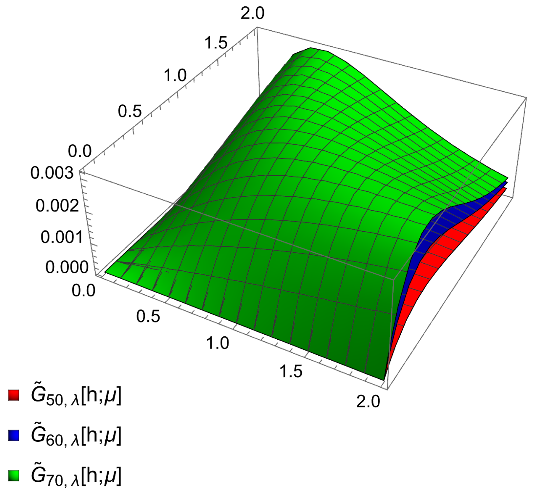
6. Bivariate Graphical Representation

In this section, we study the two-dimensional approximation behaviour of the given operator (23) with the help of a graphical and numerical approach for $r_1,r_2=50,60,70$ and $\lambda =1$ for the newly constructed operator ${\tilde{G}}_{r_1,r_2,\lambda }(h,\mu ).$ It can be observed in the table and figure given below, for the different set of parameters $\lambda =1$, that the operator ${\tilde{G}}_{r_1,r_2,\lambda }(h,\mu )$ converges uniformly to the function ${\displaystyle \frac{{\mu }_1.{\mu }_2}{11}}{e}^{-{\mu }_1{\mu }_2}$. Furthermore, using error formula $K_{r_1,r_2}(h;{\mu }_1,{\mu }_2)=|{\tilde{G}}_{r_1,r_2,\lambda }(h;{\mu }_1,{\mu }_2)-h({\mu }_1,{\mu }_2)|$, the error of operator (23) is as shown in Figure 3 and Figure 4.

7. Conclusions

This research work introduces a new connection of adjoint Bernoulli polynomials and a gamma function as a new sequence of linear positive operators denoted by ${\left\{{\tilde{G}}_{r,\lambda }(.;.)\right\}}_1^{\infty }$. Further, the convergence properties of these sequences of operators, i.e., ${\left\{{\tilde{G}}_{r,\lambda }(.;.)\right\}}_1^{\infty }$, are investigated in various functional spaces with the aid of the Korovkin theorem, Voronovskaja-type theorem, first order of modulus of continuity, second order of modulus of continuity, Peetre’s K-functional, Lipschitz condition, etc. In the last section, we extend our research for the bivariate case of these sequences of operators, and their uniform rate of approximation and order of approximation are investigated in different functional spaces. These sequences of operators have advantages.

• This research work connects two fields of research (special function research and operators theory).
• These sequence operators are capable of approximating in a wider class of functions, i.e., the class of Lebesgue measurable functions.
• These sequences of operators also provide better approximation results in terms of Chlodowsky.

References

1. Bernstein, S.N. Démonstration du théorème de Weierstrass fondée sur le calcul de probabilités. Commun. Soc. Math. Kharkow. 1913, 13, 1–2. [Google Scholar]
2. Weierstrass, K. Über die analytische Darstellbarkeit sogenannter willkürlicher Functionen einer reellen Veränderlichen. Sitzungsberichte Königlich Preußischen Akad. Wiss. Berl. 1885, 2, 633–639. [Google Scholar]
3. Aslan, R. Rate of approximation of blending type modified univariate and bivariate λ-Schurer-Kantorovich operators. Kuwait J. Sci. 2024, 51, 100168. [Google Scholar] [CrossRef]
4. Leinartas, E.K.; Shishkina, O.A. The discrete analogue of the Newton-Leibniz formula in the problem of summation over simple lattice points. J. Sib. Fed. Univ. Math. Phys. 2019, 12, 503–508. [Google Scholar] [CrossRef]
5. Mohiuddine, S.A.; Acar, T.; Alotaibi, A. Construction of a new family of Bernstein-Kantorovich operators. Math. Methods Appl. Sci. 2017, 40, 7749–7759. [Google Scholar] [CrossRef]
6. Rao, N.; Malik, P.; Rani, M. Blending type Approximations by Kantorovich variant of α-Baskakov operator. Palest. J. Math. 2022, 11, 402–413. [Google Scholar]
7. Rao, N.; Gulia, K. On two dimensional Chlodowsky-Szász operators via Sheffer Polynomials. Palest. J. Math. 2023, 12, 521–531. [Google Scholar]
8. Appell, P.P. Sur une class de polynômes. In Annales Scientifiques de l’É cole Normale Supérieure. Norm Supér; Société Matheématique de France: Paris, France, 1880; Volume 2, pp. 119–144. [Google Scholar]
9. Natalini, P.; Ricci, E. Adjoint Appell–Euler and first kind Appell–Bernoulli’s polynomials. Appl. Appl. Math. 2019, 14, 1112–1122. [Google Scholar]
10. Lyapin, A.P.; Leinartas, E.K.; Grigoriev, A.A. Summation of functions and polynomial solutions to a multidimensional difference equation. J. Sib. Fed. Univ. Math. Phys. 2023, 16, 153–161. [Google Scholar]
11. Costabile, F.A.; Gualtieri, M.I.; Napoli, A. Some results on generalized Szasz operators involving Sheffer polynomials. J. Comput. Appl. Math. 2018, 337, 244–255. [Google Scholar] [CrossRef]
12. Costabile, F.A. An Introduction to Modern Umbral Calculus De Gryter. In Studies in Mathematics; De Gruyter: Berlin, Germany; Boston, MA, USA, 2019; Volume 72. [Google Scholar] [CrossRef]
13. Costabile, F.A.; Gualtieri, M.I.; Capizzano, S.S. Asyptotic expansion and extrapolation for Bernstein polynomials. BIT Num. Math. 1998, 36, 676–687. [Google Scholar] [CrossRef]
14. Costabile, F.A.; Gualtieri, M.I.; Capizzano, S.S. Asyptotic expansion and extrapolation for positive linear operators. Ann Univ. Ferrara ViiXiV 2000, 45, 431–442. [Google Scholar]
15. Yilmaz, M.M. Rate of convergence by Kantorovich type operators involving adjoint Bernoulli’s polynomials. Publ. L’Institut Mathématique Nouv. Série Tome 2023, 114, 51–62. [Google Scholar]
16. Devore, R.A.; Lorentz, G.G. Constructive Approximation; Springer: Berlin/Heidelberg, Germany, 1993. [Google Scholar]
17. Altomare, F.; Campiti, M. Korovkin-type approximation theory and its applications. De Gruyter Ser. Stud. Math. 1994, 17, 266–274. [Google Scholar]
18. Özarslan, M.A.; Aktuğlu, H. Local approximation for certain King type operators. Filomat 2013, 27, 173–181. [Google Scholar] [CrossRef]
19. Lenze, B. On Lipschitz type maximal functions and their smoothness spaces. Nederl. Akad. Indag. Math. 1988, 50, 53–63. [Google Scholar] [CrossRef]
20. Volkov, V.I. On the convergence of sequences of linear positive operators in the space of continuous functions of two variables. Dokl. Akad. Nauk SSSR (NS) 1957, 115, 17–19. (In Russian) [Google Scholar]
21. Stancu, F. Approximarca Funcṭiilor de Douăşi mai Multe Vsrabile Prin ṣiruri de Operatori Liniari ṣi Positivi. Ph.D. Thesis, Cluj-Napoca, Romania, 1984. [Google Scholar]
Figure 1. Convergence of operator G ˜ r , λ ( h , μ ) for r = 50 , 60 , 70 .
Mathematics 12 03645 g001
Figure 2. Error approximation K r , λ ( h ; μ ) = | G ˜ r , λ ( h , μ ) h ( μ ) | .
Mathematics 12 03645 g002
Figure 3. Convergence of operator G ˜ r 1 , r 2 , λ ( . ; . ) for r = 50 , 60 , 70 .
Mathematics 12 03645 g003
Figure 4. Error approximation K r 1 , r 2 ( h ; μ 1 , μ 2 ) = | G ˜ r 1 , r 2 , λ ( h ; μ 1 , μ 2 ) h ( μ 1 , μ 2 ) | .
Mathematics 12 03645 g004