Article

Analytical Models of Experimental Artefacts in an Ill-Posed Nonlinear ODE System

School of Engineering, Zurich University of Applied Sciences (ZHAW), 8400 Winterthur, Switzerland
*
Author to whom correspondence should be addressed.
Mathematics 2024, 12(23), 3675; https://doi.org/10.3390/math12233675 (registering DOI)
Submission received: 21 October 2024 / Revised: 17 November 2024 / Accepted: 21 November 2024 / Published: 24 November 2024
(This article belongs to the Section Mathematical Physics)

Abstract

:
We discuss different approaches for the analytical description of a mechanical system used in control theory, aiming at the analytical modelling of experimental artefacts observed in the implementation of ideal searched trajectories. Starting from an established analytical solution, we develop an alternative analytical model for this solution with minimal deviations and then extend this starting point to a more flexible toolbox that incorporates a variety of phenomena that typically occur in real implementations of this mechanical system, thus providing an important step towards bridging the gap between theoretical models and experimental reality.

1. Introduction

The mechanical–dynamic system cubli, schematically depicted in Figure 1, is an important example of an inverted pendulum and has served as a use case for various research topics, ranging from control theory to mechanical engineering and numerical analysis.
The system has two degrees of freedom, the rotation of the rigid body around its corner and the rotation of the flywheel, described by the two coordinates ϕ 1 and ϕ 2 , as depicted in Figure 1; in addition, there is an external moment function f ( t ) which is theoretically given, but which turns out to be rather difficult to implement experimentally. The movement of the system can be imagined schematically as depicted in Figure 2; precisely, we consider a lift-up process where the system is required to be moved from an initial to a final configuration, which are both prescribed, thereby using a theoretically given moment function. This, however, turns out to be rather difficult to exactly implement in an experimental situation, which is one of the starting points for our study.
For the history of the model and its related research endeavours, we refer to the vast literature (see, e.g., [1,2,3,4] for cubli and [5,6] for inverted pendulums in general); the latest advances in the investigation of the model from a robotics perspective can be found in [7]. Note that besides serving as a benchmark case for novel research approaches, e.g., as control-theory reference models (see the overviews provided by [8,9]), it is also used as a tool for engineering education. For some recent advances on the cubli research in general, we refer to the overview provided in our previous study [10].
Less common are attempts at a precise understanding of the model from the viewpoint of a mathematical analysis, which is mainly due to the difficulties in analytically solving the ODE system associated with the model. In [10], we presented an analytical solution of the model based on the assumption that the moment function had a certain special structure, which seemed to be unmotivated, but which turned out to lead to a result which closely resembled what one expects to see from an ideal implementation of the sought-for moment trajectory.
However, it then turned out that whereas the angle trajectory indeed was very well described by the analytical solution of our previous work, the moment trajectory considerably differed from what was expected ideally and correspondingly modelled by the previous solution; this discrepancy between an ideal trajectory and its inconsistent implementation results is an example of an experimental distortion, a phenomenon which is well known in various application settings.
This phenomenon of a relatively stable angle trajectory connected to a considerable variety of moment trajectories shows, on the one hand, a certain robustness of the angle trajectory with respect to perturbations of the moment function input but also demonstrates the need to have a flexible analytical toolbox for the analytical understanding of various possible moment function trajectories. The purpose of the present paper therefore is to develop a framework for the analytical description of a great variety of moment trajectories under the side condition of leaving the angle trajectory largely unchanged.
Dealing with artefacts and corruptions in experimental data nowadays is a vast research field [11,12,13,14,15,16,17,18,19,20,21,22,23,24]. To begin with a more detailed description of these attempts at artefact removal, the occurrence of artefacts is a frequent obstacle in MRI and CT images; various strategies (classical and machine learning-based) for dealing with artefacts in these domains are discussed in the overview articles [11] (for MRI) and [12] (for CT), respectively. Furthermore, many of these works are dealing with artefacts in EEG signals: The review article [13] discusses a variety of methods such as regression-based methods, wavelet transforms, BSS (blind signal separation), EMD (empirical mode decomposition), filtering-based or sparse decomposition methods, as well as hybrid approaches combining several of the aforementioned methods. Bayesian deep learning is then discussed in [14] as an artefact-removal method, and [17] establishes a cost-efficient “online” (i.e., real-time) method for handling EEG artefacts. Various approaches for dealing with artefacts in TMS (transcranial magnetic stimulation)-EEG signals are discussed in [16]; in [21], the authors propose the usage of transformer architectures, one of the most recent machine learning paradigms which has already shown considerable successes in other domains. Another type of signals which requires artefacts to be dealt with are DBS (deep brain stimulation) data; for this domain, various approaches are proposed in [15] (irregular sampling methods), [18] (dealing with high-frequency stimulation artefacts hindering the analysability of underlying neural signals), or [19] (combining singular value decomposition and normalized adaptive filtering). Yet other application domains are considered in [20] (artefacts in electrical microstimulation data), focusing on a trade-off between accuracy and computational complexity, and [22] (artefacts in electrically evoked frequency-following responses). Finally, the review articles [23,24] provide surveys of deep learning-based methods for general anomaly detection in industrial time series, which can be employed in a variety of application contexts.
In most cases, the intent is to “clean up” the distorted experimental data with smart algorithms which are trained with uncorrupted (partially synthetic) data. These algorithms are often based on deep learning architectures, whose power has led to impressive successes, but whose complexity makes it often difficult to fundamentally understand their predictive power, which is especially crucial when one tries to apply them to problems whose data they have not been trained on. For a discussion of the general concept of artefacts, we refer to [25].
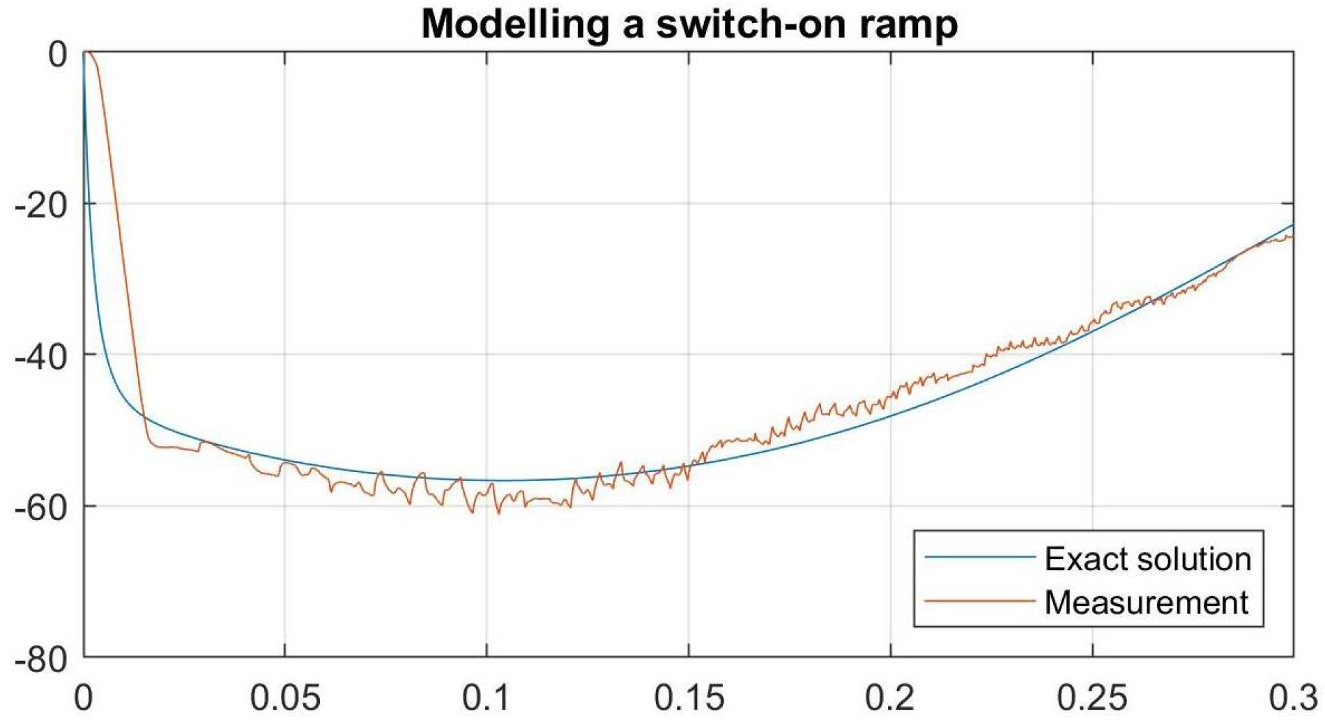
On the other hand, approaches directed towards the analytical description of experimental artefacts are scarcely reported in the literature [26,27,28]. Here, we follow this conceptually different approach of aiming for exact analytical solutions describing the various types of distortions encountered in their experimental implementation; thus we do not intend to resolve the distortions but to develop exact analytical models for their description, which are intended to be also flexible enough to deal with distortion types which have not been encountered yet. The starting point of our analysis is the above-mentioned observation that the angle trajectories seem to exhibit a certain robustness with respect to perturbed moment trajectories. We then develop various analytical tools for obtaining solutions of our system, which all lead to a relatively similar angle trajectory but are able to model a various number of these considerably different moment trajectories, such as the one depicted in Figure 3, where one of our solutions is depicted together with a (slightly smoothened) measurement of such an implemented moment trajectory.
Sticking to the usage of analytical methods in the era of ever-increasing computing power may seem awkward; in our previous paper [10], we explained that even under the present circumstances, the search for analytical solutions has various advantages, ranging from their educational value to the structural insights into a given problem, which they are able to give to a much larger extent than brute-force computational approaches; besides the references mentioned therein, the quest for analytical solutions of various problems continues to be a field of active research, see e.g., the recent papers [29,30,31,32]. In particular, the idea of trying to explain experimental artefacts with exact mathematical models, instead of trying to ignore/repair/correct them, seems to be rather unusual. Starting from the analytical solution obtained previously, we thus start with developing an alternative model for the same solution with minimal deviations and then extend this starting point to a more flexible toolbox incorporating a variety of the phenomena which are usually encountered, thus providing a significant step in bridging the gap between theoretical models and experimental reality.
Overview of the paper In Section 2, we formulate the problem mathematically, we review our past solution strategy of the problem and explain its limitations, resp. the necessity of further investigations, and we outline our solution strategy. In Section 3, we explain and implement a first version of our new approach of analytically modelling the problem with a more flexible and extensible toolbox, thereby always assessing its numerical accuracy. In Section 4, we then extend our previous approach into various directions, with the goal of analytically modelling the aforementioned distortions occurring in the laboratory reality of implementing a given moment trajectory. Finally, in Section 5, we discuss the significance of our results and give some hints on further research directions.

2. Mathematical Model and Experimental Reality

As can be seen from Figure 1, the dynamics of the system is described by two angle variables ϕ 1 and ϕ 2 . Here, we reduce the discussion on the ODE for the first angle variable ϕ 1 , since its dynamics can be considered independently of ϕ 2 , and the dynamics of ϕ 2 can easily be recovered once the dynamics of ϕ 1 is known. The dynamical system for the variable ϕ 1 π 4 is given by the ODE
ϕ ¨ ( t ) = α · sin ( ϕ ( t ) ) f ( t )
together with the boundary conditions
ϕ ( 0 ) = π 4 , ϕ ( τ ) = 0 , ϕ ˙ ( 0 ) = 0 , ϕ ˙ ( τ ) = 0
at t = 0 and at the ending time t = τ of the lift-up procedure, as well as the additional condition
0 τ f ( t ) d t = ω β
Since a second-order ODE in general admits only two additional conditions, the system is clearly overdetermined with the 5 conditions listed in (2) and (3), if all parameters α , β , ω , τ , as well as the moment function f ( t ) are treated as given. Note that from the formulation (3), it might seem strange to treat β and ω as separate parameters and not to introduce a new parameter for the quantity ω β ; however, this is because in an extended model also encompassing the second angle ϕ 2 , the parameter ω has the physical meaning of initial velocity of ϕ 2 . In this paper, we exclusively focus on the ODE for ϕ 1 (which is independent of ϕ 2 ), and therefore the ODE for ϕ 2 is omitted.
In our previous work [10], we implemented a “forward strategy”, which consisted in finding closed solutions of the problem in a special case of the function f ( t ) , namely, when f ( t ) can be written as a trigonometric polynomial of the first solution function ϕ ( t ) , i.e., in the form f ( t ) = u · sin ( ϕ 1 ( t ) ) + v · cos ( ϕ 1 ( t ) ) . In this case, the solution can be found in terms of elliptic functions, and the parameters u and v are determined by the boundary conditions (2) on ϕ , as well as τ by the condition (3). In this ansatz, we thus cope with the ill-posedness by introducing two additional parameters through the special form for f ( t ) , and the analytical difficulties are overcome by assuming f ( t ) to be a trigonometric polynomial in ϕ ( t ) .
Precisely, in [10], we proved the following theorem:
Theorem 1.
Let α , β , ω > 0 be fixed. Then, there exist constants u , v , τ R depending only on α , β , ω such that the initial-boundary integral value problem consisting of the ODE
ϕ ¨ ( t ) = α · sin ( ϕ ( t ) ) ( u · sin ( ϕ ( t ) ) + v · cos ( ϕ ( t ) ) ) ,
the initial-boundary conditions
ϕ ( 0 ) = π 4 , ϕ ( τ ) = 0 , ϕ ˙ ( 0 ) = 0 , ϕ ˙ ( τ ) = 0
and the integral condition
0 τ ( u · sin ( ϕ ( t ) ) + v · cos ( ϕ ( t ) ) ) d t = ω β
admits a unique solution. It is given by
ϕ ( t ) = 2 · arcsin sn κ 2 · t κ 0 sin 2 π 16 π 8
where κ 0 and κ 2 also depend only on α , β , ω . Here, sn ( u | m ) is one of the Jacobian elliptic functions which are reviewed in Appendix A of [10].
The constants appearing in the preceding result are computed explicitly; we refer to [10], since they are of limited relevance in the present context.
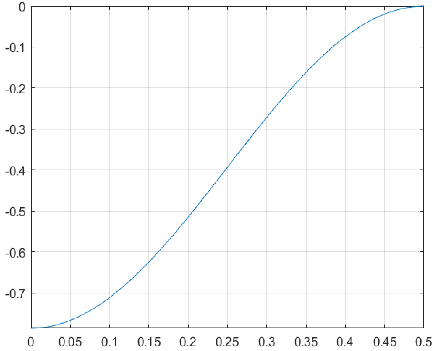
In the sequel, we choose the parameters α , β , ω such that we arrive at τ = 0.5 . For such a choice, the functions ϕ ( t ) and f ( t ) on the interval [ 0 , τ ] are plotted in Figure 4 and Figure 5.
Even though the forward analysis yields a result which is surprisingly similar to what one expects to observe in the experiment (which justifies the assumptions on ϕ ( t ) made above in order to make the problem amenable to elliptic functions), its weakness is the lack of stability and robustness with respect to changes in the parameters of the system, and more importantly its lack of flexibility to incorporate other moment map trajectories arising from experimental artefacts and inaccuracies in the implementation.
Moreover, implementing the moment map in the laboratory has made it clear that the angle trajectory is relatively robust with respect to changes in the moment map trajectory. Our solution model using elliptic functions is not sufficiently flexible to model this robustness, namely, this rather intricate dependence between moment and angle trajectories.
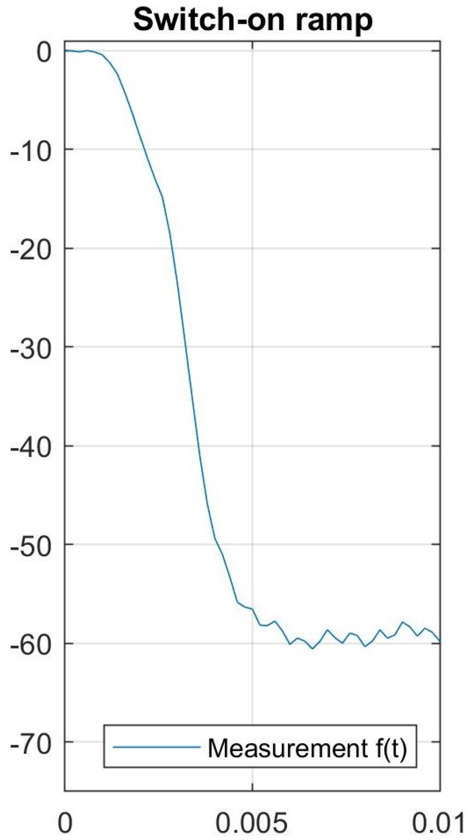
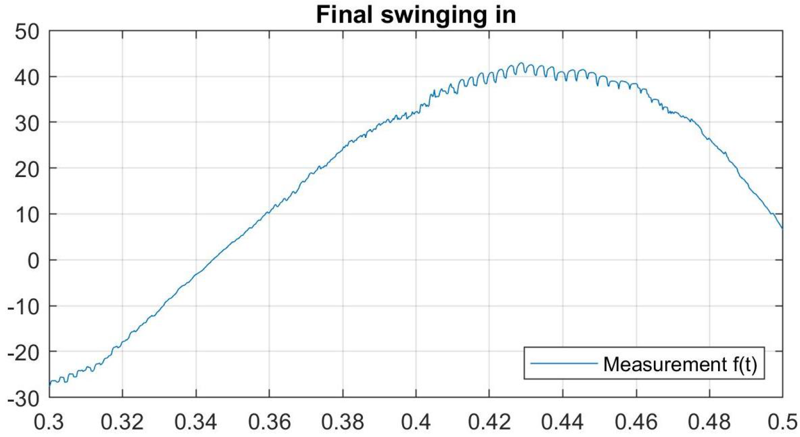
In particular, in the experiment one often encounters switch-on ramps and final swing-ins of the types depicted in Figure 6 and Figure 7:
These ramps and swing-outs/swing-ins should be compared to the ideal moment trajectory modelled with our previous approach and depicted in Figure 5. The possibility of obtaining relatively unchanged angle trajectories with considerably distorted moment trajectories can intuitively be explained by a relatively simple perturbation calculation, as we now first show.
For a given solution ϕ 0 ( t ) of the cubli problem with associated moment function f 0 ( t ) , let
ϕ ϵ ( t ) = ϕ 0 ( t ) + ϵ · δ ( t )
be an angle trajectory which is perturbed by the additional term ϵ · δ ( t ) , which is chosen such that ϕ ϵ ( t ) continues to fulfil the boundary conditions (2) of the problem. The corresponding moment trajectory is then given by
f ϵ ( t ) = α · sin ( ϕ ϵ ( t ) ) ϕ ¨ ϵ ( t )
and hence, by considering a Taylor expansion in ϵ
f ϵ ( t ) = α · sin ( ϕ 0 ( t ) ) + α · cos ( ϕ 0 ( t ) ) · δ ( t ) · ϵ + o ( ϵ 2 ) ϕ ¨ 0 ( t ) ϵ · δ ¨ ( t ) ,
and
f ϵ ( t ) = f 0 ( t ) + α · cos ( ϕ 0 ( t ) ) · δ ( t ) · ϵ + o ( ϵ 2 ) ϵ · δ ¨ ( t ) .
The fact that ϵ was chosen small enough such that the perturbation ϵ · δ ( t ) of the angle trajectory can be neglected for practical purposes does not imply that f 0 ( t ) cannot be substantially distorted by ϵ · δ ¨ ( t ) .
Our basic strategy in dealing with these issues is to use a “backward” strategy, i.e., we first focus on the boundary conditions (2) for ϕ ( t ) , and fulfil these conditions by functions which are as simple as possible, i.e., polynomials of the lowest possible degree. In this ansatz, we thus do not solve the ODE but “solve” the boundary conditions and use the ODE to determine the moment function f ( t ) . Having obtained ϕ ( t ) in this way, we compute f ( t ) by (1). Again, condition (3) is used to determine τ . Focusing primarily on the boundary conditions thus has the advantage that these conditions can be easily extended by additional constraints or satisfied by different types of basic functions, which then allows us to choose those functions leading to a result which best satisfies the physical aspects of the problem.
As already mentioned after Theorem 1, in applications, the parameters are typically chosen such that the time constant τ takes a certain value. We usually choose the parameters such that τ takes the realistic value τ = 0.5 , on which basis the plots of Figure 4 and Figure 5 were created. This choice is possible by Theorem 2 through the situational adaptation of ω , which is technically easy to realize in laboratory environments. In the sequel, ϕ 0 ( t ) is the exact solution of the cubli problem to the normed moment trajectory f 0 ( t ) according to Theorem 1.

3. Backward Analysis: Principle

In order to overcome the problems arising from the forward approach of Theorem 1 discussed in the previous section, in this section, we follow a different method, as already outlined towards the end of the previous section: we try to fulfil the given boundary conditions for ϕ 1 ( t ) by some given class of functions, and then compute f ( t ) . In this ansatz, (1) is no longer considered a differential equation for ϕ 1 ( t ) but rather an (algebraic) equation for f ( t ) . This may seem like a strange way to treat a boundary value problem, but we justify it from its successes in modelling the experimentally observed behaviour, in particular concerning various moment map trajectories.
Theorem 2.
Let α , β , ω > 0 be fixed, and let g ( t ) be any C 2 -function satisfying the boundary conditions
g ( 0 ) = 1 , g ( 1 ) = 0 , g ˙ ( 0 ) = 0 , g ˙ ( 1 ) = 0 .
as well as
0 1 sin π 4 g ( s ) d s 0
Then there exists a unique τ > 0 such that the function
ϕ ( t ) = π 4 g t τ
satisfies the initial-boundary integral value problem (1)–(3) for the moment function
f ( t ) = α · sin ( ϕ ( t ) ) ϕ ¨ ( t ) .
Proof. 
It follows from the boundary conditions (5) of g ( t ) that for any fixed value of τ > 0 , the function ϕ ( t ) , as defined by (7), satisfies the conditions (2). If for this angle function ϕ ( t ) , the moment function f ( t ) is then defined by (8), it is obvious that the ODE (1) is satisfied. It remains to check that there is a unique choice of τ such that (3) is satisfied as well.
We first address the uniqueness of τ and thereby assume the validity of the integral condition (3), which by (1) can be rewritten as
0 τ α sin ( ϕ ( t ) ) ϕ ¨ ( t ) d t = ω β .
Plugging (7) into (9), we obtain, using ϕ ˙ ( 0 ) = ϕ ˙ ( τ ) = 0 ,
ω β = 0 τ α sin ( ϕ ( t ) ) ϕ ¨ ( t ) d t = 0 τ α sin ( ϕ ( t ) ) d t = α 0 τ sin π 4 · g t τ d t = α τ 0 1 sin π 4 · g ( s ) d s = : I .
By assumption (6), we can solve (10) for τ and obtain
τ = 1 I · ω α β
This shows the uniqueness of τ . Conversely, if τ is defined by
τ = 1 0 1 sin π 4 · g ( s ) d s · ω α β
the above reasoning shows that (9) and therefore (3) are satisfied. This concludes the proof of Theorem 2. □
As mentioned above, the purpose of Theorem 2 is to provide a toolbox for solutions of the cubli problem whose corresponding moment function describes various aspects of what we observe in real implementations of the experiment as results instead of what was sought for. Note that throughout this paper, τ takes the value τ = 0.5 , and that ω is adapted to the context of the respective situation by using the Formula (11) for choosing ω such that τ = 0.5 .

4. Backward Analysis: Examples

4.1. Approximating the Ideal Solution by Hermite Splines

Third-order Hermite splines The first (and most straightforward) application of Theorem 2 is to use third-order Hermite splines to satisfy (5), namely, to consider the polynomial
g 00 ( t ) = 2 t 3 3 t 2 + 1
which is (by the theory of Hermite splines) the unique third-order polynomial satisfying the boundary conditions (5), and it clearly satisfies (6). The associated solution function
ϕ 1 ( t ) = π 4 g 00 t τ
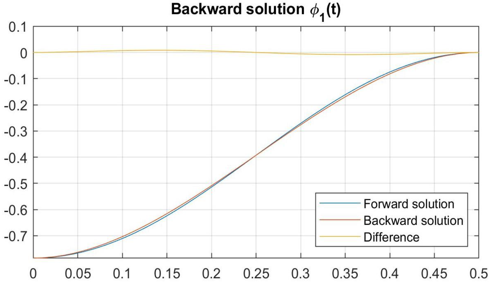
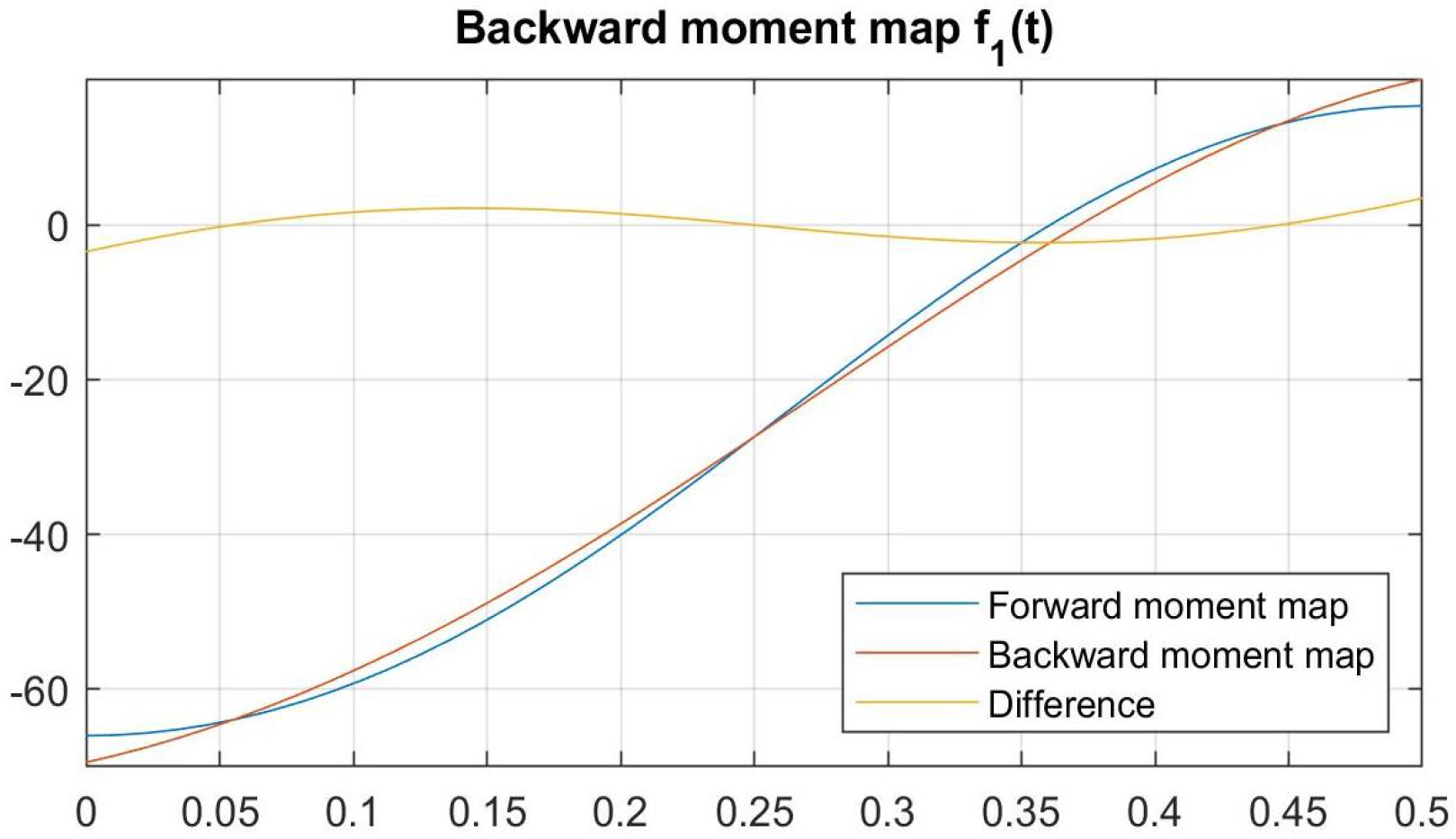
then solves the cubli problem by Theorem 2. A comparison of the angle and moment trajectories corresponding to the forward solution (4) and the new backward solution (14) is given in Figure 8 and Figure 9 below; note that as in the previous section, we choose the parameters α , β , ω such that we obtain for τ the value τ = 0.5 . More precisely, the values of α and β are kept fixed, whereas ω is then chosen according to (11) such that we obtain τ = 0.5 . For reference purposes, we mention that this amounts to approximately the values
α = 71.6040 , β = 6.8407 , ω = 90.13789
(this can be seen by noting that the integral defined in (10) has the numerical value I 0.368487 , and then plugging this into (12) for the values (15) of α , β , ω ).
The numerical proximity between a polynomial and a highly transcendental function visible in Figure 8, involving inverse Jacobian elliptic functions, seems striking, and the corresponding moment maps, visible in Figure 9, show an almost equivalent similarity. This strong similarity is the starting point for our refined approaches in the next section: we intend to keep the proximity of our angle trajectories to the forward solution, while at the same time gaining more flexibility in the moment trajectories, with the goal of modelling the aforementioned artefacts in the implementation of ideal moment trajectories.
To improve the approximation of the forward solution with elliptic functions of the problem, we now extend our solution approaches into various directions, with the goal of improving the quality of the approximation, but nevertheless keeping the relative simplicity of the functions used for the approximation.
Fifth-order Hermite splines A natural refinement of the solution approach (14) is to use fifth-order Hermite splines of the form
h ˜ 00 ( t ) = 1 10 t 3 + 15 t 4 6 t 5 h ˜ 20 ( t ) = 1 2 t 2 3 2 t 3 + 3 2 t 4 1 2 t 5 h ˜ 21 ( t ) = 1 2 t 3 t 4 + 1 2 t 5
Except for h ˜ 00 ( 0 ) = 1 , they all have zeros at t = 0 and t = 1 , and the same applies to their derivatives. In addition to (16), we consider the scaled versions
h 00 ( t ) = π 4 · h ˜ 00 t τ , h 20 ( t ) = h ˜ 20 t τ u n d h 21 ( t ) = h ˜ 21 t τ .
Now, we consider a solution approach of the form
ϕ 2 ( t ) = h 00 ( t ) + a 20 · h 20 ( t ) + a 21 · h 21 ( t ) .
By Theorem 2, with the boundary conditions satisfied by the functions (16) and their rescaling in (17), the function ϕ 2 ( t ) , as given by (18), is a solution of the original cubli problem (1)–(3) for the moment function
f ( t ) = α · sin ( ϕ 2 ( t ) ) ϕ ¨ 2 ( t ) .
To determine optimal values of the parameters a 20 and a 21 in (18), we minimize the L 2 -norm of the distance of ϕ 2 to ϕ 0 , where ϕ 0 is the forward solution (4) given by Theorem 1. Note that by (18),
ϕ 2 ( t ) ϕ 0 ( t ) = ( h 00 ( t ) ϕ 0 ( t ) ) + a 20 · h 20 ( t ) + a 21 · h 21 ( t ) .
Writing the (squared) L 2 -norm | ϕ 2 ( t ) ϕ 0 ( t ) | 2 2 of the difference to the forward solution as a function of a 20 and a 21 , we have
I ( a 20 , a 21 ) = | ϕ 2 ( t ) ϕ 0 ( t ) | 2 2 = 0 τ ( ϕ 2 ( t ) ϕ 0 ( t ) ) 2 d t
Plugging (19) into this expression, we obtain
I ( a 20 , a 21 ) = I u u + 2 · I u v · a 20 + 2 · I u w · a 21 + 2 · I v w · a 20 · a 21 + I v v · a 20 2 + I w w · a 21 2
for
I u u = 0 τ ( h 00 ( t ) ϕ 0 ( t ) ) 2 d t I v v = 0 τ h 20 ( t ) 2 d t I w w = 0 τ h 21 ( t ) 2 d t I u v = 0 τ ( h 00 ( t ) ϕ 0 ( t ) ) · h 20 ( t ) d t I u w = 0 τ ( h 00 ( t ) ϕ 0 ( t ) ) · h 21 ( t ) d t I v w = 0 τ h 20 ( t ) · h 21 ( t ) d t
Minimizing I ( a 20 , a 21 ) as given by (20) is an elementary analytical problem with a unique solution. Note that the parameter values have again been chosen such that we arrive at τ = 0.5 .
A numerical evaluation of the solution leads to the values
a 20 min 3.7186 , a 21 min 3.7186 , I min 0.000065
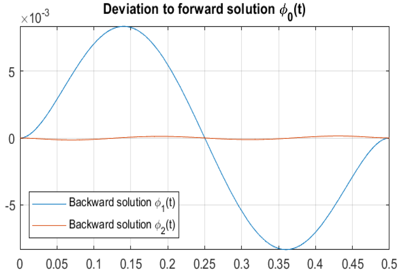
Figure 10 shows the forward solution (4), the solution (7) using third-order Hermite splines, and the solution (18) with the minimal values a 20 min , a 21 min of the coefficients just computed; note that Figure 10 should be considered as an extension of Figure 8. The improvement in deviation from the forward solution can be more clearly seen in Figure 11, where the deviations of the third-order and of the fifth-order Hermite spline solution from the forward solution given by Jacobian elliptic functions are plotted.
The moment function f 2 ( t ) corresponding to the fifth-order solution ϕ 2 ( t ) is obtained by plugging ϕ 2 ( t ) , given by (18), into the formula for f ( t ) , i.e.,
f 2 ( t ) = α · sin ( ϕ 2 ( t ) ) ϕ ¨ 2 ( t ) .
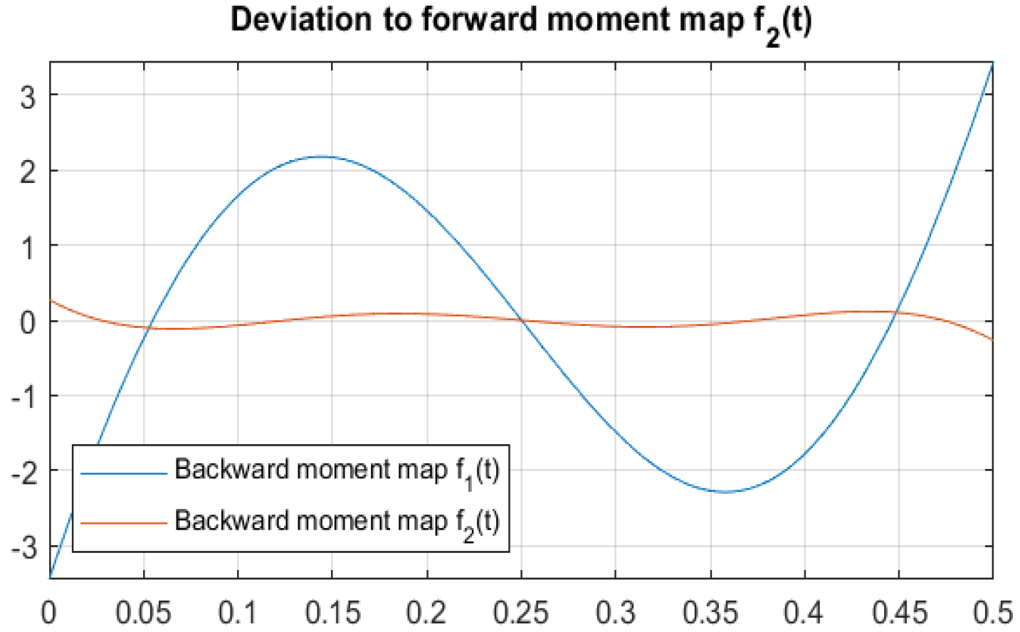
It is depicted in Figure 12; similarly to Figure 10, the moment function resulting from the fifth-order Hermite spline solution can be barely distinguished from the moment function resulting from the forward solution given by Jacobian elliptic functions; in Figure 13, we show the deviation plot corresponding to Figure 11.
Altogether, we note that the forward solution by Jacobian elliptic functions does barely deviate from the solution by fifth-order Hermite splines; it seems clear that this approximation quality could be increased even more by invoking higher-order Hermite splines. However, this would not lead us to the second goal of this paper, namely, to analytically model moment functions which do not correspond to the (theoretically expected) moment function given by the forward solution, as, e.g., shown in Figure 5. Such artefacts have been presented in Figure 6 and Figure 7. Therefore, we now no longer focus on creating even closer approximations to the forward solution ϕ 0 ( t ) but on creating solutions of the problem which remain relatively close to ϕ 0 ( t ) but have a considerable difference in their moment map trajectories.

4.2. Investigating the Dependence Between Angle and Moment Trajectories

Let
ϕ 12 ( t ) = ϕ 2 ( t ) + b 20 · h 20 ( t ) + b 20 · h 21 ( t )
be an arbitrary angle trajectory with associated moment trajectory f 12 ( t ) , where ϕ 2 ( t ) is the solution (18) considered above, and h 20 and h 21 continue to be the fifth-order Hermite splines considered above, cf. (16) and (17). Using the boundary conditions of h 20 ( t ) and h 21 ( t ) , it can easily be seen by Theorem 2 that the function (23) solves the cubli problem for any values of b 20 and b 21 .
In order to determine the L 2 -distance between ϕ 12 ( t ) and the forward solution ϕ 0 ( t ) , we can—with negligible inaccuracies, cf. Figure 10—use the L 2 -distance between ϕ 12 ( t ) and ϕ 2 ( t ) , and we thereby obtain
| ϕ 12 ( t ) ϕ 2 ( t ) | 2 2 = 0 τ ( ( ϕ 2 ( t ) + b 20 · h 20 ( t ) + b 20 · h 21 ( t ) ) ( ϕ 2 ( t ) + a 20 · h 20 ( t ) + a 21 · h 21 ( t ) ) ) 2 d t = 0 τ ( δ 20 · h 20 ( t ) + δ 21 · h 21 ( t ) ) 2 d t = : I ( δ 20 , δ 21 )
with
δ 20 = b 20 a 20 and δ 21 = b 21 a 21 ,
and we therefore obtain
I ( δ 20 , δ 21 ) = I v v · δ 20 2 + 2 · I v w · δ 20 · δ 21 + I w w · δ 21 2
with I v v , I w w , and I v w being defined as above, cf. (21), and the numerical values
I v v = I w w 0.0000541 , I v w = 0.0000451 .
In eigencoordinates, the quadratic form I ( δ 20 , δ 21 ) takes the form
I ( δ ˜ 20 , δ ˜ 21 ) = 0.00000902 · δ ˜ 20 2 + 0.0000992 · δ ˜ 21 2 ,
and the corresponding eigendirections are
1 2 , 1 2 and 1 2 , 1 2 .
The “most dramatic” choice
( b 20 , b 21 ) = ( a 20 , a 21 ) 1 0.00000902 · ϵ · 1 2 , 1 2
hence creates a distance ϵ of ϕ 12 ( t ) to ϕ 0 ( t ) . With ϵ = 0.005 , we obtain
( b 20 , b 21 ) ( 2.60545 , 2.60545 )
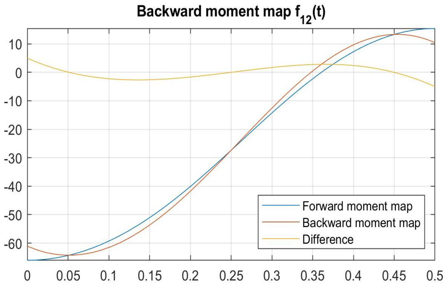
and we obtain the barely changed angle trajectory depicted in Figure 14 but the considerably changed moment trajectory depicted in Figure 15:
Note in particular the “swinging out” and “swinging in” at the beginning and at the end of the time period under consideration, respectively.
If we accept an accuracy of ϵ = 0.01 , the initial swinging out and final swinging in become even more distinct, as Figure 16 and Figure 17 show:
These preliminary results concerning the modelling of these additional phenomena mainly arising in the moment trajectories, which do not seem to have a considerable influence on the angle trajectory, are motivating the additional models which we present in the sequel.

4.3. Analytical Models of Experimental Artefacts

Initial swinging out: This type of swinging out and in at both ends of the process, which we already to some extent modelled with the previous rather simple approach involving fifth-order Hermite splines, is a phenomenon which occurs in many technical applications. To improve the analytical modelling of such phenomena, we consider an improved perturbation of the previously determined fifth-order Hermite solution ϕ 2 ( t ) by ϕ 2 ( t ) + θ ( t ) , which leads to the associated moment function
f θ ( t ) = α · sin ( ϕ 2 ( t ) + θ ( t ) ) ϕ ¨ 2 ( t ) θ ¨ ( t )
Note that θ ( t ) has to be chosen such that ϕ 2 ( t ) + θ ( t ) continues to satisfy the boundary conditions (2) of the original problem. If, e.g., p ( t ) is a polynomial of the form
p ( t ) = t m 1 ( t 1 ) m 2 , m 1 , m 2 2
then p ( t ) has vanishing function and derivative values at t = 0 and t = 1 . According to Theorem 2, for θ ( t ) = c · p t τ and any linear combination of the Hermite splines h 20 ( t ) and h 21 ( t ) already considered previously, the function
ϕ 13 ( t ) = ϕ 2 ( t ) + b 20 · h 20 ( t ) + b 21 · h 21 ( t ) + θ 13 ( t )
then solves the cubli problem. In modelling the initial swinging out of real-world implementations of f 0 ( t ) , the ansatz
p 1 ( t ) = t 2 · ( t 1 ) 6
and θ ( t ) = 4 · p t τ turn out to be a sound choice. Minimizing the L 2 -distance between ϕ 13 ( t ) and ϕ 0 ( t ) leads to the optimal parameter values
b 20 = 3.2448 and b 21 = 1.6783
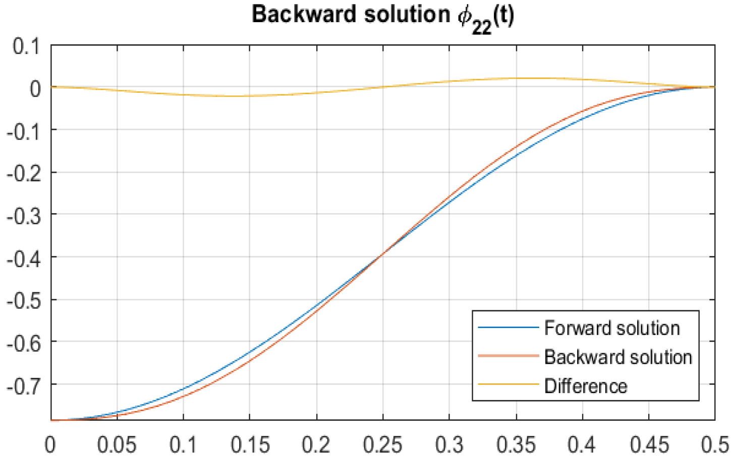
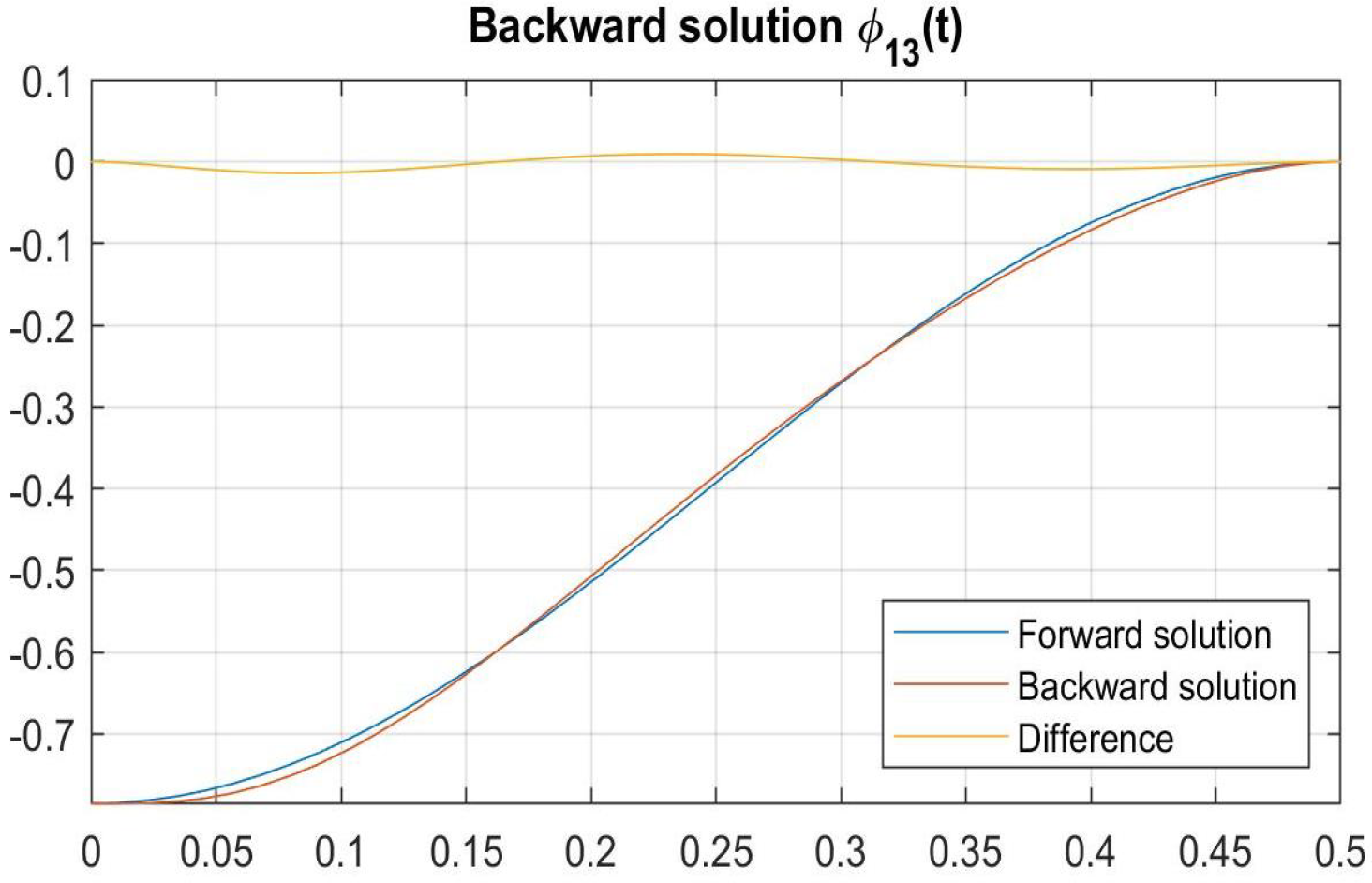
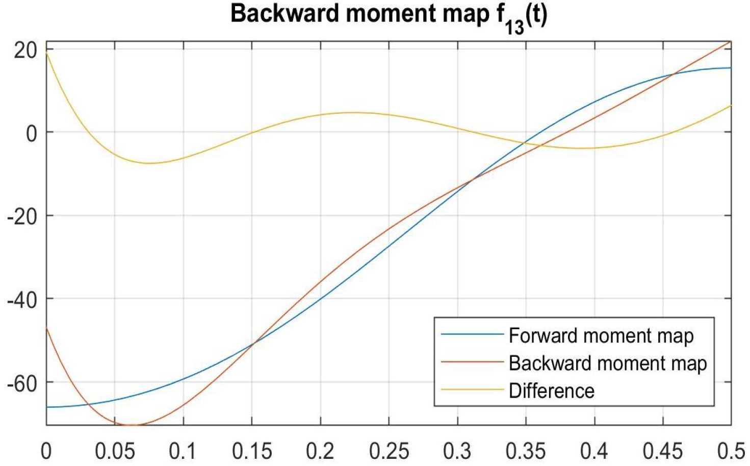
in (25). The associated moment trajectory f 13 ( t ) then exhibits a realistic model of this initial swinging-out process. The L 2 -norm
| ϕ 13 ( t ) ϕ 0 ( t ) | 2 0.005
shows that the additional term θ 13 barely influences the angle trajectory, as can be seen in Figure 18; on the other hand, the moment trajectory now shows a clear initial oscillation, as Figure 19 shows:
Final swinging in: In modelling the final swinging in of real-world implementations of f 0 ( t ) , the ansatz
ϕ 23 ( t ) = ϕ 2 ( t ) + b 20 · h 20 ( t ) + b 21 · h 21 ( t ) + θ 23 ( t )
with θ 23 ( t ) = 3 · p 1 t τ for
p 1 ( t ) = t 6 · ( t 1 ) 2
turns out to be a good choice. Minimizing the L 2 -distance between ϕ 23 ( t ) and ϕ 0 ( t ) leads to the optimal parameter values
b 20 = 2.4336 and b 21 = 0.00395 ,
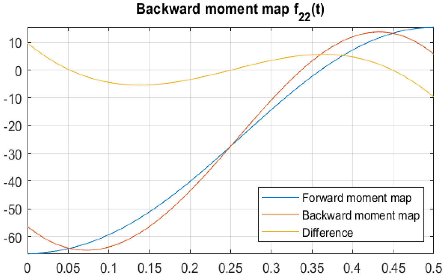
together with the associated moment trajectory f 13 ( t ) . Again it follows from our general framework result, Theorem 2, that ϕ 23 ( t ) , as given by (26) for any choice of b 20 and b 21 and any choice of p 1 of the type (24), satisfies the cubli problem. The L 2 -norm
| ϕ 13 ( t ) ϕ 0 ( t ) | 2 0.005
then shows that the additional term θ 13 barely influences the angle trajectory, as can be seen in Figure 20. On the other hand, the moment trajectory now shows a clear final swinging in, as Figure 21 shows:
Initial ramp: The previous calculations suggest for the modelling of the initial ramp an ansatz containing a function with an initially very large but then rapidly decaying derivative near the origin. Such a behaviour can be modelled with rational functions, which motivates the approach which we take in the sequel. Consider the functions
r 0 ( t ) = t 2 · ( t τ ) 4 ( m · t + 1 ) n r 1 ( t ) = t 3 · ( t τ ) 3 r 2 ( t ) = t 4 · ( t τ ) 2
i.e., a rational function and two polynomials. Here, m and n are two form parameters, which are in the sequel selected to be m = 200 and n = 1 ; note that the denominator of the rational function r 0 ( t ) has been kept as simple as possible, i.e., linear, and the pole of r 0 ( t ) very close to zero in order to obtain a sufficient steepness near the origin. The selection of these values depends on the goal of the modelling; this is an example of the flexibility of our approach.
Since all of these functions, as well as their derivatives, vanish at t = 0 and t = τ , the linear combination
ϕ 3 ( t ) = ϕ 2 ( t ) + a 0 · r 0 ( t ) + a 1 · r 1 ( t ) + a 2 · r 2 ( t )
is a solution of the cubli problem, again according to our general framework result, Theorem 2, with the associated moment function computed by (8). Note that in (27), the function ϕ 2 ( t ) is again the solution (18) obtained above with fifth-order Hermite splines with the optimal parameter values (22). Altogether, our choices of the functions r 0 ( t ) , r 1 ( t ) , and r 2 ( t ) in the ansatz (27) are motivated by the desire to obtain a realistic analytical description of the artefacts observed in the experimental implementation of sought-for moment trajectories with functions which are as simple as possible.
To choose the parameters a 0 , a 1 , and a 2 in (27), we first require that f 3 ( 0 ) = 0 , which ensures the ramp-type behaviour of f ( t ) , and then, in addition, that the L 2 -distance of ϕ 3 ( t ) to ϕ 2 ( t ) be minimized. The first condition can be satisfied by setting
a 0 = α 2 + ϕ ¨ 2 ( 0 ) r ¨ 0 ( 0 )
The minimization of the L 2 -distance of ϕ 3 ( t ) to ϕ 2 ( t ) amounts to minimizing
| ϕ 3 ( t ) ϕ 2 ( t ) | 2 2 = | a 0 · r 0 ( t ) + a 1 · r 1 ( t ) + a 2 · r 2 ( t ) | 2 2
The quantity (28) can then be rephrased as
I ( a 1 , a 2 ) = I u u + 2 · I u v · a 1 + 2 · I u w · a 2 + 2 · I v w · a 1 · a 2 + I v v · a 1 2 + I w w · a 2 2
for
I u u = 0 τ ( a 0 · r 0 ( t ) ) 2 d t , I v v = 0 τ ( r 1 ( t ) ) 2 d t , I w w = 0 τ ( r 2 ( t ) ) 2 d t
and, cf. the similar quantities used in (21) for the previous minimization,
I u v = 0 τ a 0 · r 0 ( t ) · r 1 ( t ) d t , I u w = 0 τ a 0 · r 0 ( t ) · r 2 ( t ) d t , I v w = 0 τ r 1 ( t ) · r 2 ( t ) d t .
The minimization of the L 2 -norm of the distance of ϕ 3 to ϕ 2 turns out to be an elementary minimization problem of the functional (29) with solutions
a 1 0.0599 and a 2 = 0.0261 ,
which corresponds to the minimal norm
| ϕ 3 ( t ) ϕ 2 ( t ) | 2 0.0025
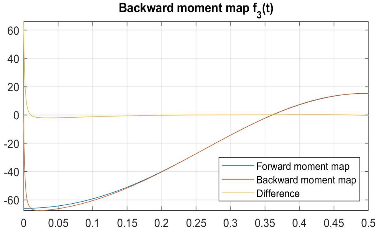
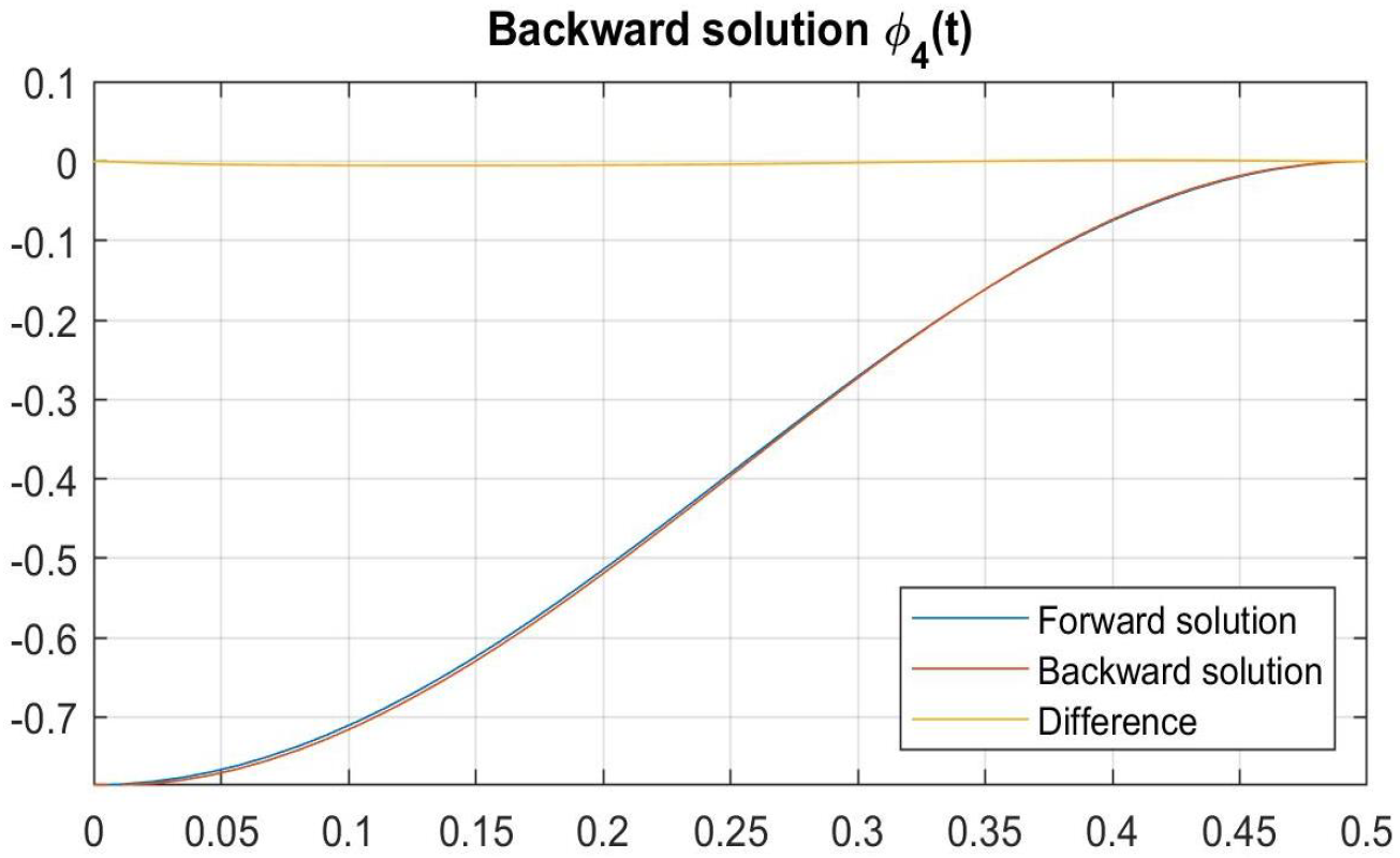
Figure 22 confirms the proximity of ϕ 2 and ϕ 3 ; on the other hand, the normed moment trajectory is dramatically changed in the initial time period, as the following Figure 23 shows:
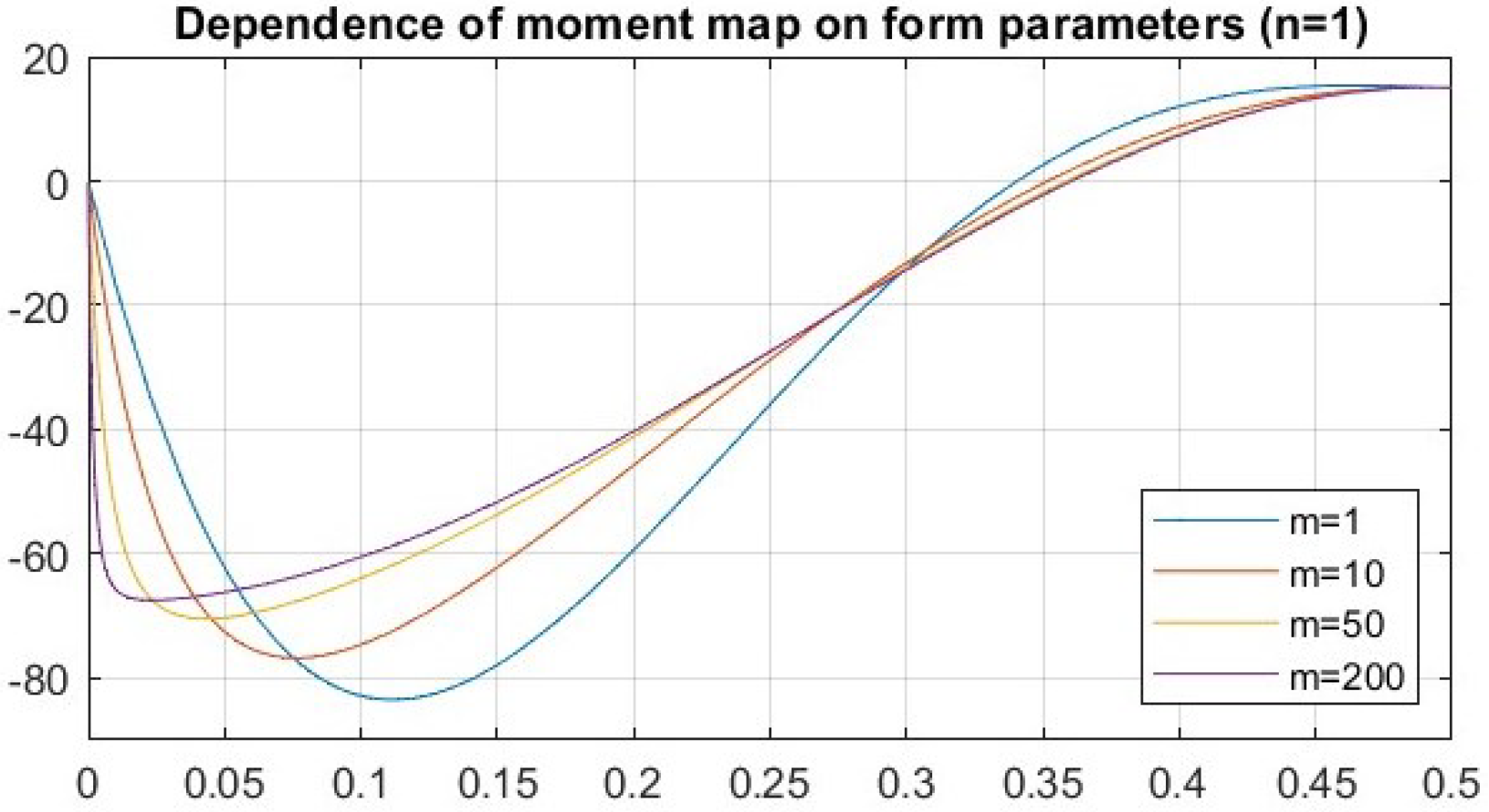
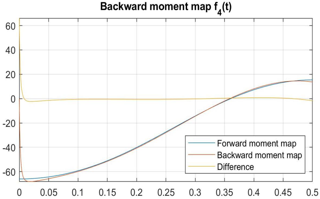
This moment trajectory is directed towards modelling the switch-on procedure of the experimental implementation with its initial inertia. As already indicated before, this explains the condition f 3 ( 0 ) = 0 , whereas the initial overshoot of f 3 ( t ) is typical for this situation. The dependence of the moment trajectory on the form parameters is demonstrated by the various possibilities depicted in Figure 24:
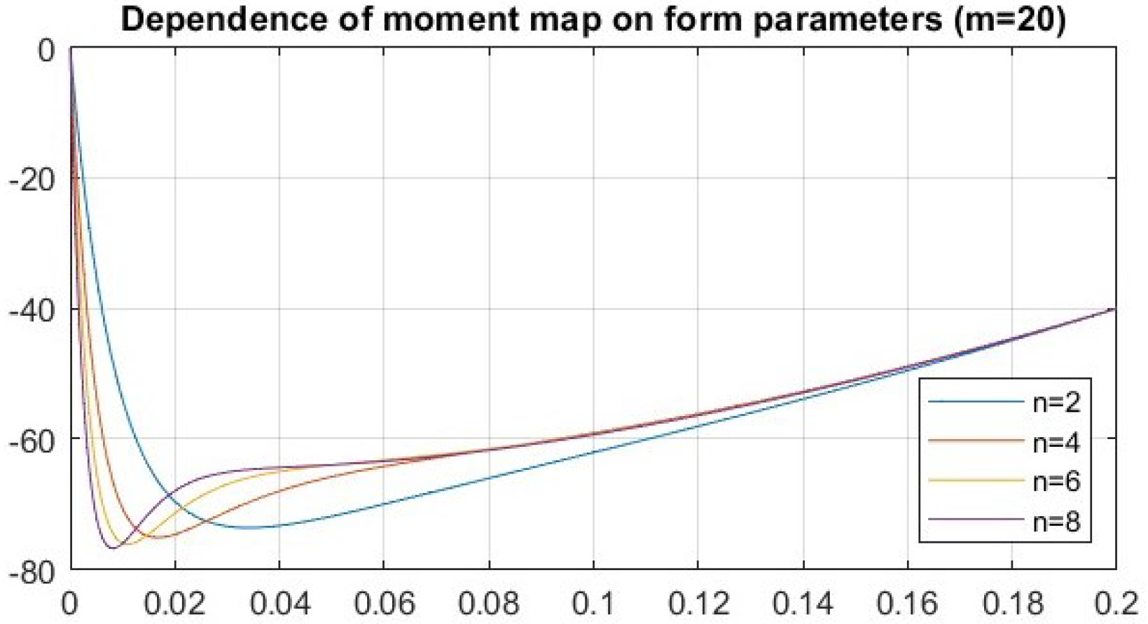
As Figure 24 shows, the form parameter m describes the steepness of the switch-on ramp and to a certain, extend the initial overshooting. On the other hand, the form parameter n describes the qualitative nature of the initial overshooting, which we demonstrate in Figure 25:
Blending all elements: Typically, a real trajectory contains an initial switch-on ramp, an initial swinging in, and a final swinging back. For the modelling of such a real behaviour, we can select a linear combination of ϕ 3 (for the initial ramp), ϕ 13 (for the initial swinging in), and ϕ 23 (for the final swinging back). Note that this option of linearly combining the various solution models exists notwithstanding the nonlinear nature of the cubli problem. It can rather be explained by the fact that the deviations from the ideal behaviour are mainly stemming from a term with a second derivative, which is a linear term.
We thus consider the linear combination
ϕ 4 ( t ) = c 3 · ϕ 3 ( t ) + c 13 · ϕ 13 ( t ) + c 23 · ϕ 23 ( t ) ,
where the weights c 3 , c 13 , c 23 should satisfy the additional constraints
c 3 + c 12 + c 13 = 1
as well as
c 3 · ϕ ¨ 3 ( 0 ) + c 13 · ϕ ¨ 13 ( 0 ) + c 23 · ϕ ¨ 23 ( 0 ) = α 2
By the first additional condition (30), we are ensuring that ϕ 4 ( t ) satisfies the cubli boundary conditions, whereas the second additional constraint (31) ensures that the ramp condition f ( 0 ) = 0 is satisfied. The weights are finally chosen such that the L 2 -norm
| ϕ 4 ( t ) ϕ 2 ( t ) | 2
is minimized. The minimization of the L 2 -norm of the distance of ϕ 4 to ϕ 2 under the above-mentioned additional constraints turns out to be a classical optimization problem, which can be solved by a Lagrangian technique, with the result
c 3 1.0305 c 13 0.0897 c 23 0.0532 .
The corresponding minimal norm
| ϕ 4 ( t ) ϕ 2 ( t ) | 2 0.0024
indicates a substantial closeness of ϕ 4 and ϕ 0 , which is confirmed by the corresponding plots of the angle trajectory, see the following Figure 26; in addition, Figure 27 shows that the moment trajectory f 4 ( x ) models the real moment trajectory convincingly:
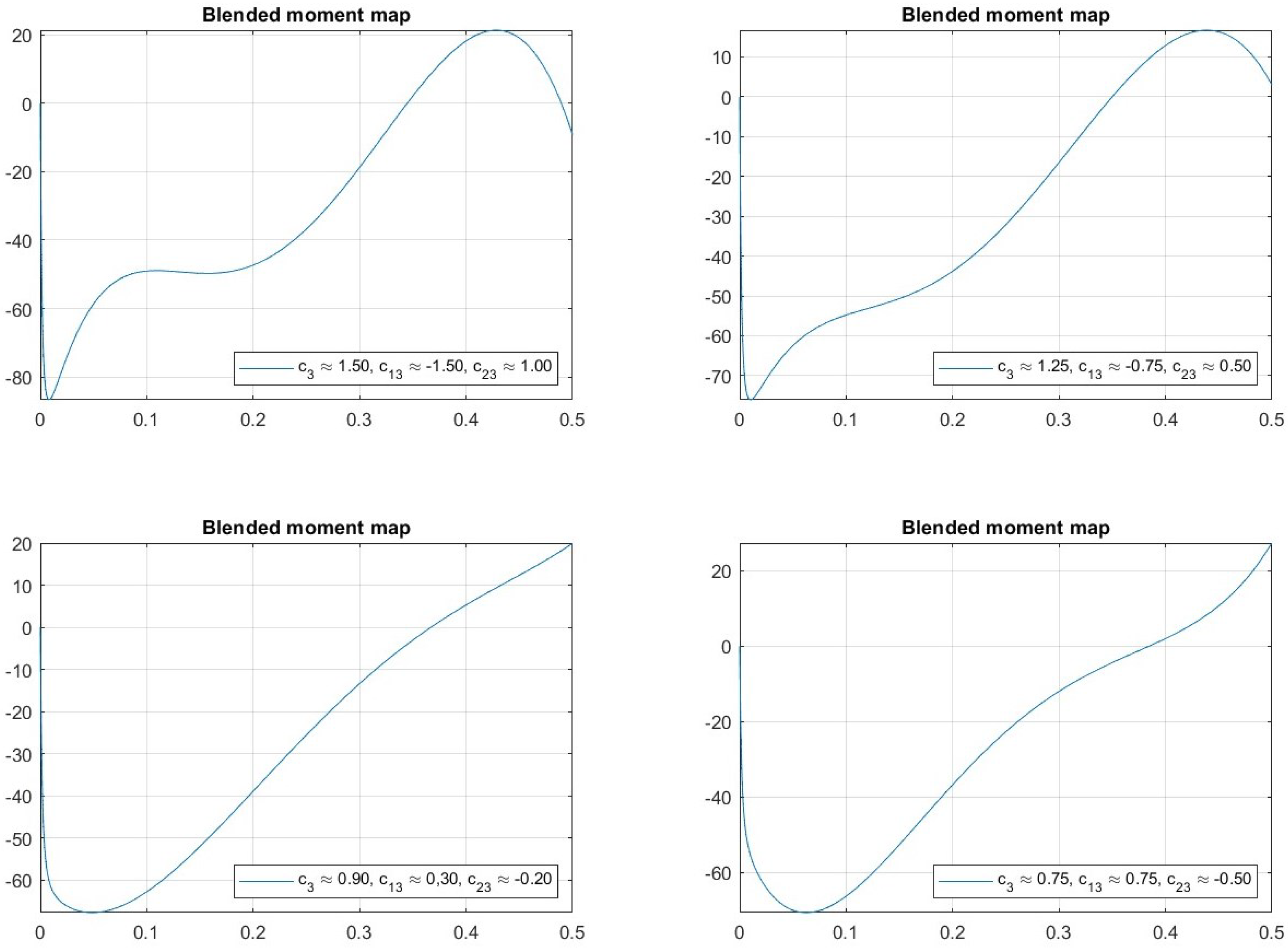
Trajectories with steeper ramps or stronger swinging-in or -out features can be modelled by different choices of the form parameters in the rational functions or in the polynomials of the higher order. In order to demonstrate the flexibility of the chosen method, in Figure 28, the results from other choices of the weights c 3 , c 13 , c 23 are illustrated:

5. Conclusions

In this study, we performed a comparison of various forward and backwards methods to deal with an overdetermined and originally analytically intractable ODE system. The resulting solution and moment functions, even though not computationally obtained by using a given external input, delivered results which were surprisingly good from a numerical perspective, compared to a benchmark formula close to the expected experimental reality reviewed earlier. For this reason, we are confident that in a more extended and systematic way of trying a greater variety of ansatz functions, this similarity could be improved almost arbitrarily.
In particular, the approximation of the ideal solution by Hermite splines of third and fifth order presented in Section 4.1 could almost certainly be further improved with Hermite splines of higher order; on the other hand, the abundance of the resulting appearing additional parameters is an issue which would certainly also have to be dealt with in a clever way. Since we already obtained surprisingly good results with the third- and fifth-order splines, we did not further evaluate these options.
In addition, as further approaches of the given type, we could imagine extending the principal ansatz (7) to more general types of the form
ϕ ( t ) = π 4 F g t τ
i.e., from the choice F ( x ) = x used in the present study to functions such as, e.g., F ( x ) = arctan ( x ) or other functions used as activation functions in neural networks.
We do not consider this study as a closed problem solution but rather as an initial step on a path which could lead to very fruitful alternative perspectives on ODE systems which initially are hard or impossible to tackle analytically. Of course, numerical solution methods are always possible and also valuable, but dealing with analytical formulas has the advantage of a much better intuitive understanding of the functions at hand.

Author Contributions

Both authors contributed equally to this article. All authors have read and agreed to the published version of the manuscript.

Funding

Open access funding was provided by the Zurich University of Applied Sciences (ZHAW).

Data Availability Statement

The data and code that support the findings of this study are available from the authors upon reasonable request.

Acknowledgments

We are grateful to our colleague Ruprecht Altenburger for helpful discussions.

Conflicts of Interest

On behalf of both authors, the corresponding author states that there are no conflicts of interest.

References

  1. Gajamohan, M.; Merz, M.; Thommen, I.; D’Andrea, R. The cubli: A cube that can jump up and balance. In Proceedings of the International Conference on Intelligent Robots and Systems, Vilamoura-Algarve, Portugal, 7–12 October 2012; pp. 3722–3727. [Google Scholar]
  2. Gajamohan, M.; Muehlebach, M.; Widmer, T.; D’Andrea, R. The cubli: A reaction wheel based 3d inverted pendulum. In Proceedings of the 2013 European Control Conference (ECC), Zurich, Switzerland, 17–19 July 2013; pp. 268–274. [Google Scholar]
  3. Muehlebach, M.; Mohanarajah, G.; D’Andrea, R. Nonlinear analysis and control of a reaction wheel-based 3d inverted pendulum. In Proceedings of the 52nd IEEE Conference on Decision and Control, Firenze, Italy, 10–13 December 2013; pp. 1283–1288. [Google Scholar]
  4. Muehlebach, M.; D’Andrea, R. Nonlinear analysis and control of a reaction- wheel-based 3-d inverted pendulum. IEEE Trans. Control Syst. Technol. 2017, 25, 235–246. [Google Scholar] [CrossRef]
  5. Lundberg, K.H.; Barton, T.W. History of inverted-pendulum systems. IFAC Proc. Vol. 2010, 42, 131–135. [Google Scholar] [CrossRef]
  6. Boubaker, O. The inverted pendulum: A fundamental benchmark in control theory and robotics. In Proceedings of the International Conference on Education and e-Learning Innovations, Sousse, Tunisia, 1–3 July 2012; pp. 1–6. [Google Scholar]
  7. Hofer, M.; Muehlebach, M.; D’Andrea, R. The one-wheel cubli: A 3d inverted pendulum that can balance with a single reaction wheel. Mechatronics 2023, 91, 102965. [Google Scholar] [CrossRef]
  8. Li, Z.; Yang, C.; Fan, L. (Eds.) Advanced Control of Wheeled Inverted Pendulum Systems, 1st ed.; Springer: London, UK, 2013. [Google Scholar]
  9. Boubaker, O.; Iriarte, R. (Eds.) The Inverted Pendulum in Control Theory and Robotics: From theory to new innovations. In Control, Robotics and Sensors; Institution of Engineering and Technology: Stevenage, UK, 2017. [Google Scholar]
  10. Altenburger, R.; Henrici, A.; Robbiani, M. Analytical solution of an ill-posed system of nonlinear ode’s. Commun. Nonlinear Sci. Numer. Simul. 2024, 130, 107762. [Google Scholar] [CrossRef]
  11. Smith, T. Mri artifacts and correction strategies. Imaging Med. 2010, 2, 445–457. [Google Scholar] [CrossRef]
  12. Xie, S.; Zheng, X.; Chen, Y.; Xie, L.; Liu, J.; Zhang, Y.; Yan, J.; Zhu, H.; Hu, Y. Artifact removal using improved googlenet for sparse-view ct reconstruction. Sci. Rep. 2018, 8, 6700. [Google Scholar] [CrossRef]
  13. Jiang, X.; Bian, G.-B.; Tian, Z. Removal of artifacts from eeg signals: A review. Sensors 2019, 19, 987. [Google Scholar] [CrossRef] [PubMed]
  14. Lee, S.S.; Lee, K.; Kang, G. Eeg artifact removal by bayesian deep learning & ica. In Proceedings of the 2020 42nd Annual International Conference of the IEEE Engineering in Medicine & Biology Society (EMBC), Montreal, QC, Canada, 20–24 July 2020; pp. 932–935. [Google Scholar]
  15. Nie, Y.; Guo, X.; Li, X.; Geng, X.; Quan, Z.; Zhu, G.; Yin, Z.; Zhang, J.; Wang, S. Real-time removal of stimulation artifacts in closed-loop deep brain stimulation. J. Neural Eng. 2021, 18. [Google Scholar] [CrossRef]
  16. Bertazzoli, G.; Esposito, R.; Mutanen, T.P.; Ferrari, C.; Ilmoniemi, R.J.; Miniussi, C.; Bortoletto, M. The impact of artifact removal approaches on tms–eeg signal. NeuroImage 2021, 239, 118272. [Google Scholar] [CrossRef]
  17. Ouyang, G.; Dien, J.; Lorenz, R. Handling eeg artifacts and searching individually optimal experimental parameter in real time: A system development and demonstration. J. Neural Eng. 2022, 19, 016016. [Google Scholar] [CrossRef]
  18. Chen, P.; Kim, T.; Rijn, E.D.; Provenza, N.R.; Sheth, S.A.; Goodman, W.K.; Borton, D.A.; Harrison, M.T.; Darbon, J. Periodic artifact removal with applications to deep brain stimulation. IEEE Trans. Neural Syst. Rehabil. Eng. 2022, 30, 2692–2699. [Google Scholar] [CrossRef] [PubMed]
  19. Bahador, N.; Saha, J.; Rezaei, M.R.; Utpal, S.; Ghahremani, A.; Chen, R.; Lankarany, M. Robust removal of slow artifactual dynamics induced by deep brain stimulation in local field potential recordings using svd-based adaptive filtering. Bioengineering 2023, 10, 719. [Google Scholar] [CrossRef]
  20. Wang, F.; Chen, X.; Roelfsema, P.R. Comparison of electrical microstimulation artifact removal methods for high-channel-count prostheses. J. Neurosci. Methods 2024, 408, 110169. [Google Scholar] [CrossRef] [PubMed]
  21. Chuang, C.-H.; Chang, K.-Y.; Huang, C.-S.; Bessas, A.-M. Art: Artifact removal transformer for reconstructing noise-free multichannel electroencephalographic signals. arXiv 2024, arXiv:2409.07326. [Google Scholar]
  22. Gransier, R.; Carlyon, R.; Richardson, M.; Middlebrooks, J.; Wouters, J. Artifact removal by template subtraction enables recordings of the frequency following response in cochlear-implant users. Sci. Rep. 2024, 14, 6158. [Google Scholar] [CrossRef]
  23. Yan, P.; Abdulkadir, A.; Luley, P.-P.; Rosenthal, M.; Schatte, G.A.; Grewe, B.F.; Stadelmann, T. A comprehensive survey of deep transfer learning for anomaly detection in industrial time series: Methods, applications, and directions. IEEE Access 2024, 12, 3768–3789. [Google Scholar] [CrossRef]
  24. Darban, Z.Z.; Webb, G.I.; Pan, S.; Aggarwal, C.; Salehi, M. Deep learning for time series anomaly detection: A survey. ACM Comput. Surv. 2024, 57, 1–42. [Google Scholar] [CrossRef]
  25. Kassel, G. A formal ontology of artefacts. Appl. Ontol. 2010, 5, 223–246. [Google Scholar] [CrossRef]
  26. Keaveny, T.M.; Borchers, R.E.; Gibson, L.J.; Hayes, W.C. Theoretical analysis of the experimental artifact in trabecular bone compressive modulus. J. Biomech. 1993, 26, 599–607. [Google Scholar] [CrossRef]
  27. Nakano, T.; Nakashima, Y. Analytical expressions for the reconstructed image of a homogeneous cylindrical sample exhibiting a beam hardening artifact in x-ray computed tomography. J. X-Ray Sci. Technol. 2018, 26, 1–15. [Google Scholar] [CrossRef]
  28. Miller, M.S.; Straight, C.R.; Palmer, B.M. Inertial artifact in viscoelastic measurements of striated muscle: Modeling and experimental results. Biophys. J. 2022, 121, 1424–1434. [Google Scholar] [CrossRef] [PubMed]
  29. Kumar, D.; Kaplan, M.; Haque, M.R.; Osman, M.S.; Baleanu, D. A variety of novel exact solutions for different models with the conformable derivative in shallow water. Front. Phys. 2020, 8, 177. [Google Scholar] [CrossRef]
  30. Fadhal, E.; Akbulut, A.; Kaplan, M.; Awadalla, M.; Abuasbeh, K. Extraction of exact solutions of higher order sasa-satsuma equation in the sense of beta derivative. Symmetry 2022, 14, 2390. [Google Scholar] [CrossRef]
  31. Wang, X.; Javed, S.A.; Majeed, A.; Kamran, M.; Abbas, M. Investigation of exact solutions of nonlinear evolution equations using unified method. Mathematics 2022, 10, 2996. [Google Scholar] [CrossRef]
  32. Neto, J.G.M.N.; Fonseca, E.J.; Jesus-Silva, A.J. Exact solutions for non-rayleigh nondiffracting speckles. Phys. Rev. A 2022, 106, 053519. [Google Scholar] [CrossRef]
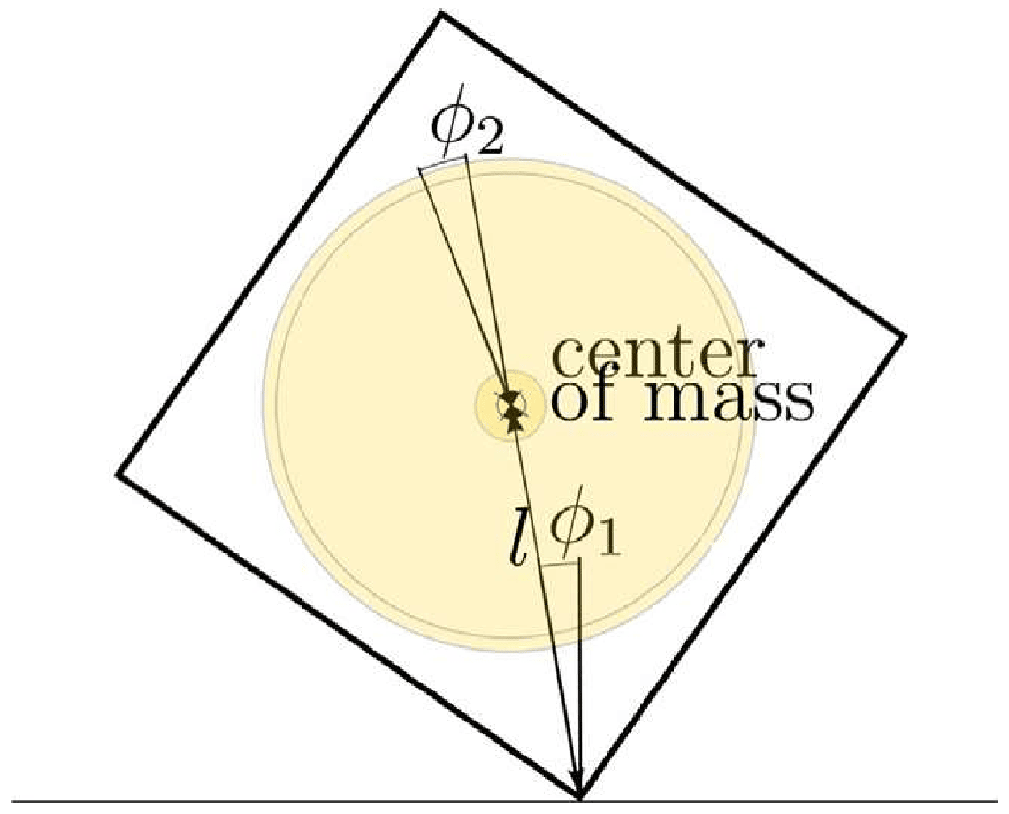
Figure 1. Cubli.
Figure 1. Cubli.
Mathematics 12 03675 g001
Figure 2. Cubli in motion.
Mathematics 12 03675 g002
Figure 3. Analytical model of experimental artefacts.
Mathematics 12 03675 g003
Figure 4. Ideal angle trajectory.
Mathematics 12 03675 g004
Figure 5. Ideal moment trajectory.
Mathematics 12 03675 g005
Figure 6. Switch-on ramp.
Mathematics 12 03675 g006
Figure 7. Final swing-in.
Mathematics 12 03675 g007
Figure 8. Angle functions.
Mathematics 12 03675 g008
Figure 9. Moment functions.
Mathematics 12 03675 g009
Figure 10. Angle trajectories.
Mathematics 12 03675 g010
Figure 11. Comparison of deviations from forward solution.
Mathematics 12 03675 g011
Figure 12. Moment trajectories.
Mathematics 12 03675 g012
Figure 13. Comparison of deviations from forward solution.
Mathematics 12 03675 g013
Figure 14. Angle trajectories.
Mathematics 12 03675 g014
Figure 15. Moment trajectories.
Mathematics 12 03675 g015
Figure 16. Angle trajectories.
Mathematics 12 03675 g016
Figure 17. Moment trajectories.
Mathematics 12 03675 g017
Figure 18. Angle trajectories.
Mathematics 12 03675 g018
Figure 19. Moment trajectories.
Mathematics 12 03675 g019
Figure 20. Angle trajectories.
Mathematics 12 03675 g020
Figure 21. Moment trajectories.
Mathematics 12 03675 g021
Figure 22. Angle trajectories.
Mathematics 12 03675 g022
Figure 23. Moment trajectories.
Mathematics 12 03675 g023
Figure 24. Dependence on first parameter.
Mathematics 12 03675 g024
Figure 25. Dependence on second form parameter.
Mathematics 12 03675 g025
Figure 26. Angle trajectories.
Mathematics 12 03675 g026
Figure 27. Moment trajectories.
Mathematics 12 03675 g027
Figure 28. Trajectories from other choices of the form parameters.
Mathematics 12 03675 g028
Disclaimer/Publisher’s Note: The statements, opinions and data contained in all publications are solely those of the individual author(s) and contributor(s) and not of MDPI and/or the editor(s). MDPI and/or the editor(s) disclaim responsibility for any injury to people or property resulting from any ideas, methods, instructions or products referred to in the content.