Article

Anomaly Detection Based on Graph Convolutional Network–Variational Autoencoder Model Using Time-Series Vibration and Current Data

1
Advanced Mechatronics Research Group, Daegyeong Division, Korea Institute of Industrial Technology, Daegu 42994, Republic of Korea
2
Department of Electronics Engineering, Pusan National University, Busan 46241, Republic of Korea
*
Author to whom correspondence should be addressed.
Mathematics 2024, 12(23), 3750; https://doi.org/10.3390/math12233750
Submission received: 18 October 2024 / Revised: 25 November 2024 / Accepted: 27 November 2024 / Published: 28 November 2024
(This article belongs to the Section E2: Control Theory and Mechanics)

Abstract

:
This paper proposes a deep learning-based anomaly detection method using time-series vibration and current data, which were obtained from endurance tests on driving modules applied in industrial robots and machine systems. Unlike traditional classification models that depend on labeled fault data for detection, acquiring sufficient fault data in real industrial environments is highly challenging due to various conditions and constraints. To address this issue, we employ a semi-supervised learning approach that relies solely on normal data to effectively detect abnormal patterns, overcoming the limitations of conventional methods. The performance of semi-supervised models was first validated using a statistical feature-based anomaly detection approach, from which the GCN-VAE model was adopted. By combining the spatial feature extraction capability of Graph Convolutional Networks (GCNs) with the latent temporal feature modeling of Variational Autoencoders (VAEs), our method can effectively detect abnormal signs in the data, particularly in the lead-up to system failures. The experimental results confirmed that the proposed GCN-VAE model outperformed existing hybrid deep learning models in terms of anomaly detection performance in the pre-failure section.

1. Introduction

Artificial intelligence (AI) and machine learning technologies have significantly enhanced the efficiency, stability, and accuracy of robotic and mechanical systems. These advancements have played a crucial role in accelerating production automation across diverse industries, further elevating the importance of robots in complex manufacturing processes. However, maintaining the continuous stability and reliability of these systems remains a significant challenge [1,2,3,4].
In industrial environments, early diagnosis and prevention of faults in robotic systems are essential yet highly challenging tasks. Traditional fault diagnosis methods typically rely on data collected from both normal and faulty states to classify fault occurrences. While effective for monitoring conditions, these methods face several limitations [5,6,7,8]:
  • Lack of fault data: Collecting normal data is relatively straightforward in industrial environments, but obtaining fault data is significantly more difficult. Robots typically halt operation upon experiencing a fault, preventing data collection at the moment of failure. Furthermore, faults are infrequent and unpredictable, making it challenging to gather sufficient fault data.
  • Diversity of data features: Mechanical characteristics of robots result in differences between initial-state data and data collected over time as the system’s durability decreases. Consequently, even for the same robot, data features can change over time, complicating fault detection using a classification model.
  • Variability of environmental and operating conditions: Data features for robots with identical specifications can vary significantly depending on environmental factors and operating conditions. This variability leads to differences in fault timing and types, making consistent detection of pre-failure signals across diverse conditions highly challenging.
To address these challenges, anomaly detection has emerged as a promising alternative. Unlike traditional fault diagnosis methods, anomaly detection identifies deviations from normal data patterns, making it particularly useful in environments with limited fault data [9,10,11,12]. In particular, semi-supervised anomaly detection is effective at capturing subtle pre-failure anomalies by relying solely on normal data. Furthermore, this approach eliminates the dependence on labeled fault data, enabling robust anomaly detection in dynamic and unpredictable industrial environments [13,14].
This paper proposes a semi-supervised Graph Convolutional Network (GCN)–Variational Autoencoder (VAE) model for detecting anomalies in time-series vibration and current data collected from durability tests on driving modules. The key contributions of this study are as follows:
  • Integration of vibration and current data: This study enhances anomaly detection performance by integrating vibration and current data, leveraging the complementary features of these two types of data. This approach effectively detects subtle anomaly signals that deviate from normal patterns, addressing the limitations of single-sensor-based methods while providing a more comprehensive understanding of anomalies.
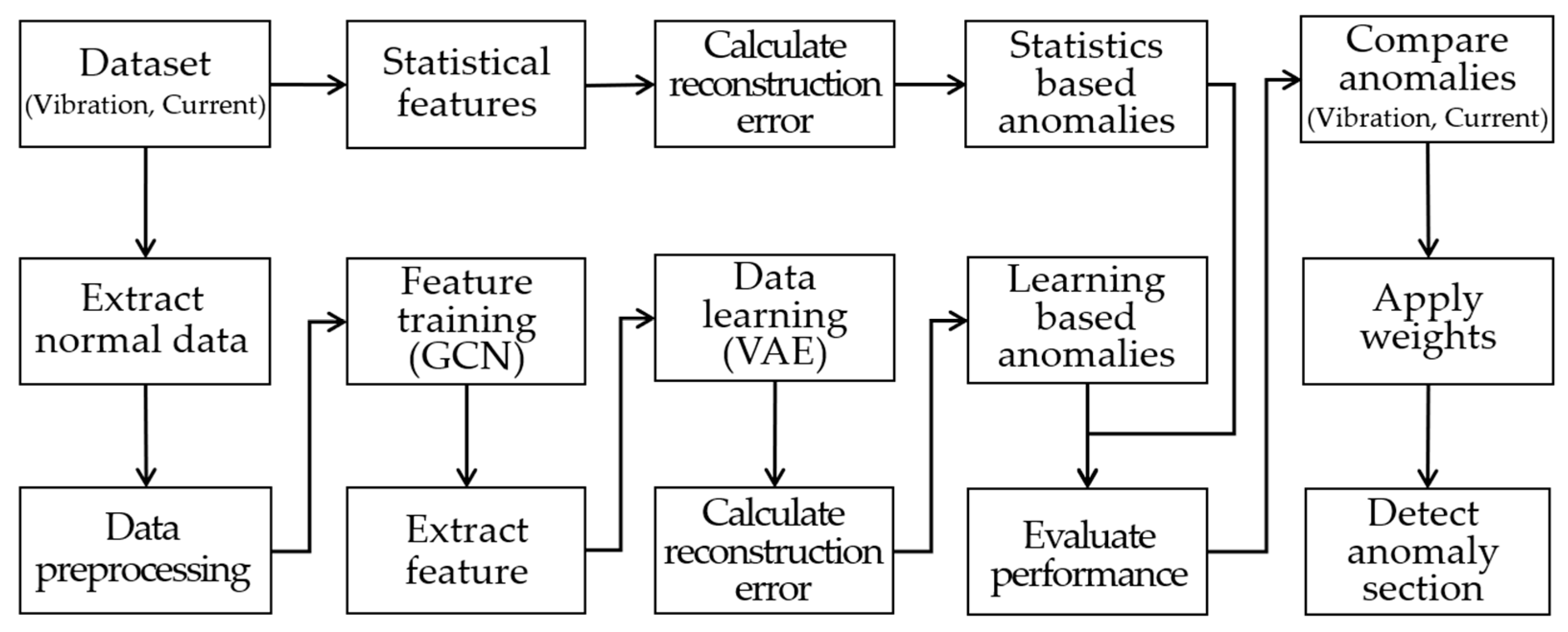
  • Validation using statistical feature-based anomaly detection: This study introduces a novel comparison framework to validate the anomaly detection performance of deep learning models against statistical feature-based methods. Statistical feature-based anomaly detection utilizes the entire dataset to detect anomalies through filtering, RMS variation rates, and reconstruction errors, whereas the deep learning models rely solely on the initial data for anomaly detection. By leveraging this statistical baseline, this study evaluates the performance of individual deep learning models and assesses the suitability of hybrid deep learning models.
  • Semi-supervised learning with GCN-VAE: To effectively detect pre-failure anomaly signals, a novel semi-supervised learning-based GCN-VAE model is proposed. The model extracts spatial features by incorporating temporal continuity and inter-data relationships, mapping these features into a latent space to identify abnormal patterns effectively through reconstruction errors.
  • Weighted anomaly detection considering temporal progression and continuity: To enhance the detection performance of pre-failure anomalies, this study introduces a weighting mechanism that accounts for both temporal progression and the continuity of detected anomalies. This mechanism increases the detection probability for subtle anomaly signals that evolve over time and emphasizes the significance of consecutive anomalies, enabling more effective detection of pre-failure anomalies. By integrating this weighting mechanism, the GCN-VAE model demonstrated exceptional anomaly detection performance, even in scenarios characterized by high noise levels and complex temporal dependencies.
The remainder of this paper is organized as follows: Section 2 reviews related work, while Section 3 describes the conditions and methods of the durability tests for driving modules. Section 4 presents experimental comparisons between the anomaly detection performance of existing hybrid deep learning models and the proposed model, confirming its effectiveness. Finally, Section 5 concludes this study and suggests directions for future research.

2. Related Works

Anomaly detection plays a critical role in early fault diagnosis of robotic systems, with semi-supervised learning techniques gaining significant attention. These techniques rely exclusively on normal data for training, identifying deviations from normal patterns as anomalies. This makes them particularly valuable in scenarios where fault data are unavailable or highly imbalanced [15,16].
Commonly used semi-supervised anomaly detection methods include Anomaly Detection with Generative Adversarial Networks (AnoGAN), Long Short-Term Memory (LSTM), VAE, Transformer, and GCN. These deep learning models have been successfully applied across various industrial domains [17,18,19].
Recently, hybrid deep learning models have been proposed to achieve superior anomaly detection performance by combining the strengths of multiple models. For instance, Fan et al. (2023) utilized a Temporal Convolutional VAE-GAN model to achieve high sensitivity in detecting early weak faults in bearings using wind turbine datasets [20]. Ou et al. (2021) introduced a Deep Sequence Multi-Distribution Adversarial (DSMDA) model, combining an LSTM-based Variational Autoencoder (VAE) with a dual-discriminator GAN framework, achieving both high sensitivity and robustness compared to existing methods [21]. Yang et al. (2023) proposed a Deep Capsule Graph Convolutional Network (DCGCN) to diagnose compound faults in harmonic drives, demonstrating strong performance under varying working conditions [22]. Yan et al. (2024) proposed Unsuper-TDGCN, an unsupervised model combining Transformer and Dynamic Graph Convolutional Network (DyGCN) for machine anomalous sound detection under domain shifts, achieving superior performance across diverse datasets [23].
Among these methods, GCN has proven highly effective in modeling spatial and relational data by leveraging graph structures to capture interdependencies between data points. This makes it particularly valuable for anomaly detection in structured datasets [24]. Similarly, VAE excels in learning normal patterns and detecting deviations through reconstruction errors, enabling it to identify subtle anomalies that are often overlooked by traditional methods. This capability is especially beneficial in scenarios with limited or imbalanced fault data [25].
Despite their strengths, GCN and VAE have inherent limitations. While GCN specializes in capturing spatial and relational features, it lacks a mechanism to model temporal dependencies or detect subtle anomaly signals. Conversely, VAE’s reconstruction-based approach effectively identifies temporal deviations but does not account for spatial relationships. These complementary strengths and limitations underscore the need for an integrated approach.
To overcome these limitations, this study proposes a semi-supervised GCN-VAE model for detecting anomalies in time-series vibration and current data collected from durability tests on driving modules. The proposed model explicitly integrates temporal continuity and inter-data relationships into a unified framework, effectively bridging the gap between spatial and temporal analysis to maximize performance. Consequently, the GCN-VAE model demonstrates exceptional capability in identifying subtle pre-failure anomalies, particularly in complex and noisy industrial environments.

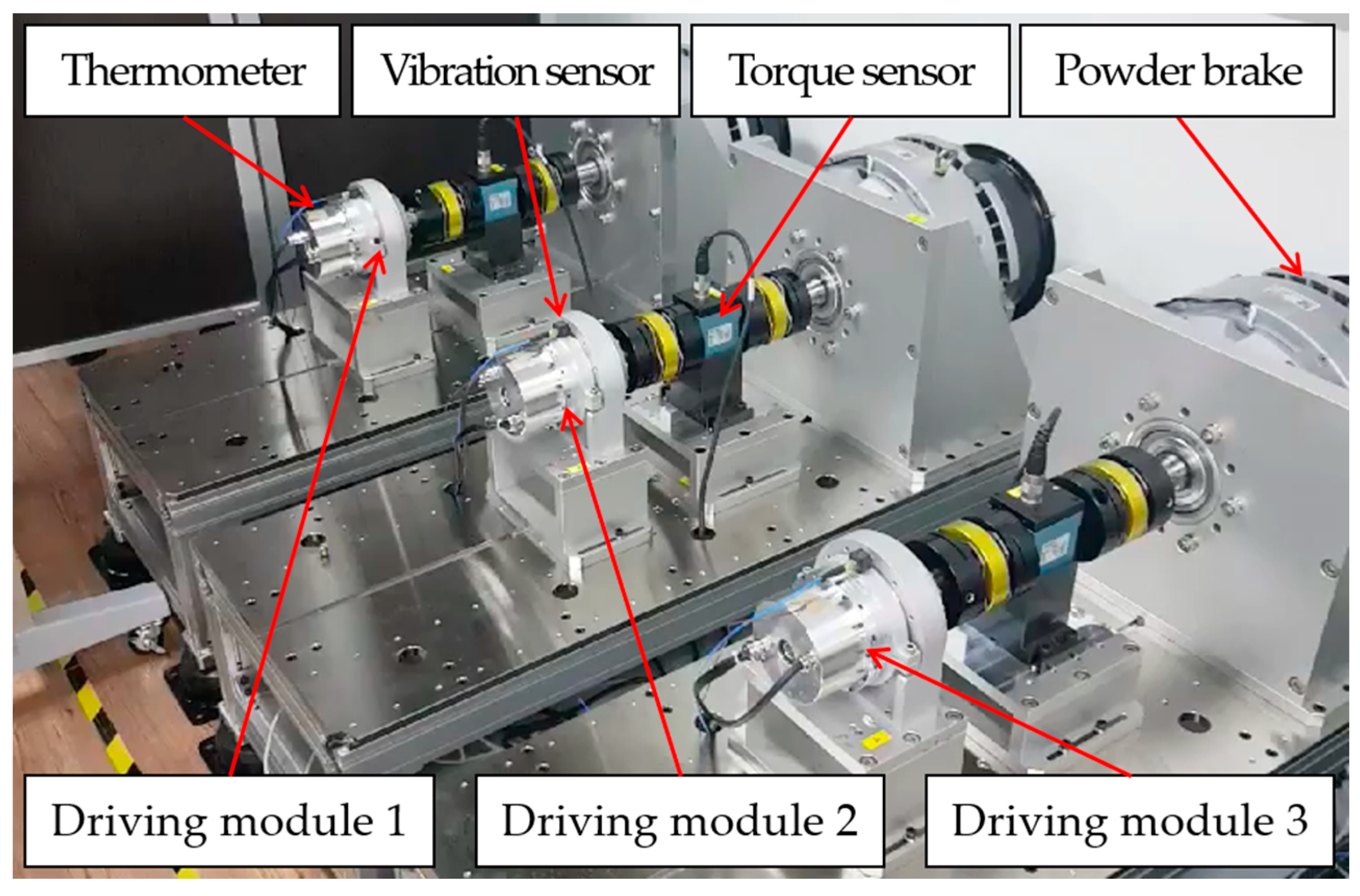
3. Conditions and Methods of Endurance Test for the Driving Modules

In this study, we conducted endurance tests using commercial driving modules applied to robots and mechanical systems in an industrial site, and time series vibration and current-related data were collected during the process. The endurance test environment can be found in Figure 1.
The driving module used in this test was KaiserDrive KAH-25EL 5BE (rated power 500 W, maximum average torque 133 Nm, rated speed 16.2 RPM), manufactured by KaiserDrive, located in Suzhou, China. The vibration sensor used was a PCB 356A17 (three-axis accelerometer; sensitivity of 500 mV/g; measurement range of ±98 m/s2 pk; frequency range of 0.4–4000 Hz), manufactured by PCB Piezotronics, located in Depew, NY, USA.
Figure 2 shows the position, velocity, and torque values of the driving modules in line with the condition of the endurance test. After applying torque to the three modules according to the test conditions in the environment presented in Table 1, we continuously performed forward and reverse rotations. We collected data for 20 s every 10 min in a 1 kHz sampling cycle. In this study, we only utilized data in the constant velocity section by considering the stability of the data, and the 10 min data cycle was defined as one cycle for the anomaly detection experiment.
Figure 3 displays the raw data and root mean square (RMS) values of vibration and current signal data obtained from the endurance tests of the driving modules. Module 1 operated 10,885 cycles (approximately 1814 h), Module 2 operated 3117 cycles (around 519 h), and Module 3 operated 5292 cycles (about 882 h), and then faults occurred.

4. Anomaly Detection Test Results of the Driving Modules

We utilized datasets obtained from the endurance tests of commercial driving modules to establish anomaly detection methods for robot systems. In Section 4.1, we conducted anomaly detection experiments based on statistical features using the entire dataset. In Section 4.2, we performed anomaly detection experiments by applying various deep learning models to only a portion of the normal data and comparing their performance.

4.1. Anomaly Detection Based on Statistical Features

In statistical feature-based anomaly detection, we selected the Savitzky–Golay filter to reduce noise and spikes in time-series data while preserving the essential shape and peaks of the original signal. While other filtering methods, such as spline smoothing, Fourier transform, Gaussian kernel filtering, and discrete wavelet transform, have been proposed for peak processing, many encounter computational challenges when handling highly corrupted signals. In contrast, the Savitzky–Golay filter performs a local polynomial regression on the data within a moving window, enabling it to smooth the data while retaining high-frequency components and sharp signal features [26,27]. This characteristic makes it particularly suitable for vibration data, where preserving peak amplitudes and waveform shapes is crucial for anomaly detection.
A limitation of the Savitzky–Golay filter is that it can cause edge distortions when surrounding data points are insufficient. To address this, we adjusted the filter’s window size and polynomial order and applied data padding to minimize boundary distortion. To achieve smooth filtering while preserving the high-frequency components of the data, we set the filter’s window size to 11 and the polynomial order to 2. These parameters were experimentally selected and optimized to maintain the primary features of the vibration signal without excessive smoothing. The equation below provides the formula for the Savitzky–Golay filter.
y i = j = m m c j · x i + j ;
where y i is the filtered signal; x i + j is the original signal; c j is the polynomial coefficient; and m is the window size of the filter. This filter plays a crucial role in reducing noise while maintaining local patterns in the data.
To detect anomalies in the time series data, we combined the reconstruction error and change rate of RMS and selected the final anomalies. First, regarding the reconstruction error, the difference between each data point was calculated based on the statistical distribution of the normal data. Then, a threshold was set to separate the anomalies [28,29,30]. The reconstruction error can be calculated as follows:
E r e c o n s t r u c t i o n = i = 1 n x i x ^ i 2 ;
where x i and x ^ i are the original and the reconstructed data, respectively. This error allows us to numerically evaluate the difference between the data.
Furthermore, the change rate of RMS can be calculated using the first derivative of the signal to detect the section where the vibration data changes rapidly. The change rate of RMS can be calculated as follows:
C h a n g e   r a t e   o f   R M S = d d t 1 n i = 1 n x i 2 ;
where d x i d t is the first derivative value of the signal. The section where the change rate of RMS exceeds a certain threshold was selected as an anomaly section.
Figure 4 presents the results of anomaly detection using a statistical feature-based method. First, the reconstruction error was calculated as the difference between the filtered signal and the reconstructed data, with any error exceeding the threshold considered an anomaly. The RMS rate of change was determined using the first derivative of the signal to detect regions of abrupt variation, identifying segments that exceeded the set threshold as anomalies. Based on experimental analysis, this study selected a threshold of 0.98 for reconstruction error and 0.57 for the RMS rate of change.
The detection results indicate that in Module 1, anomalies were detected in both the vibration and current data towards the latter part of the dataset, just before failure. In Module 2, anomalies were observed in the vibration data in certain early segments, with clear anomalies detected in both vibration and current data right before the failure. In Module 3, multiple anomalies were detected in both vibration and current data during the middle section and just before failure. These anomaly detection results based on statistical features were performed on the entire dataset and used as baseline values for evaluating the performance of the deep learning model in this study.

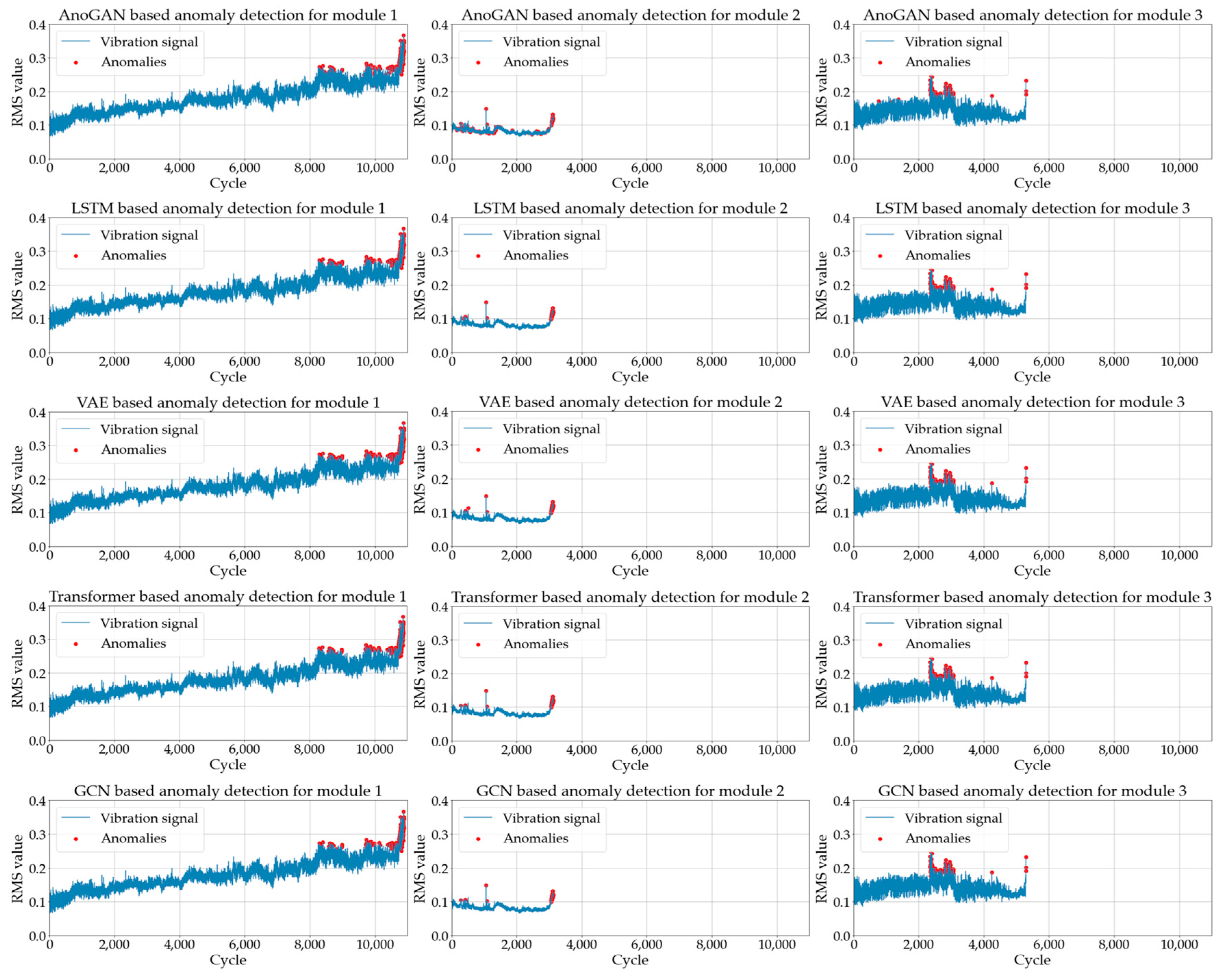
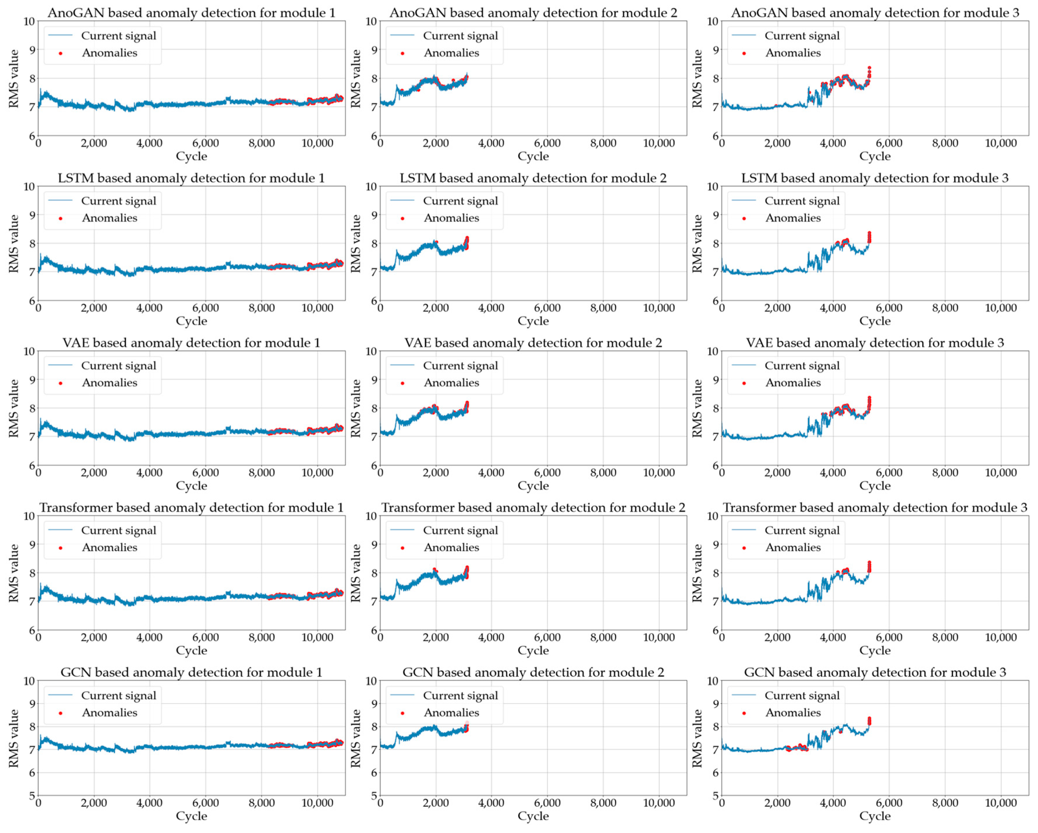
4.2. Anomaly Detection Based on a Deep Learning Model

To compare the performance of deep learning-based anomaly detection models, normal data obtained from driving modules was applied to semi-supervised learning models, including AnoGAN, LSTM, VAE, Transformer, and GCN. Normal data for vibration and current were extracted from the first 100 data cycles of each module and used for model training. The training and testing configurations were as follows: (1) Modules 1 and 2 were used for training, with Module 3 designated for testing; (2) Modules 1 and 3 were used for training, with Module 2 designated for testing; and (3) Modules 2 and 3 were used for training, with Module 1 designated for testing.
Figure 5 and Figure 6 show the results of anomaly detection after applying normal vibration and current data to each deep learning model. In Module 1, anomalies were detected in the later part of the data and the pre-failure section. In Module 2, anomalies were detected in the earlier part of the data and the pre-failure section, while in Module 3, anomalies were detected in the middle part of the data and the pre-failure section.
The visual comparison of the statistical feature-based anomaly detection results in Figure 4 with the deep learning-based results in Figure 5 and Figure 6 reveals the following insights. AnoGAN exhibited a tendency to detect excessive anomalies across all modules for both vibration and current signals compared to the statistical feature-based method. The LSTM, VAE, and Transformer models demonstrated anomaly detection results that were nearly identical to the statistical feature-based method for vibration signals. However, for current signals, Modules 2 and 3 showed slight discrepancies in the middle and later parts of the data. In contrast, the GCN model produced anomaly detection results that were almost entirely consistent with the statistical feature-based method across all modules for both vibration and current signals. Notably, the GCN model exhibited an exceptional anomaly detection performance in the pre-failure section, further emphasizing its effectiveness and reliability.
Table 2 presents a comparison of anomaly detection matching accuracy between statistical feature-based methods and deep learning models. Among the deep learning models, GCN achieved the highest matching accuracy, followed by Transformer, VAE, LSTM, and AnoGAN. For vibration signals, LSTM, VAE, Transformer, and GCN models showed excellent performance, achieving over 99% matching accuracy with the statistical feature-based results. However, for current signals, the detection accuracy of Transformer, VAE, LSTM, and AnoGAN models was relatively lower. In contrast, the GCN model demonstrated outstanding performance, maintaining over 99% anomaly detection accuracy even for current signals.
The statistical feature-based anomaly detection method serves as a useful benchmark for evaluating the performance of deep learning models but faces challenges in achieving high accuracy for detecting pre-failure anomalies. To address this limitation, this study proposes the GCN-VAE model, which integrates GCN’s ability to capture structural relationships among data points with VAE’s reconstruction-based anomaly detection approach. While VAE focuses on representing individual data points in a latent space, GCN complements this by modeling spatial and temporal dependencies, enabling the effective detection of subtle anomaly signals that might otherwise be overlooked by traditional methods.
The final algorithm of the GCN-VAE-based anomaly detection proposed in this study can be found in Figure 7. After extracting normal data from the time series of vibration and current data obtained through endurance tests of the driving modules, a preprocessing process occurs before being applied to the model. In this preprocessing phase, anomaly peaks are removed, and the data are refined by adjusting the arrangement of the data so that features can be extracted well. The preprocessed data are divided into statistical feature-based anomaly detection and GCN-VAE learning model-based anomaly detection. In statistical feature-based anomaly detection, the Savitzky–Golay filter is applied to remove noise in the data. Then, the reconstruction error is calculated based on statistical features and combined with the change rate of RMS to detect data outside the range of normal data as anomalies. At the same time, in the GCN-VAE learning model-based anomaly detection, GCN is employed to extract the spatial features of the input data. The feature vector between each node is calculated and delivered to the VAE’s encoder. VAE maps the input data into the latent space and then is restored again to the original data. The reconstruction error calculated in this process determines whether the data exist within the normal range and detects data exceeding the threshold as anomalies. The anomaly detection process is performed independently by the statistical feature-based method and the GCN-VAE-based method, respectively, and the anomalies detected by both methods are compared. Then, the detected results of these two methods are compared, model performances are evaluated, and the accuracy of detected anomalies is confirmed. Finally, based on the performance evaluations, detected vibration and current anomalies are compared for each cycle, weights are applied, and the final anomaly section is detected.
The GCN model is designed to process graph-structured data by leveraging node and edge information to extract spatial and relational features. In this study, each node represents an individual cycle of time-series vibration and current data obtained from durability tests on driving modules. These features are directly derived from raw time-series data, allowing the model to learn intrinsic spatial and temporal patterns without relying on pre-computed statistical metrics. Temporal relationships between cycles are encoded as edges, determined by the sequential order of the data. Uniform edge weights are assigned to represent the temporal progression, preserving the natural dependencies within the dataset. The graph-based structure allows GCN to model temporal dependencies essential for early failure detection [31,32].
Unlike traditional machine learning models, which treat data points as independent entities, GCNs utilize graph convolution operations to aggregate information from neigh-boring nodes. This process transforms raw input features into higher-dimensional embeddings that encapsulate both local and global patterns across the graph. By analyzing these embeddings, the GCN can identify subtle pre-failure anomalies more effectively.
The layer structure of the GCN is designed to learn by combining node information with that of adjacent nodes. Each layer H l + 1 is updated based on the node features H l from the previous layer and the adjacency matrix A ~ , as shown in the following equation [33].
H l + 1 = σ D ~ 1 / 2 A ~ D ~ 1 / 2 H l W l ;
where H ( l ) is the feature of the node in the l th layer; σ is the activation function; A ~ is the adjacency matrix with added self-connections; D ~ is the normalized diagonal matrix; and W l is the learned weight.
The GCN processes the input data x and the edge index of the graph through multiple layers to extract feature vectors for each node. These feature vectors, representing the spatial and relational characteristics of the graph-structured data, are subsequently passed to the encoder of the VAE. The VAE leverages these feature vectors to learn a latent space representation, denoted as z. During training, the VAE maps the input data into the latent space via its encoder and reconstructs the data through its decoder, enabling the identification of anomalies by capturing deviations from normal patterns [34]. The loss function of L x of VAE consists of the reconstruction loss and KL divergence is expressed as follows:
L x = E q ( z | x ) log p ( x | z ) + D K L q ( z | x ) p ( z ) ;
where x is the input data; z is the latent variable; E is the expected value of the distribution of the latent variable z ; p ( x | z ) is the likelihood distribution of x predicted by the decoder; q ( z | x ) is the posterior probability distribution of the latent variable z estimated by the encoder; p ( z ) is the prior distribution of the latent space z ; and D K L is the KL divergence, which measures the difference between the two probability distributions.
During the learning process, GCN employs mean squared error (MSE) loss to minimize the difference between the input and output features, training the feature vector of each node. The output feature vector from GCN is fed into the VAE encoder to generate the latent space vector z , which is then used by the decoder to reconstruct the original data. The VAE’s learning process utilizes reconstruction loss and KL divergence, as outlined in Equation (5).
The final loss function is calculated as a weighted sum of the losses of GCN and VAE. The loss of GCN is based on the difference between the input data and the extracted node feature vector. The loss of VAE reflects the difference between the original and restored data and the latent spatial distribution. In this process, GCN and VAE are trained using separate optimizers. After the training is complete, the reconstruction error is calculated for each node, and if this error exceeds a set threshold, the node is detected as an anomaly (Algorithm 1).
Algorithm 1 GCN-VAE Based Anomaly Detection
Require: train and test dataset D t r a i n , D t e s t
01: Initialize: GCN model G G C N , VAE model G V A E , optimizer O G C N , O V A E
02: Define Loss function L = L G C N + β L V A E
03: Construct graph G ( V ,   E ) from D t r a i n
04: For each epoch e = 1   t o   N :
05:    For each mini-batch X b ,   E b from G
06:       Compute GCN output h G C N = G G C N X b ,   E b
07:       Compute  L G C N = M S E h G C N , X b
08:       Update GCN weights using O G C N and L G C N
09:    end for
10:    For each mini-batch X b ,   E b from G :
11:       Encode GCN output into latent space: z = G V A E _ e n c ( h G C N )
12:       Reconstruct data from latent space: X ^ = G V A E _ d e c ( z )
13:       Compute VAE reconstruction loss L V A E = M S E X ^ , X b + K L
14:       Update VAE weights using O V A E and L V A E
15:    end for
16:    Compute overall loss L = L G C N + β L V A E
17: end for
18: Anomaly detection on D t e s t :
19: For each node v V :
20:    Compute reconstruction error E v = X v X ^ v 2 2
21: end for
22: Return: Anomalies detected where E v > t h r e s h o l d
The vibration and current anomalies detected by the GCN-VAE model are compared at each cycle and weighted to calculate the final anomaly probability. An anomaly section is selected based on this. Equation (6) indicates the weight used to detect the final anomaly section. The weights increase over time, and the more consecutive anomalies occur, the larger the value assigned becomes. In other words, the weight over time is multiplied by the weight for the continuity of the anomaly to determine the final anomaly section [35,36,37].
W t , n = log 1 + α t × β n ;
where t is the value of the current time (cycle); α is the weight control constant; n is the number of consecutive anomalies; and β is a weight control constant in line with the continuity of the anomalies.
Figure 8 provides a visual comparison of the anomaly detection results for normal vibration and current data from the driving module, as applied to the VAE-GAN, LSTM-VAE, GCN-Transformer, and the proposed GCN-VAE models. In Module 1, all models successfully detected anomalies in the pre-failure section. However, the VAE-GAN, LSTM-VAE, and GCN-Transformer models tended to show high anomaly probabilities not only in the pre-failure section but also in the later part of the data. In contrast, the proposed GCN-VAE model exhibited relatively fewer anomaly segments and lower anomaly probabilities in the later part, while achieving a higher anomaly probability than the other models in the pre-failure section, demonstrating more effective anomaly detection. In Module 2, all models recorded high anomaly probabilities only in the pre-failure section, showing excellent detection performance. In Module 3, all models showed somewhat lower anomaly probabilities in the middle and later parts but demonstrated strong anomaly detection performance in the pre-failure section. Notably, the proposed GCN-VAE model exhibited significantly higher anomaly detection performance in the pre-failure section compared to the other models.
Table 3 shows the comparison of anomaly scores calculated for the pre-failure section in each hybrid deep learning model based on the experiment in Figure 8. The anomaly detection performance of each model was scored according to the number of cycles before failure. The formula for the anomaly score is as follows:
A n o m a l y   s c o r e = 1 M i = N M + 1 N P i ;  
where N is the total number of cycles; M is the number of cycles in the section just before the failure; and P ( i ) is the anomaly probability for the cycle i . P ( i ) is the weighted anomaly probability calculated in Equation (6).
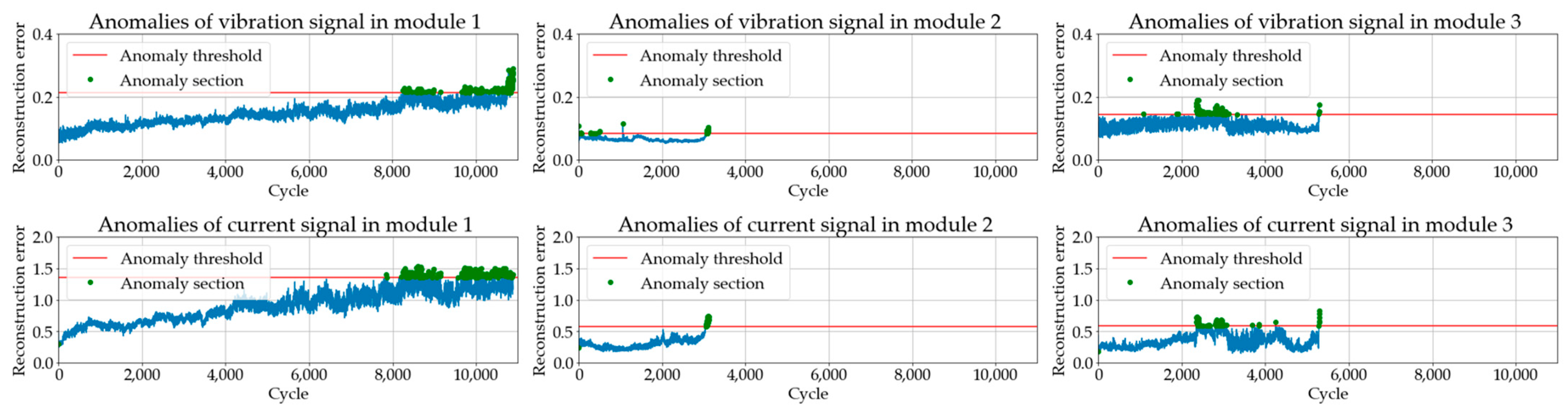
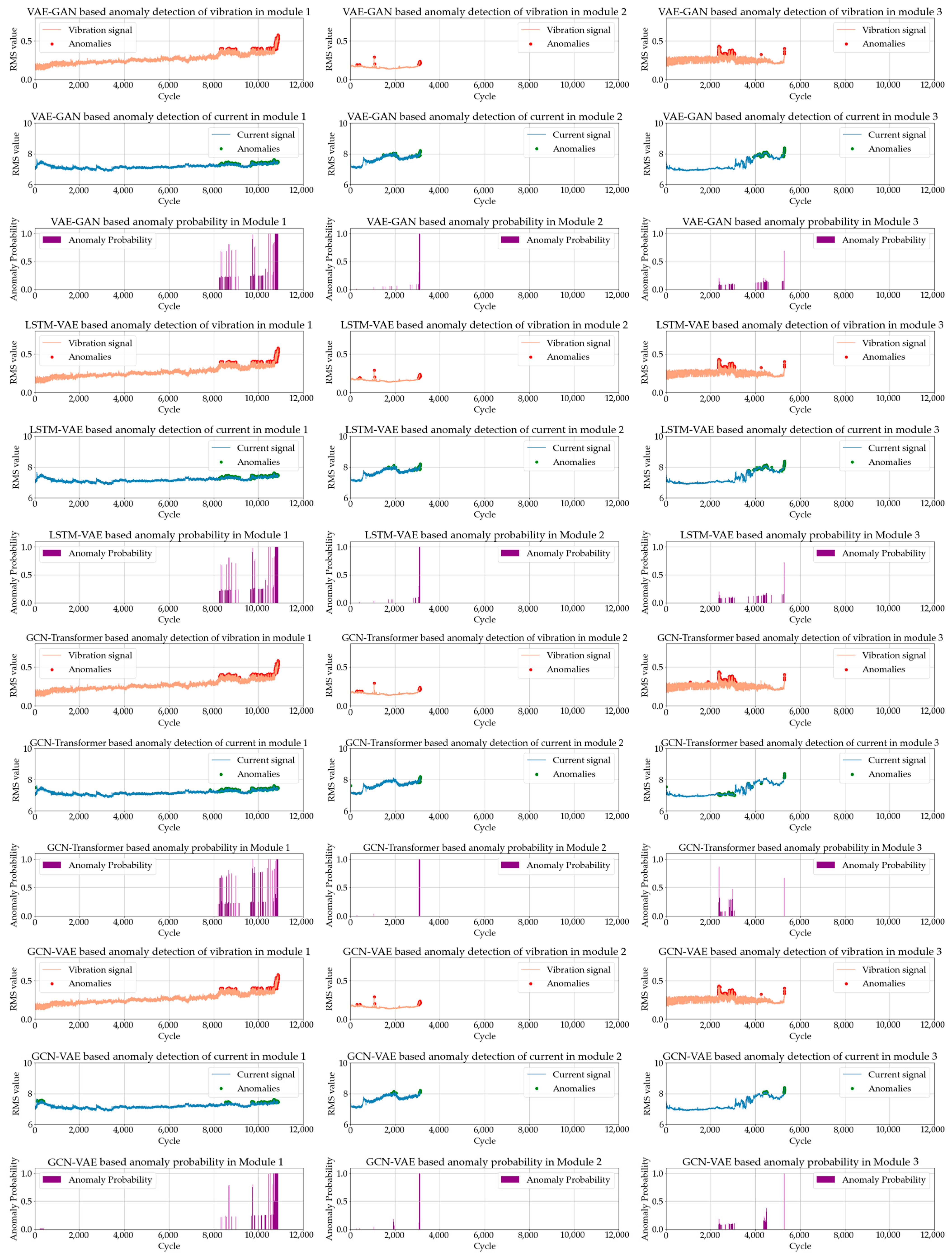
  • In Module 1, all models effectively detected anomalies in the latter part of the data, with particularly strong performance observed from 50 cycles before failure, where all models achieved an anomaly score of 1. At the 200-cycle mark, the ranking of anomaly scores was as follows: GCN-VAE, GCN-Transformer, VAE-GAN, and LSTM-VAE. The superior performance of the proposed GCN-VAE model can be attributed to its ability to effectively leverage both spatial and temporal dependency features. Although the GCN-Transformer model also demonstrated strong performance, the integration of VAE’s reconstruction-based anomaly detection likely provided the GCN-VAE model with a distinct advantage in identifying subtle pre-failure anomalies.
  • In Module 2, the GCN-Transformer model recorded slightly higher anomaly scores compared to the other three models up to 100 cycles before failure. However, as the data approached failure (50, 20, and 10 cycles before failure), all deep learning models achieved an anomaly score of 1, demonstrating robust detection performance. This indicates that all models effectively detect anomalies as the system nears failure. Additionally, the GCN-VAE model consistently maintained high performance throughout, confirming its capability to detect subtle warning signs even in the earlier cycles leading up to failure.
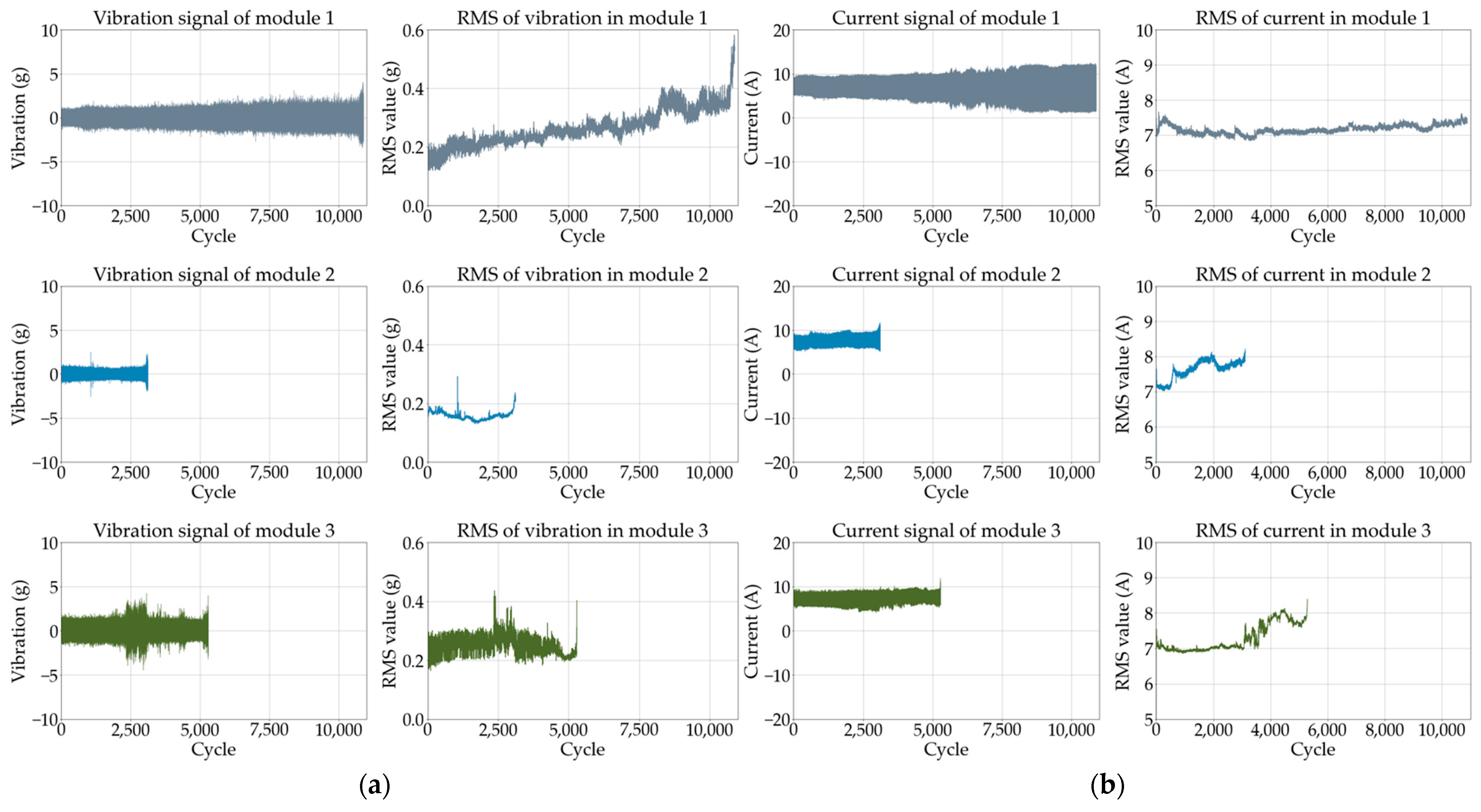
  • In Module 3, all deep learning models exhibited relatively lower anomaly scores compared to Modules 1 and 2, with weaker performance observed even in the pre-failure region. This reduced performance can be attributed to the original signals in Module 3, which exhibited higher noise levels and complex distortions compared to Modules 1 and 2, making anomaly detection more challenging. At 10 cycles before failure, the anomaly scores were ranked as follows: GCN-VAE, LSTM-VAE, VAE-GAN, and GCN-Transformer. The GCN-Transformer effectively modeled spatial and temporal dependencies through its graph and attention mechanisms but lacked a reconstruction-based approach, limiting its ability to detect subtle anomalies. In contrast, the GCN-VAE model consistently achieved the highest anomaly scores across all pre-failure cycles. By leveraging its reconstruction-based capabilities, the GCN-VAE model demonstrated robust and superior anomaly detection performance, even in challenging conditions characterized by high noise levels and complex data distributions.
The experimental results across all three modules consistently highlight the robustness and effectiveness of the proposed GCN-VAE model in detecting anomalies. Its consistent outperformance of other deep learning models, particularly in pre-failure regions, underscores its strong anomaly detection capabilities. This superior performance can be attributed to several key characteristics of the GCN-VAE model:
  • Integration of Spatial and Temporal Dependencies: The GCN component effectively captures spatial and relational features by modeling interactions between data points through graph structures. By incorporating temporal dependencies, the model is able to identify subtle patterns in time-series data that are critical for early anomaly detection. This integration enables the GCN-VAE model to learn complex relationships that may be overlooked by traditional approaches.
  • Reconstruction-Based Anomaly Detection: The VAE component adds a critical layer of sensitivity by learning the underlying distribution of normal data and identifying deviations through reconstruction errors. This mechanism is particularly advantageous in pre-failure scenarios, where subtle anomalies may remain undetected by other models. The combination of VAE’s reconstruction-based approach with GCN’s feature extraction provides the GCN-VAE model with an edge in accurately detecting early fault indicators.
  • Adaptability to Challenging Data Distributions: The experimental results, especially in Module 3, demonstrate the GCN-VAE model’s robustness in handling complex and noisy datasets. While other models showed reduced performance under such conditions, the GCN-VAE model consistently achieved high anomaly scores, reflecting its adaptability and effectiveness in varying data environments.
The GCN-VAE model demonstrated superior performance in anomaly detection across all modules compared to the GCN-Transformer, VAE-GAN, and LSTM-VAE models. This performance is attributed to the synergistic effect created by combining GCN’s graph-based relational learning with VAE’s reconstruction-driven anomaly detection, which is believed to make the GCN-VAE model highly effective in detecting anomalies prior to failure.

5. Conclusions

In this paper, we proposed a GCN-VAE-based anomaly detection method using time-series vibration and current data from durability tests of driving modules in industrial robots and mechanical systems. Traditional fault diagnosis models primarily rely on labeled data for fault detection, but in real industrial environments, obtaining sufficient fault data is challenging due to diverse operating conditions and environmental variations. To address this limitation, we introduced a semi-supervised GCN-VAE model capable of detecting abnormal patterns using only normal data. The GCN-VAE model was employed to accurately detect subtle anomaly signals by extracting spatial features while incorporating temporal continuity and inter-data relationships. These features were then mapped into a latent space, allowing for the detection of abnormal patterns through reconstruction errors. Furthermore, weights were applied to reflect the progression of time and the continuity of anomalies, enhancing the model’s effectiveness in detecting pre-failure anomalies. The experimental results confirmed that the proposed GCN-VAE model outperformed existing hybrid deep learning models, such as VAE-GAN, LSTM-VAE, and GCN-Transformer. These findings demonstrate that the GCN-VAE model possesses robustness and superior anomaly detection capabilities, effectively identifying subtle pre-failure anomalies even in complex and noisy industrial datasets.
While this study demonstrated the effectiveness of the proposed GCN-VAE model, it relied on private data from durability tests of driving modules, which poses limitations in terms of generalizability. To address this, we are actively pursuing ongoing research projects to obtain more diverse and generalized datasets under various conditions. Future work will focus on validating the proposed algorithm using these broader datasets to ensure its robustness and applicability in industrial environments. Additionally, we plan to incorporate data from robotic systems operating in real-world industrial settings, assess the model’s scalability, and explore potential integrations with other AI techniques. These efforts are expected to further enhance the ability to detect diverse anomaly signals and contribute to failure prevention and improved system stability.

Author Contributions

Conceptualization, S.-H.C. and S.L.; funding acquisition, S.L.; investigation, S.-H.C. and D.A.; methodology, S.-H.C., D.A. and I.L.; software, S.-H.C.; visualization, S.-H.C.; writing—original draft, S.-H.C. and S.L.; writing—review and editing, S.L. and I.L. All authors have read and agreed to the published version of the manuscript.

Funding

This work was supported by the Industrial Technology Innovation Program (RS-2024-00422721, Development of safe and reliable XAI-based robotic workcell safety sensors and control modules) funded by the Ministry of Trade, Industry Energy (MOTIE, Korea). This study has been conducted with the support of the Korea Institute of Industrial Technology as “Development of Core Technologies for a Working Partner Robot in the Manufacturing Field (kitech EO-24-0007)”.

Institutional Review Board Statement

Not applicable.

Informed Consent Statement

Not applicable.

Data Availability Statement

The data used in this paper were collected through experiments supported by the project we conducted. Currently, it is difficult to disclose the data for additional experiments and research. In the future, we will strive to share our data by securing more data and conducting further research.

Acknowledgments

The authors appreciate Jongbum Park, Tae-Keun Kim, and Byungjin Jung from the Intelligent Robotics Research Center at the Korea Electronics Technology Institute for their help with this research.

Conflicts of Interest

The authors declare no conflict of interest.

References

  1. Rousopoulou, V.; Vafeiadis, T.; Nizamis, A.; Iakovidis, I.; Samaras, L.; Kirtsoglou, A.; Georgiadis, K.; Ioannidis, D.; Tzovaras, D. Cognitive analytics platform with AI solutions for anomaly detection. Comput. Ind. 2022, 134, 103555. [Google Scholar] [CrossRef]
  2. Vincent, M.; Thomas, S.; Suresh, S.; Prathap, B.R. Enhancing Industrial Equipment Reliability: Advanced Predictive Maintenance Strategies Using Data Analytics and Machine. In Proceedings of the IEEE International Conference on Contemporary Computing and Communications, Bangalore, India, 15–16 March 2024. [Google Scholar]
  3. Serradilla, O.; Zugasti, E.; Okariz, J.R.; Rodriguez, J.; Zurutuza, U. Adaptable and Explainable Predictive Maintenance: Semi-Supervised Deep Learning for Anomaly Detection and Diagnosis in Press Machine Data. App. Sci. 2021, 11, 7376. [Google Scholar] [CrossRef]
  4. Kumar, P.; Khalid, S.; Kim, H.S. Prognostics and Health Management of Rotating Machinery of Industrial Robot with Deep Learning Applications-A Review. Mathematics 2023, 11, 3008. [Google Scholar] [CrossRef]
  5. Deng, C.; Deng, Z.; Lu, S.; He, M.; Miao, J.; Peng, Y. Fault Diagnosis Method for Imbalanced Data Based on Multi-Signal Fusion and Improved Deep Convolution Generative Adversarial Network. Sensors 2023, 23, 2542. [Google Scholar] [CrossRef] [PubMed]
  6. Ren, Z.; Lin, T.; Feng, K.; Zhu, Y.; Liu, Z.; Yan, K. A Systematic Review on Imbalanced Learning Methods in Intelligent Fault Diagnosis. IEEE Trans. Instrum. Meas. 2023, 72, 3508535. [Google Scholar] [CrossRef]
  7. Soori, M.; Dastres, R.; Arezoo, B.; Jough, F.K.G. Intelligent robotic systems in Industry 4.0: A review. J. Adv. Manuf. Sci. Technol. 2024, 4, 2024007. [Google Scholar]
  8. Monteiro, R.P.; Lozada, M.C.; Mendieta, D.R.C.; Loja, R.V.S.; Filho, C.J.A.B. A hybrid prototype selection-based deep learning approach for anomaly detection in industrial machines. Expert Syst. Appl. 2022, 204, 117528. [Google Scholar] [CrossRef]
  9. Ahmed, I.; Ahmed, M.; Chehri, A.; Jeon, G. A Smart-Anomaly-Detection System for Industrial Machines Based on Feature Autoencoder and Deep Learning. Micromachines 2023, 14, 154. [Google Scholar] [CrossRef] [PubMed]
  10. Webert, H.; Döß, T.; Kaupp, L.; Simons, S. Fault Handling in Industry 4.0: Definition, Process and Applications. Sensors 2022, 22, 2205. [Google Scholar] [CrossRef] [PubMed]
  11. Kumar, P.; Raouf, I.; Kim, H.S. Transfer learning for servomotor bearing fault detection in the industrial robot. Adv. Eng. Softw. 2024, 194, 103672. [Google Scholar] [CrossRef]
  12. Sabry, A.H.; Amirulddin, U.A.B.U. A review on fault detection and diagnosis of industrial robots and multi-axis machines. Results Eng. 2024, 23, 102397. [Google Scholar] [CrossRef]
  13. Graabæk, S.G.; Ancker, E.V.; Fugl, A.R.; Christensen, A.L. An Experimental Comparison of Anomaly Detection Methods for Collaborative Robot Manipulators. IEEE Access 2023, 11, 65834–65848. [Google Scholar] [CrossRef]
  14. Deng, C.; Song, J.; Chen, C.; Wang, T.; Cheng, L. Semi-Supervised Informer for the Compound Fault Diagnosis of Industrial Robots. Sensors 2024, 24, 3732. [Google Scholar] [CrossRef] [PubMed]
  15. Gao, Y.; Liu, Y.; Jin, Y.; Chen, J.; Wu, H. A Novel Semi-Supervised Learning Approach for Network Intrusion Detection on Cloud-Based Robotic System. IEEE Access 2018, 6, 50927–50938. [Google Scholar] [CrossRef]
  16. Cohen, J.; Ni, J. Semi-Supervised Learning for Anomaly Classification Using Partially Labeled Subsets. J. Manuf. Sci. Eng. 2022, 144, 061008. [Google Scholar] [CrossRef]
  17. Zhu, Y.; Wang, M.; Yin, X.; Zhang, J.; Meijering, E.; Hu, J. Deep Learning in Diverse Intelligent Sensor Based Systems. Sensors 2023, 23, 62. [Google Scholar] [CrossRef]
  18. Choi, K.; Yi, J.; Park, C.; Yoon, S. Deep Learning for Anomaly Detection in Time-Series Data: Review, Analysis, and Guidelines. IEEE Access 2021, 9, 120043–120065. [Google Scholar] [CrossRef]
  19. He, Q.; Wang, G.; Wang, H.; Chen, L. Multivariate time-series anomaly detection via temporal convolutional and graph attention networks. J. Intell. Fuzzy Syst. 2023, 44, 5953–5962. [Google Scholar] [CrossRef]
  20. Fan, Z.; Wang, Y.; Meng, L.; Zhang, G.; Qin, Y.; Tang, B. Unsupervised Anomaly Detection Method for Bearing Based on VAE-GAN and Time-Series Data Correlation Enhancement. IEEE Sens. J. 2023, 23, 29345–29356. [Google Scholar] [CrossRef]
  21. Ou, X.; Wen, G.; Huang, X.; Su, Y.; Chen, X.; Lin, H. A deep sequence multi-distribution adversarial model for bearing abnormal condition detection. Measurement 2021, 182, 109529. [Google Scholar] [CrossRef]
  22. Yang, G.; Tao, H.; Du, R.; Zhong, Y. Compound Fault Diagnosis of Harmonic Drives Using Deep Capsule Graph Convolutional Network. IEEE Trans. Ind. Electron. 2023, 70, 4189–4195. [Google Scholar] [CrossRef]
  23. Yan, J.; Cheng, Y.; Wang, Q.; Liu, L.; Zhang, W.; Jin, B. Transformer and Graph Convolution-Based Unsupervised Detection of Machine Anomalous Sound Under Domain Shifts. IEEE Trans. Emerg. Top. Comput. Intell. 2024, 8, 2827–2842. [Google Scholar] [CrossRef]
  24. Jin, M.; Koh, H.Y.; Wen, Q.; Zambon, D.; Alippi, C.; Webb, G.I.; King, I.; Pan, S. A Survey on Graph Neural Networks for Time Series: Forecasting, Classification, Imputation, and Anomaly Detection. arXiv 2024, arXiv:2307.03759v3. [Google Scholar] [CrossRef] [PubMed]
  25. Nguyen, H.H.; Nguyen, C.N.; Dao, X.T.; Duong, Q.T.; Kim, D.P.T.; Pham, M.T. Variational Autoencoder for Anomaly Detection: A Comparative Study. arXiv 2024, arXiv:2408.13561v1. [Google Scholar]
  26. Collin, T.; Kindlmann, G.; Scott, L.R. An Adaptive Savitsky-Golay Filter for Smoothing Finite Element Computation. arXiv 2019, arXiv:1911.00790v2. [Google Scholar]
  27. Ochieng, P.J.; Maróti, Z.; Dombi, J.; Krész, M.; Békési, J.; Kalmár, T. Adaptive Savitzky–Golay Filters for Analysis of Copy Number Variation Peaks from Whole-Exome Sequencing Data. Information 2023, 14, 128. [Google Scholar] [CrossRef]
  28. Yun, H.; Kim, H.; Jeong, Y.H.; Martin, J.B.G. Autoencoder-based anomaly detection of industrial robot arm using stethoscope-based internal sound sensor. J. Intell. Manuf. 2023, 34, 1427–1444. [Google Scholar] [CrossRef]
  29. Jung, Y.; Park, E.G.; Jeong, S.H.; Kim, J.H. AI-Based Anomaly Detection Techniques for Structural Fault Diagnosis Using Low-Sampling-Rate Vibration Data. Aerospace 2024, 11, 509. [Google Scholar] [CrossRef]
  30. Wang, F.; Wang, K.; Yao, B. Time series anomaly detection with reconstruction-based state-space models. arXiv 2023, arXiv:2303.03324v3. [Google Scholar]
  31. Sun, S.; Ding, H. Fault Feature Extraction Based on Unsupervised Graph Embedding for Harmonic Reducers Diagnosis. In The 2nd International Conference on Mechanical System Dynamics; Springer: Singapore, 2023; pp. 3375–3389. [Google Scholar]
  32. Chen, Z.; Xu, J.; Alippi, C.; Ding, S.X.; Shardt, Y.; Peng, T.; Yang, C. Graph neural network-based fault diagnosis: A review. arXiv 2021, arXiv:2111.08185. [Google Scholar]
  33. Kipf, T.N.; Welling, M. Semi-Supervised Classification with Graph Convolutional Networks. arXiv 2017, arXiv:1609.02907v4. [Google Scholar]
  34. Zhang, S.; Ye, F.; Wang, B.; Habetler, T.G. Semi-Supervised Learning of Bearing Anomaly Detection via Deep Variational Autoencoders. arXiv 2019, arXiv:1912.01096v2. [Google Scholar]
  35. Ghanim, J.; Issa, M.; Awad, M. An Asymmetric Loss with Anomaly Detection LSTM Framework for Power Consumption Prediction. arXiv 2023, arXiv:2302.10889. [Google Scholar]
  36. Baidya, R.; Jeong, H. Anomaly Detection in Time Series Data Using Reversible Instance Normalized Anomaly Transformer. Sensors 2023, 23, 9272. [Google Scholar] [CrossRef]
  37. Li, J.; Izakian, H.; Pedrycz, W.; Jamal, I. Clustering-based anomaly detection in multivariate time series data. Appl. Soft Comput. J. 2021, 100, 106919. [Google Scholar] [CrossRef]
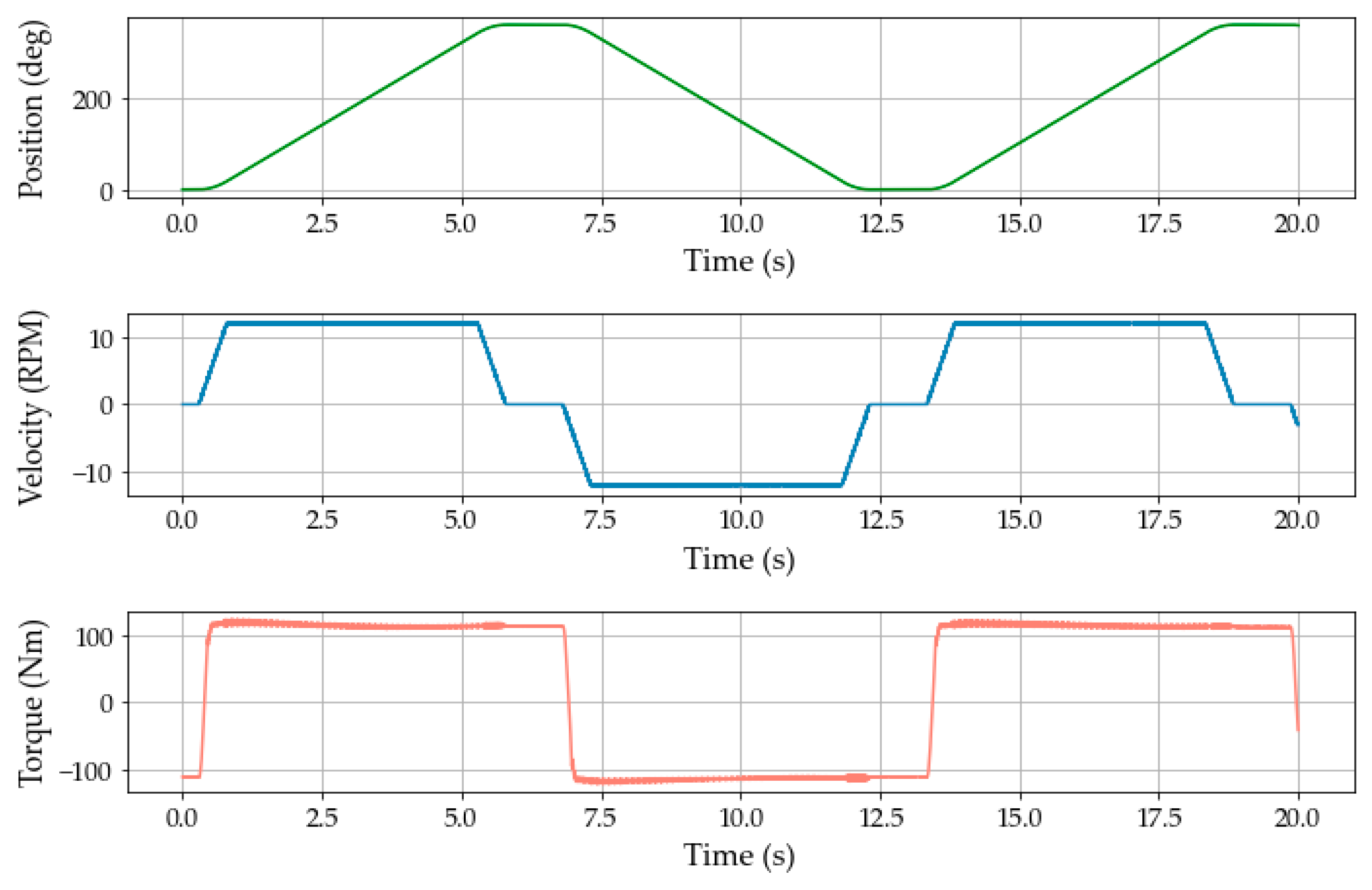
Figure 1. Experimental platform (driving module with forward rotation).
Mathematics 12 03750 g001
Figure 2. Experimental conditions and methods of the driving modules in the durability test.
Mathematics 12 03750 g002
Figure 3. Raw data and RMS values for vibration and current signals of the driving modules. (a) Vibration signal and RMS values. (b) Current signal and RMS values
Mathematics 12 03750 g003
Figure 4. Anomaly detection results based on statistical features.
Mathematics 12 03750 g004
Figure 5. Anomaly detection results according to the learning model of vibration data.
Mathematics 12 03750 g005
Figure 6. Anomaly detection results according to the learning model of current data.
Mathematics 12 03750 g006
Figure 7. An anomaly detection algorithm based on GCN-VAE.
Mathematics 12 03750 g007
Figure 8. Comparison of anomaly detection results based on hybrid deep learning models for vibration and current data.
Mathematics 12 03750 g008
Table 1. Experiment condition for durability test of the driving module.
TorqueConst.
Velocity
Acc/Dec VelocityConst. Velocity TimeAcc/Dec TimeStop TimeCycle
113 Nm12 RPM24 RPM/s24.5 s0.5 s1 s13 s
Table 2. Anomaly detection matching accuracy of the statistical features and learning models.
Train ModuleTest ModuleDataMatching Accuracy of Statistical Features and Learning Models (%)
AnoGANLSTMVAETransformerGCN
1, 23Vibration98.941898.715099.319799.395399.3197
Current96.164096.315296.315296.315299.6788
1, 32Vibration96.342699.294299.422599.422599.4225
Current96.374798.492198.684699.390499.9038
2, 31Vibration99.070299.070299.231199.301899.3018
Current98.936198.900399.275899.292699.0170
AverageVibration98.118299.026599.324599.373299.3480
Current97.158397.902598.085998.332799.5332
Table 3. Comparison of anomaly detection performance based on anomaly scores.
Test ModuleModelAnomaly Scores for Pre-Failure Cycles
Total Cycle500 Cycle200 Cycle100 Cycle50 Cycle20 Cycle10 Cycle
1VAE-GAN0.02210.35340.76641.00001.00001.00001.0000
LSTM-VAE0.02190.34610.75091.00001.00001.00001.0000
GCN-Trans0.01860.50180.82171.00001.00001.00001.0000
GCN-VAE0.02220.42310.87761.00001.00001.00001.0000
2VAE-GAN0.01750.10630.26480.52681.00001.00001.0000
LSTM-VAE0.01690.10350.25750.51401.00001.00001.0000
GCN-Trans0.01850.11500.28750.57511.00001.00001.0000
GCN-VAE0.01800.10320.25810.51611.00001.00001.0000
3VAE-GAN0.00540.00930.02330.04510.07810.17260.3149
LSTM-VAE0.00540.01150.02880.05200.09450.22100.3799
GCN-Trans0.00700.00580.01440.02890.05770.14430.2885
GCN-VAE0.00770.02010.05030.10060.20120.50290.7029
Disclaimer/Publisher’s Note: The statements, opinions and data contained in all publications are solely those of the individual author(s) and contributor(s) and not of MDPI and/or the editor(s). MDPI and/or the editor(s) disclaim responsibility for any injury to people or property resulting from any ideas, methods, instructions or products referred to in the content.

