Portfolio Selection Based on Modified CoVaR in Gaussian Framework

Abstract

We study a Mean-Risk model, where risk is measured by a Modified CoVaR (Conditional Value at Risk): ${CoVaR}_{\alpha ,\beta }^{\le }\left(X\right|Y)=Va{R}_{\beta }\left(X\right|Y+Va{R}_{\alpha }\left(Y\right)\le 0).$ We prove that in a Gaussian setting, for a sufficiently small $\beta$, such a model has a solution. There exists a portfolio that fulfills the given constraints and for which the risk is minimal. This is shown in relation to the mean–standard deviation portfolio, and numerical examples are provided.

1. Introduction

The question of optimal asset allocation is as old as the history of investing itself, yet the pioneering work of Markowitz is barely over seventy years old, and it was as recent as 1990 that the Alfred Nobel Memorial Prize in Economic Sciences was awarded for the theory of portfolio choice (Harry Markowitz), the Capital Asset Pricing Model (William Sharpe), and the theory of corporate finance (Merton Miller). There are still ample opportunities to explore interesting questions inside the complex field of portfolio analysis. The model allowing for the possibility of short-selling is known as the Black model—see [1] and the original article of [2]. The mutual fund theorem in [3] shows that in a world of risky assets and one riskless security, using a quadratic utility function (or two-parameter distribution of returns), an investor will inevitably choose a given linear combination of exactly two portfolios, one known as the tangency portfolio, maximizing the Sharpe Ratio, and the other consisting exclusively of the risk-free asset. The poor performance of the Markowitz model fed with sample moments has not only been discussed but has also been handled in various ways, from using an empirical Bayes approach (e.g., [4]), posing constraints (e.g., [5]), or altering the weights of historical data (among the most recent is [6]) to using a model factoring in predictions of the investors, as implemented by [7], among others (see [8] for step-by-step instructions or [9] for ‘general continuous distributions and deviation measures of risk’). These approaches generally take into account the surprising fact that sample covariance might perform quite well, while the sample mean is rather worthless—see the superb discussion provided by [10] on the subject. We will pursue a path of investigating the Conditional Value at Risk (CoVaR for short), which is selected instead of variance as the risk measure in the Markowitz model. The task before us is to find the portfolio with the lowest risk simultaneously retaining the chosen expected return and stressing one of the variables. The risk measure we have chosen originated in 2008 in the technical report by Adrian and Brunnermeier, was expanded on in a 2011 report [11], and has gained recognition so quickly that it has accumulated a staggering number of citations—over 4600. Over $95\%$ of these preceded the official paper [12]. This highlights how much the new risk measure was sought after and appreciated, as well as the importance of the possibility of having one of the variables under distress while calculating the overall Value-at-Risk (wildly popular itself and promoted by Basel II Accord), especially after the global financial crisis of 2007–2009 (discussed in [12]).

To fix the notation, in this paper, we will base our approach on the Profit/Loss (P/L) approach used in, for example, [12,13,14,15,16,17].

We will study random variables X and Y, which can model, for example, the welfare of financial institutions, financial positions, gains of investments, or rates of returns of stock prices and indices. So, generally,

“The higher the value of X, the better”.

The above can be expressed in terms of quantiles. Namely, Value-at-Risk at a significance level $\alpha$ is equal to the minus upper $\alpha$ quantile of X or lower $1-\alpha$ quantile of the loss, $-X$.

$$Va{R}_{\alpha }\left(X\right)=-Q_{\alpha }^{+}\left(X\right)=Q_{1-\alpha }^{-}(-X).$$

We recall that for a given random variable X and a given level $\kappa \in (0,1)$, the set of $\kappa$ quantiles is a closed interval $Q_{\kappa }\left(X\right)$, which might be reduced to a point. The end points of the interval $Q_{\kappa }\left(X\right)$ are referred to as upper and lower quantiles.

$$[Q_{\kappa }^{-}\left(X\right),Q_{\kappa }^{+}\left(X\right)]=Q_{\kappa }\left(X\right)=\{x:\mathbb{P}(X\le x)\ge \kappa \mathrm{and}\mathbb{P}(X\ge x)\ge 1-\kappa \}.$$

To switch to the alternative Loss/Profit (L/P) approach (applied, for example, in [18,19,20]), when random variables are modeling losses in financial investments, actuarial risks, or high water levels in hydrology, it is enough to change the sign of the variables:

$$L=-X,$$

Remember that, by convention, the subscript is changed. The significance level $\alpha$ is replaced by the confidence level $c=1-\alpha$:

$$Va{R}_c\left(L\right)=Va{R}_{\alpha }\left(X\right).$$

Now, assume that we are measuring the risk given some stress event. For example, we want to determine how big a bailout would be necessary to keep a financial institution X solvent with a probability at least $1-\beta$ if a financial institution Y was to perform badly. The Conditional Value-at-Risk (CoVaR) by Adrian and Brunnermeier and its later modifications prove to be very useful tools for measuring (quantifying) such phenomena.

Let X and Y be random variables modeling positions. CoVaR is defined as the VaR of X conditioned by Y. In more detail,

$$CoVaR\left(X\right|Y)=Va{R}_{\beta }\left(X\right|Y\in \mathcal{E}),$$

where a Borel subset of the real line $\mathcal{E}$ is modeling some adverse event concerning Y. Most often, $\mathcal{E}$ consists of one point (a threshold) or is a half-line bounded by a threshold.

As we see, to deal with CoVaR, one has to model the dependence between X and Y. This can be achieved by means of copulas, as can be seen in [13,15,16].

Adrian and Brunnermeier [12] applied a construction with E consisting of one point. Such an approach has a certain drawback, as pointed out, for example, by Mainik and Schaanning in [20], which is due to the fact that the standard CoVaR is not compatible with a concordance ordering. Hence, it is “breaking” the following paradigm: more dependence, more systemic risk (see also [15]). To avoid this inconsistency, a modified definition of CoVaR was introduced in 2013 and 2014 by Girardi and A.T. Ergün [21] and by Mainik and Schaanning [20], both in an L/P setting.

The modified Conditional VaR at a level $(\alpha ,\beta )$, which is a main objective of this survey, is defined as the VaR at level $\beta$ of X under the condition that $Y\le -Va{R}_{\alpha }\left(Y\right)$.

In this survey, we consider the portfolio optimization problem with risk measured by the modified CoVaR under the assumption of the normality of returns. It is shown that a switch from the “standard” CoVaR with one pointed $\mathcal{E}$ (see [17]) to the modified CoVaR makes the problem more demanding. For example, in the “modified” problem, it is not obvious that between portfolios having fixed and expected values, one can find a portfolio minimizing risk.

This paper is organized in the following way:

In Section 2, “Notation”, we recall the basics about CoVaR and portfolio selection. In the next section, “The Mean-CoVaR model”, we present our main results concerning the existence of optimal portfolios. The following section, “Proofs and auxiliary results”, deals with Gaussian copulas and optimization problems. In the last section, we provide numerical results concerning a given four-dimensional portfolio.

2. Notation

2.1. CoVaR in Copula Setting

We present the following definition based on [13].

Definition 1.

$${CoVaR}_{\alpha ,\beta }^{\le }\left(X\right|Y)=Va{R}_{\beta }\left(X\right|Y\le -Va{R}_{\alpha }\left(Y\right)),$$

(1)

which can be expressed in terms of quantiles:

$${CoVaR}_{\alpha ,\beta }^{\le }\left(X\right|Y)=-Q_{\beta }^{+}\left(X\right|Y\le Q_{\alpha }^{+}\left(Y\right)).$$

We assume that the distribution functions of Y and X ($F_Y$ and $F_X$) are continuous and their joint distribution is described by a copula C (for more details about copulas, the reader is referred to to the monograph of Roger Nelsen [22] or other publications on the subject like [23,24,25,26,27]).

From the aforementioned article [13], we learn that, since

$$\mathbb{P}(X\le x|Y\le Q_{\alpha }^{+}\left(Y\right))={\displaystyle \frac{\mathbb{P}(X\le x,Y\le Q_{\alpha }^{+}\left(Y\right))}{\alpha }}={\displaystyle \frac{C(\alpha ,F_X\left(x\right))}{\alpha }},$$

the following is valid:

Theorem 1.

For fixed α and $\beta \in (0,1)$, we obtain

$${CoVaR}_{\alpha ,\beta }^{\le }\left(X\right|Y)={VaR}_w\left(X\right),$$

(2)

where w is the maximal root of the following equation:

$$C(\alpha ,w)=\alpha \beta .$$

(3)

For more details, the reader is referred to [15,16].

When, furthermore, we assume that the pair $(X,Y)$ is normally distributed, then

$$\begin{array}{ccc}\hfill {CoVaR}_{\alpha ,\beta }^{\le }\left(X\right|Y)& =& -\mathbb{E}\left(X\right)-{\mathsf{\Phi }}^{-1}\left(w\right)\sigma \left(X\right),\hfill \end{array}$$

(4)

and

$$\begin{array}{ccc}\hfill C(\alpha ,w,\rho (X,Y\left)\right)& =& \alpha \beta ,\hfill \end{array}$$

(5)

where $C(u,v,\rho )$ denotes a Gaussian copula with a parameter (correlation coefficient) $\rho$, $\mathsf{\Phi }$ is a distribution function of a univariate standard normal probability law ${\mathcal{N}}_1(0,1)$, $\mathbb{E}$ is the expected value, and $\sigma$ denotes the standard deviation. Thus, the impact of Y is encapsulated in the correlation coefficient. The implied significance level w is a function of $\alpha ,\beta$, and $\rho$.

$$w=w(\alpha ,\beta ,\rho ),$$

which is decreasing with $\rho$.

$$w(\alpha ,\beta ,-1)=1-\alpha (1-\beta ),w(\alpha ,\beta ,0)=\beta ,w(\alpha ,\beta ,1)=\alpha \beta .$$

Furthermore, $\rho$ depends on X. For more details, see Section 4.1.

2.2. Portfolio Selection

A portfolio (i.e., investment strategy) $x={(x_1,\dots ,x_n)}^T$ meets the natural condition of summing up to 1, and $\mu ={({\mu }_1,\dots ,{\mu }_n)}^T$ is defined as the expected value of n-dimensional random variable of returns on risky assets, $R={(R_1,\dots ,R_n)}^T$. Now, we add the assumption of normality of R, which is made throughout the rest of the article. To obtain a non-degenerate problem, two more assumptions are made. First, $\mu \nparallel {\mathbb{1}}_n={(1,\dots ,1)}^T$; i.e., not every asset has the same expected return. Second, the covariance matrix of R, $\mathsf{\Sigma }={\left[{\sigma }_{ij}\right]}_{i,j=1,\dots ,n}$, is positive definite.

We also define $X=x^{T}R={\displaystyle \sum _{i=1}^n}{x}_i{R}_i$, the univariate random variable of return on the portfolio. Obviously, the expected value and the variance are given by

$$\mathbb{E}\left(X\right)=\mathbb{E}\left(x^{T}R\right)=x^T\mu ,$$

$${\sigma }^2\left(X\right)={\sigma }^2\left(x^{T}R\right)=x^T\mathsf{\Sigma }x={\left|\right|x\left|\right|}_{\mathsf{\Sigma }}^2.$$

The distribution of X is conditioned on one chosen variable $R_i$, $i\in \{1,\dots ,n\}$. Without loss of generality, let that be $Y=R_1$. The correlation coefficient $\rho =\rho (X,R_1)$ (provided $X\ne 0$) is equal to the cosine of the angle between vectors x and $e_1$ in the metric in ${\left(R\right)}^n$ induced by the scalar product given by the matrix $\mathsf{\Sigma }$:

$$\rho =\sigma {\left(X\right)}^{-1}\sigma {\left(R_1\right)}^{-1}cov(X,R_1)={\displaystyle \frac{e_1^T\mathsf{\Sigma }x}{\sqrt{e_1^T\mathsf{\Sigma }{e}_1}\sqrt{x^T\mathsf{\Sigma }x}}}={cos}_{\mathsf{\Sigma }}(x,e_1)$$

(6)

where $e_1={(1,0,\dots ,0)}^T$.

We select portfolios with respect to two criteria. We maximize the expected value and minimize the risk measured by CoVaR.

We recall that a portfolio x, $x^T{\mathbb{1}}_n=1$ is called efficient if and only if it is maximal with respect to the generalized Markowitz ordering, which means that there exists no portfolio y fulfilling the budget constraints $y^T{\mathbb{1}}_n=1$, such that

$$\mathbb{E}\left(y^{T}R\right)\ge \mathbb{E}\left(x^{T}R\right)\mathrm{and}{CoVaR}_{\alpha ,\beta }^{\le }(y^{T}R\mid R_1)\le {CoVaR}_{\alpha ,\beta }^{\le }(x^{T}R\mid R_1)$$

(7)

where at least one inequality is strict.

3. The Mean-CoVaR Model

First, we want to find the portfolio x with a fixed return that minimizes CoVaR. The optimization problem for x presents itself as follows:

$$\left\{\begin{array}{c}{CoVaR}_{\alpha ,\beta }^{\le }(x^{T}R\mid R_1)\to min,\hfill \\ x^T\mu =E,\hfill \\ x^T{\mathbb{1}}_n=1,\hfill \end{array}\right.$$

(8)

where R is normally distributed, $R\sim {\mathcal{N}}_n(\mu ,\mathsf{\Sigma })$. For a given E, $\mu$, and $\mathsf{\Sigma }$, seek the one that minimizes the target function among the xs fulfilling the constraints.

The solution of the above problem is closely related to the classical Markowitz problem:

$$\left\{\begin{array}{c}{x}^T\mathsf{\Sigma }x\to min\hfill \\ x^T\mu =E\hfill \\ x^T{\mathbb{1}}_n=1\hfill \end{array}\right.$$

(9)

We recall that this problem has a unique solution $X_M\in {\mathbb{R}}^n$ when the following hold:

• The symmetric matrix $\mathsf{\Sigma }$ is positively defined, i.e., is a matrix of a scalar product on ${\mathbb{R}}^n$;
• The vectors $\mu$ and ${\mathbb{1}}_n$ are linearly independent (i.e., not parallel);
• E is any real number.

The solution $X_M$ is given by the following formula:

$$X_M^T\left(E\right)=(E,1)G^{-1}{(\mu ,{\mathbb{1}}_n)}^T{\mathsf{\Sigma }}^{-1},$$

(10)

where G is a Gram matrix of vectors $\mu$ and ${\mathbb{1}}_n$ with respect to the scalar product defined by the matrix ${\mathsf{\Sigma }}^{-1}$, which is to say

$$G={(\mu ,{\mathbb{1}}_n)}^T{\mathsf{\Sigma }}^{-1}(\mu ,{\mathbb{1}}_n),$$

(11)

where $(\mu ,{\mathbb{1}}_n)$ denotes an $n\times 2$ matrix with columns $\mu$ and ${\mathbb{1}}_n$. For details, see Section 4.2.2.

The existence of the solution $X_{*}$ of the optimization problem (8) depends on portfolio $X_{\infty }$, given by the following formula:

$$X_{\infty }^T=e_1^T-X_M^T\left({\mu }_1\right)=e_1^T-({\mu }_1,1)G^{-1}{(\mu ,{\mathbb{1}}_n)}^T{\mathsf{\Sigma }}^{-1}.$$

(12)

We recall that ${\mu }_1$, the first coefficient of the vector $\mu$, is equal to $\mathbb{E}\left(Y\right)$. Note that $X_{\infty }$ is orthogonal to vectors $\mu$ and ${\mathbb{1}}_n$ with respect to the standard scalar product and orthogonal to $X_M$ with respect to the scalar product associated with the matrix $\mathsf{\Sigma }$—for proofs, see (49) and (50). In addition, if we define q such that the following is the case:

$$q^T=e_1^T\mathsf{\Sigma }=X_{\infty }^T\mathsf{\Sigma }+\left(({\mu }_1,1)G^{-1}\right){(\mu ,{\mathbb{1}}_n)}^T,$$

(13)

Then, the vanishing of $X_{\infty }$ implies that the vectors $q,\mu ,{\mathbb{1}}_n$ are linearly dependent.

Theorem 2.

For $q,\mu$, and ${\mathbb{1}}_n$, which are linearly independent, the solvability of the optimization problem (8) is as follows:

1. It has no solution when

$$\beta >{\displaystyle \frac{1}{\alpha }}C\left(\alpha ,{\displaystyle \frac{1}{2}},-{cos}_{\mathsf{\Sigma }}(e_1,X_{\infty })\right);$$

2. It has a solution when

$$\beta <{\displaystyle \frac{1}{\alpha }}C\left(\alpha ,{\displaystyle \frac{1}{2}},-{cos}_{\mathsf{\Sigma }}(e_1,X_{\infty })\right);$$

where $C(u,v,\rho )$ is a Gaussian copula with correlation parameter ρ. Moreover, if $X_{*}$ is a solution of the optimization problem (8), then the vector $X_{*}-X_M$ is parallel to $X_{\infty }$.

$$X_{*}=X_M\left(E\right)-\lambda \left(E\right)X_{\infty },$$

(14)

where

$$\lambda \left(E\right)\in {Argmin}_{\lambda \ge 0}\left(-{\mathsf{\Phi }}^{-1}\left(w(\alpha ,\beta ,{cos}_{\mathsf{\Sigma }}(e_1,X_M\left(E\right)-\lambda X_{\infty }))\right)·\sqrt{\left|\right|X_M{\left(E\right)\left|\right|}_{\mathsf{\Sigma }}^2+{\lambda }^2\left|\right|X_{\infty }{\left|\right|}_{\mathsf{\Sigma }}^2}\right).$$

(15)

The proof is provided in Section 4.2.

Remark 1.

For $\beta ={\displaystyle \frac{1}{\alpha }}C\left(\alpha ,{\displaystyle \frac{1}{2}},-{cos}_{\mathsf{\Sigma }}(e_1,X_{\infty })\right)$, a solution of the optimization problem (8) may not exist; see Example 1.

Next, we want to find the portfolio x that minimizes CoVaR. The optimization problem for x presents itself as follows:

$$\left\{\begin{array}{c}{CoVaR}_{\alpha ,\beta }^{\le }(x^{T}R\mid R_1)\to min,\hfill \\ x^T{\mathbb{1}}_n=1,\hfill \end{array}\right.$$

(16)

where $R\sim {\mathcal{N}}_n(\mu ,\mathsf{\Sigma })$.

Let the vector $X_d$ denote the derivative of $X_M\left(E\right)$ with respect to E. Then,

$$X_d^T={\displaystyle \frac{d{X}_M{\left(E\right)}^T}{dE}}=(1,0)G^{-1}{(\mu ,{\mathbb{1}}_n)}^T{\mathsf{\Sigma }}^{-1}$$

(17)

and

$$\left|\right|X_d{\left|\right|}_{\mathsf{\Sigma }}^2=X_d^T\mathsf{\Sigma }{X}_d=(1,0)G^{-1}{(1,0)}^T={\displaystyle \frac{{\mathbb{1}}_n^T{\mathsf{\Sigma }}^{-1}{\mathbb{1}}_n}{det\left(G\right)}}.$$

(18)

Theorem 3.

For $q,\mu ,$ and ${\mathbb{1}}_n$, which are linearly independent, the solvability of the optimization problem (16) is as follows:

1. It has no solution when

$$\beta >min\left({\displaystyle \frac{1}{\alpha }}C\left(\alpha ,\mathsf{\Phi }\left({\displaystyle \frac{-\xi }{\left|\right|X_d{\left|\right|}_{\mathsf{\Sigma }}}}\right),\xi {cos}_{\mathsf{\Sigma }}(e_1,X_d)-\sqrt{1-{\xi }^2}{cos}_{\mathsf{\Sigma }}(e_1,X_{\infty })\right)|\xi \in [0,1]\right);$$

2. It has a solution when

$$\beta <min\left({\displaystyle \frac{1}{\alpha }}C\left(\alpha ,\mathsf{\Phi }\left({\displaystyle \frac{-\xi }{\left|\right|X_d{\left|\right|}_{\mathsf{\Sigma }}}}\right),\xi {cos}_{\mathsf{\Sigma }}(e_1,X_d)-\sqrt{1-{\xi }^2}{cos}_{\mathsf{\Sigma }}(e_1,X_{\infty })\right)|\xi \in [0,1]\right);$$

where $C(u,v,\rho )$ is a Gaussian copula with the correlation parameter ρ.

The proof is provided in Section 4.2.

Remark 2.

Note that when the set of the portfolios of the minimal risk is nonempty and bounded, then the one with the maximal expected value of return is an efficient portfolio. Moreover, the existence of a nonempty, bounded set of portfolios of the minimal risk is a necessary and sufficient condition for the existence of efficient portfolios.

4. Proofs and Auxiliary Results

4.1. Gaussian Copulas

Let us consider a Gaussian Copula:

$$C(u,v;\rho )=\underset{-\infty }{\overset{{\mathsf{\Phi }}^{-1}\left(u\right)}{\int }}\underset{-\infty }{\overset{{\mathsf{\Phi }}^{-1}\left(v\right)}{\int }}{\displaystyle \frac{e^{-\frac{{\xi }^2-2\rho \xi \eta +{\eta }^2}{2\left(1-{\rho }^2\right)}}}{2\pi \sqrt{1-{\rho }^2}}}\mathrm{d}\xi \mathrm{d}\eta .$$

(19)

The correlation coefficient $\rho$ is added to the copula symbol for the convenience of notation as it is the only other parameter needed for the computation of a copula, due to all elliptical copulas being normalization-invariant (c.f. [28], p. 174, Remark 4.3).

Meyer in [29] shows that the Gaussian copula can be extended continuously, approaching the lower and upper Fréchet–Hoeffding bounds, i.e., W and M, respectively; in dimension 2, both of these are copulas.

$$\begin{array}{ccc}\hfill \underset{\rho \to 1}{lim}C(u,v,\rho )& =& min(u,v)=M(u,v),\hfill \end{array}$$

(20)

$$\begin{array}{ccc}\hfill \underset{\rho \to -1}{lim}C(u,v,\rho )& =& max(u+v-1,0)=W(u,v).\hfill \end{array}$$

(21)

Following (c.f. [29]), we obtain an extension of the classical Fréchet–Hoeffding inequality:

Corollary 1.

$$\begin{array}{cc}\hfill & W(u,v)=max\{u+v-1,0\}<C(u,v,{\rho }_1)<C(u,v,0)=uv\hfill \\ \hfill & <C(u,v,{\rho }_2)<M(u,v)=min\{u,v\}\hfill \\ \hfill & where{\rho }_1<0<{\rho }_2.\hfill \end{array}$$

(22)

Remark 3.

The Double Gaussian distribution ${\mathsf{\Phi }}_2$ fulfills the following:

For

$${\varphi }_2(x,y;\rho )={\displaystyle \frac{e^{-\frac{x^2-2\rho xy+y^2}{2\left(1-{\rho }^2\right)}}}{2\pi \sqrt{1-{\rho }^2}}}and{\mathsf{\Phi }}_2(x,y;\rho )=\underset{-\infty }{\overset{y}{\int }}\underset{-\infty }{\overset{x}{\int }}{\varphi }_2(\xi ,\nu ;\rho )\mathrm{d}\xi \mathrm{d}\nu$$

(23)

one has

$${\displaystyle \frac{\partial }{\partial \rho }}{\varphi }_2(x,y;\rho )={\displaystyle \frac{{\partial }^2}{\partial u\partial v}}{\varphi }_2(x,y,\rho ),$$

so that

$${\displaystyle \frac{\partial }{\partial \rho }}{\mathsf{\Phi }}_2(x,y;\rho )={\varphi }_2(x,y;\rho )={\displaystyle \frac{{\partial }^2}{\partial x\partial y}}{\mathsf{\Phi }}_2(x,y;\rho ).$$

(24)

Thus,

$${\mathsf{\Phi }}_2(x,y;\rho )=\varphi \left(x\right)\varphi \left(y\right)+{\int }_0^{\rho }{\varphi }_2(x,y;r)\mathrm{d}r.$$

(25)

In consequence,

$$C(u,v,\rho )={\mathsf{\Phi }}_2\left({\mathsf{\Phi }}^{-1}\left(u\right),{\mathsf{\Phi }}^{-1}\left(v\right);\rho \right)$$

is a strictly increasing function of not only its variables (which is obvious), but also of its parameter $\rho$. We recall that

$$\begin{array}{ccc}\hfill {\displaystyle \frac{\partial }{\partial \rho }}C(u,v,\rho )& =& {\displaystyle \frac{1}{2\pi \sqrt{1-{\rho }^2}}}exp\left(-{\displaystyle \frac{{\mathsf{\Phi }}^{-1}{\left(u\right)}^2-2\rho {\mathsf{\Phi }}^{-1}\left(u\right){\mathsf{\Phi }}^{-1}\left(v\right)+{\mathsf{\Phi }}^{-1}{\left(v\right)}^2}{2(1-{\rho }^2)}}\right),\hfill \end{array}$$

(26)

$$\begin{array}{ccc}\hfill {\displaystyle \frac{\partial }{\partial y}}{\mathsf{\Phi }}_2(x,y,\rho )& =& \phi \left(y\right)\mathsf{\Phi }\left({\displaystyle \frac{x-\rho y}{\sqrt{1-{\rho }^2}}}\right),\hfill \end{array}$$

(27)

$$\begin{array}{ccc}\hfill {\displaystyle \frac{\partial }{\partial v}}C(u,v,\rho )& =& \mathsf{\Phi }\left({\displaystyle \frac{{\mathsf{\Phi }}^{-1}\left(u\right)-\rho {\mathsf{\Phi }}^{-1}\left(v\right)}{\sqrt{1-{\rho }^2}}}\right).\hfill \end{array}$$

(28)

Meyer in [29] also provides us with the following formula:

Corollary 2.

$$C(u,v,\rho )=uv+\underset{0}{\overset{\rho }{\int }}{\displaystyle \frac{1}{2\pi \sqrt{1-r^2}}}exp\left(-{\displaystyle \frac{{\mathsf{\Phi }}^{-1}{\left(u\right)}^2-2r{\mathsf{\Phi }}^{-1}\left(u\right){\mathsf{\Phi }}^{-1}\left(v\right)+{\mathsf{\Phi }}^{-1}{\left(v\right)}^2}{2(1-r^2)}}\right)\mathrm{d}r.$$

(29)

For $u=v=1/2$, Formula (29) simplifies.

$$\mathsf{\Phi }(0,0,\rho )=C(1/2,1/2,\rho )={\displaystyle \frac{1}{4}}+\underset{0}{\overset{\rho }{\int }}{\displaystyle \frac{1}{2\pi \sqrt{1-r^2}}}\mathrm{d}r={\displaystyle \frac{1}{4}}+{\displaystyle \frac{1}{2\pi }}arcsin\left(\rho \right).$$

(30)

This result is usually attributed to Sheppard [30].

Corollary 2 implies the following:

Corollary 3.

Given $C(\alpha ,w,\rho )=\alpha \beta$, we have $sgn(\beta -w)=sgn\left(\rho \right)$; i.e.,

1. 

$w<\beta \iff \rho >0$;

2. 

$w=\beta \iff \rho =0$;

3. 

$w>\beta \iff \rho <0$.

Remark 4.

The unique root of the equation

$$C(\alpha ,w;\rho )=\alpha \beta$$

(31)

solved for w, with a given $\rho \in (-1,1)$, exists for any choice of significance levels u and β, as the horizontal sections of Gaussian copula are continuous and strictly increasing with respect to w:

$$\alpha \beta =C(\alpha ,w;\rho )=\underset{-\infty }{\overset{{\mathsf{\Phi }}^{-1}\left(\alpha \right)}{\int }}\underset{-\infty }{\overset{{\mathsf{\Phi }}^{-1}\left(w\right)}{\int }}{\displaystyle \frac{e^{-\frac{u^2-2\rho uv+v^2}{2\left(1-{\rho }^2\right)}}}{2\pi \sqrt{1-{\rho }^2}}}\mathrm{d}u\mathrm{d}v.$$

(32)

Moreover, as $C(\alpha ,w;\rho )$ is strictly increasing with respect to its parameter ρ and is a strictly increasing function of w, we have a one-to-one correspondence in the implicit equation (see Figure 1).

Remark 5.

This holds true for $\rho =1$ and the $M(\alpha ,w)$ copula as well. We obtain $w=\alpha \beta$ (which, by Corollary 3, is the minimum value of w). Similarly, for $\rho =-1$ and the $W(\alpha ,w)$ copula, we obtain $w=1-\alpha +\alpha \beta =1-\alpha (1-\beta )$.

We denote the above root as $w(\alpha ,\beta ,\rho )$.

$$w:{(0,1)}^2\times (-1,1)⟶(0,1),C(\alpha ,w(\alpha ,\beta ,\rho ),\rho )=\alpha \beta .$$

(33)

The following is true:

$$w(\alpha ,\beta ,-\rho )+w(\alpha ,1-\beta ,\rho )=1.$$

(34)

Note that the equality (30) implies

$$w\left({\displaystyle \frac{1}{2}},{\displaystyle \frac{1}{2}}+{\displaystyle \frac{1}{\pi }}arcsin\left(\rho \right),\rho \right)={\displaystyle \frac{1}{2}}.$$

(35)

Moreover, $w(\alpha ,\beta ,\rho )$ is a strictly decreasing, implicit function of $\rho$ and strictly increasing function of $\beta$.

$${\displaystyle \frac{\partial w(\alpha ,\beta ,\rho )}{\partial \rho }}=-{\displaystyle \frac{\frac{1}{2\pi \sqrt{1-{\rho }^2}}exp\left(-\frac{{\mathsf{\Phi }}^{-1}{\left(\alpha \right)}^2-2\rho {\mathsf{\Phi }}^{-1}\left(\alpha \right){\mathsf{\Phi }}^{-1}\left(w\right)+{\mathsf{\Phi }}^{-1}{\left(w\right)}^2}{2(1-{\rho }^2)}\right)}{\mathsf{\Phi }\left(\frac{{\mathsf{\Phi }}^{-1}\left(\alpha \right)-\rho {\mathsf{\Phi }}^{-1}\left(w\right)}{\sqrt{1-{\rho }^2}}\right)}}$$

(36)

and

$${\displaystyle \frac{\partial {\mathsf{\Phi }}^{-1}\left(w(\alpha ,\beta ,\rho )\right)}{\partial \rho }}=-{\displaystyle \frac{\frac{1}{\sqrt{2\pi (1-{\rho }^2)}}exp\left(-\frac{{({\mathsf{\Phi }}^{-1}\left(\alpha \right)-\rho {\mathsf{\Phi }}^{-1}\left(w\right))}^2}{2(1-{\rho }^2)}\right)}{\mathsf{\Phi }\left(\frac{{\mathsf{\Phi }}^{-1}\left(\alpha \right)-\rho {\mathsf{\Phi }}^{-1}\left(w\right)}{\sqrt{1-{\rho }^2}}\right)}}.$$

(37)

See Figure 2 below:

By direct calculation, we obtain (compare [16]) for fixed $\beta$ and $\rho$

$$\underset{\alpha \to 0}{lim}w(\alpha ,\beta ,\rho )=\left\{\begin{array}{cc}0& \rho >0,\\ \beta & \rho =0,\\ 1& \rho <0,\end{array}\right.$$

$$\underset{\alpha \to 0}{lim}{\displaystyle \frac{\partial w(\alpha ,\beta ,\rho )}{\partial \alpha }}=\left\{\begin{array}{cc}\infty & \rho >0,\\ 0& \rho =0,\\ -\infty & \rho <0.\end{array}\right.$$

4.2. The Optimization Problems

4.2.1. The Basic Problem

We want to find the portfolio x minimizing CoVaR. The optimization problem (8) is equivalent to the following one:

$$\left\{\begin{array}{c}{CoVaR}_{\alpha ,\beta }^{\le }(X\mid Y)=-x^T\mu -{\mathsf{\Phi }}^{-1}\left(w\right)\sqrt{x^T\mathsf{\Sigma }x}\to min,\hfill \\ C(\alpha ,w;\rho )=\alpha \beta ,\hfill \\ \rho ={cos}_{\mathsf{\Sigma }}(e_1,x),\hfill \\ x^T\mu =E,\hfill \\ x^T{\mathbb{1}}_n=1.\hfill \end{array}\right.$$

(38)

This poses an important question: What if the constraints cannot be satisfied? Now, we note only that $\rho$ (being a function of x, $\rho ={cos}_{\mathsf{\Sigma }}(e_1,x)$) plays an important role in answering this question. We recall certain facts about the cosine when x is moving along a line.

Lemma 1.

Let

$$x_{\lambda }=u+\lambda w,$$

where the nonzero vectors u and w are Σ-orthogonal. Then,

$$\left({cos}_{\mathsf{\Sigma }}(e_1,x_{\lambda })-{cos}_{\mathsf{\Sigma }}(e_1,w)\right)\left|\right|x_{\lambda }{\left|\right|}_{\mathsf{\Sigma }}={\left|\right|u\left|\right|}_{\mathsf{\Sigma }}{cos}_{\mathsf{\Sigma }}(e_1,u)+{cos}_{\mathsf{\Sigma }}(e_1,w){\displaystyle \frac{{\left|\right|u\left|\right|}_{\mathsf{\Sigma }}^2}{{\lambda \left|\right|w\left|\right|}_{\mathsf{\Sigma }}+\left|\right|x_{\lambda }{\left|\right|}_{\mathsf{\Sigma }}}}$$

and for λ tending to $+\infty$, we obtain

$${cos}_{\mathsf{\Sigma }}(e_1,x_{\lambda })={cos}_{\mathsf{\Sigma }}(e_1,w)+{cos}_{\mathsf{\Sigma }}(e_1,u){\displaystyle \frac{{\left|\right|u\left|\right|}_{\mathsf{\Sigma }}}{{\left|\right|w\left|\right|}_{\mathsf{\Sigma }}}}{\lambda }^{-1}+O\left({\lambda }^{-2}\right).$$

Proof. 

Since

$$\left|\right|x_{\lambda }{\left|\right|}_{\mathsf{\Sigma }}^2={\left|\right|u\left|\right|}_{\mathsf{\Sigma }}^2+{\lambda }^2{\left|\right|w\left|\right|}_{\mathsf{\Sigma }}^2,$$

we obtain

$$\begin{array}{ccc}& & \left({cos}_{\mathsf{\Sigma }}(e_1,x_{\lambda })-{cos}_{\mathsf{\Sigma }}(e_1,w)\right)\left|\right|x_{\lambda }{\left|\right|}_{\mathsf{\Sigma }}\hfill \\ & & ={\displaystyle \frac{e_1^{\mathrm{T}}\mathsf{\Sigma }u}{\left|\right|e_1{\left|\right|}_{\mathsf{\Sigma }}}}+{\displaystyle \frac{\lambda e_1^{\mathrm{T}}\mathsf{\Sigma }w}{\left|\right|e_1{\left|\right|}_{\mathsf{\Sigma }}}}-{cos}_{\mathsf{\Sigma }}(e_1,w)\left|\right|x_{\lambda }{\left|\right|}_{\mathsf{\Sigma }}\hfill \\ & & ={\left|\right|u\left|\right|}_{\mathsf{\Sigma }}cos(e_1,u)+{\lambda \left|\right|w\left|\right|}_{\mathsf{\Sigma }}{cos}_{\mathsf{\Sigma }}(e_1,w)-{cos}_{\mathsf{\Sigma }}(e_1,w)\left|\right|x_{\lambda }{\left|\right|}_{\mathsf{\Sigma }}\hfill \\ & & ={\left|\right|u\left|\right|}_{\mathsf{\Sigma }}cos(e_1,u)+{cos}_{\mathsf{\Sigma }}(e_1,w)\left({\lambda \left|\right|w\left|\right|}_{\mathsf{\Sigma }}-\left|\right|x_{\lambda }{\left|\right|}_{\mathsf{\Sigma }}\right)\hfill \\ & & ={\left|\right|u\left|\right|}_{\mathsf{\Sigma }}cos(e_1,u)-{cos}_{\mathsf{\Sigma }}(e_1,w){\displaystyle \frac{{\left|\right|u\left|\right|}_{\mathsf{\Sigma }}^2}{{\lambda \left|\right|w\left|\right|}_{\mathsf{\Sigma }}+\left|\right|x_{\lambda }{\left|\right|}_{\mathsf{\Sigma }}}}\hfill \end{array}$$

The tail expansion follows from the fact that for $\lambda$ tending to $+\infty$,

$$\left|\right|x_{\lambda }{\left|\right|}_{\mathsf{\Sigma }}^{-1}={\lambda }^{-1}{\left|\right|w\left|\right|}_{\mathsf{\Sigma }}^{-1}(1+O\left({\lambda }^{-2}\right)).$$

□

4.2.2. The Markowitz Problem

We return to the classical Markowitz problem (9), stated in Section 3. We check that the portfolio $X_M\left(E\right)$ ($X_M$ for short) given by Formula (10)

$$X_M^T=(E,1)G^{-1}{(\mu ,{\mathbb{1}}_n)}^T{\mathsf{\Sigma }}^{-1},G={(\mu ,{\mathbb{1}}_n)}^T{\mathsf{\Sigma }}^{-1}(\mu ,{\mathbb{1}}_n),$$

is a solution of problem (9).

Indeed, $X_M$ fulfills the constraints:

$$X_M^T\circ (\mu ,{\mathbb{1}}_n)=(E,1)G^{-1}{(\mu ,{\mathbb{1}}_n)}^T{\mathsf{\Sigma }}^{-1}(\mu ,{\mathbb{1}}_n)=(E,1)G^{-1}G=(E,1).$$

(39)

Furthermore, for any nonzero Y such that $Y^T\mu =0=Y^T{\mathbb{1}}_n$,

$${(X_M+Y)}^T\mathsf{\Sigma }(X_M+Y)=X_M^T\mathsf{\Sigma }{X}_M+Y^T\mathsf{\Sigma }Y+2X_M^T\mathsf{\Sigma }Y.$$

(40)

Since

$$Y^T\mathsf{\Sigma }Y>0$$

and

$$\begin{array}{ccc}\hfill X_M^T\mathsf{\Sigma }Y& =& (E,1)G^{-1}{(\mu ,{\mathbb{1}}_n)}^T{\mathsf{\Sigma }}^{-1}\mathsf{\Sigma }Y\hfill \\ & =& (E,1)G^{-1}{(\mu ,{\mathbb{1}}_n)}^{T}Y=(E,1)G^{-1}({\mu }^{T}Y,{\mathbb{1}}_n^{T}Y)=0,\hfill \end{array}$$

(41)

the minimum is attained to $X_M$. Note that

$$\begin{array}{ccc}\hfill X_M^T\mathsf{\Sigma }{X}_M& =& (E,1)G^{-1}{(\mu ,{\mathbb{1}}_n)}^T{\mathsf{\Sigma }}^{-1}\mathsf{\Sigma }{\mathsf{\Sigma }}^{-1}(\mu ,{\mathbb{1}}_n)G^{-1}{(E,1)}^T=(E,1)G^{-1}{(E,1)}^T,\hfill \end{array}$$

(42)

$$\begin{array}{ccc}\hfill X_M^T\mathsf{\Sigma }{e}_1& =& (E,1)G^{-1}{(\mu ,{\mathbb{1}}_n)}^T{\mathsf{\Sigma }}^{-1}\mathsf{\Sigma }{e}_1=(E,1)G^{-1}{({\mu }_1,1)}^T.\hfill \end{array}$$

(43)

In the classical approach, where we put

$${\alpha }_M={\mu }^{\mathrm{T}}{\mathsf{\Sigma }}^{-1}\mu ,{\beta }_M={\mu }^{\mathrm{T}}{\mathsf{\Sigma }}^{-1}{\mathbb{1}}_n,{\gamma }_M={\mathbb{1}}_n^{\mathrm{T}}{\mathsf{\Sigma }}^{-1}{\mathbb{1}}_n$$

and

$$G=\left(\begin{array}{cc}{\alpha }_M& {\beta }_M\\ {\beta }_M& {\gamma }_M\end{array}\right),$$

we obtain

$$X_M\left(E\right)={\left(det\left(G_M\right)\mathsf{\Sigma }\right)}^{-1}\left(\left|\begin{array}{cc}E& {\beta }_M\\ 1& {\gamma }_M\end{array}\right|\mu +\left|\begin{array}{cc}{\alpha }_M& E\\ {\beta }_M& 1\end{array}\right|{\mathbb{1}}_n\right).$$

(44)

This is called the critical line. The variance of the portfolio and the correlation with $R_1$ are equal to the following, respectively:

$$\begin{array}{ccc}\hfill \left|\right|X_M\left(E\right){\left|\right|}_{\mathsf{\Sigma }}^2& =& {\displaystyle \frac{{\gamma }_M{E}^2-2{\beta }_{M}E+{\alpha }_M}{det\left(G\right)}}={\displaystyle \frac{{\gamma }_M{\left(E-\frac{{\beta }_M}{{\gamma }_M}\right)}^2}{det\left(G\right)}}+{\displaystyle \frac{1}{{\gamma }_M}},\hfill \end{array}$$

(45)

$$\begin{array}{ccc}\hfill {cos}_{\mathsf{\Sigma }}(e_1,X_M\left(E\right))& =& {\displaystyle \frac{({\gamma }_M{\mu }_1-{\beta }_M)E+{\alpha }_M-{\beta }_M{\mu }_1}{\sqrt{det\left(G\right)}\left|\right|e_1{\left|\right|}_{\mathsf{\Sigma }}\sqrt{{\gamma }_M{E}^2-2{\beta }_{M}E+{\alpha }_M}}}.\hfill \end{array}$$

(46)

Note that $X_M({\beta }_M/{\gamma }_M)$ is the portfolio of the minimal variance between portfolios fulfilling the constraint ${\mathbb{1}}_n^{\mathrm{T}}x=1$. Hence, it is $\mathsf{\Sigma }$-orthogonal to the critical line

$$X_M({\beta }_M/{\gamma }_M){\perp }_{\mathsf{\Sigma }}^{\phantom{.}}{X}_M\left(E_1\right)-X_M\left(E_2\right).$$

Furthermore,

$${cos}_{\mathsf{\Sigma }}(e_1,X_M({\beta }_M/{\gamma }_M))={\displaystyle \frac{({\gamma }_M{\mu }_1-{\beta }_M){\beta }_M+({\alpha }_M-{\beta }_M{\mu }_1){\gamma }_M}{det\left(G\right)\left|\right|e_1{\left|\right|}_{\mathsf{\Sigma }}\sqrt{{\gamma }_M}}}={\displaystyle \frac{1}{\left|\right|e_1{\left|\right|}_{\mathsf{\Sigma }}\sqrt{{\gamma }_M}}}>0.$$

(47)

For portfolio $X_d$ (introduced earlier) given by

$$X_M\left(E\right)=E{X}_d+X_M\left(0\right)$$

we obtain

$$\left|\right|X_d{\left|\right|}_{\mathsf{\Sigma }}^2=\underset{E\to +\infty }{lim}{\displaystyle \frac{1}{E^2}}\left|\right|X_M\left(E\right){\left|\right|}_{\mathsf{\Sigma }}^2={\displaystyle \frac{{\gamma }_M}{det\left(G\right)}}.$$

(48)

We also obtain the estimates for the Sharpe ratio:

$$S\left(x^{T}R\right)={\displaystyle \frac{E\left(x^{T}R\right)}{\sigma \left(x^{T}R\right)}}={\displaystyle \frac{{\mu }^{T}x}{{\left|\right|x\left|\right|}_{\mathsf{\Sigma }}}}.$$

Lemma 2.

For any portfolio fulfilling the constraint ${\mathbb{1}}_n^{\mathrm{T}}x>0$,

$${\displaystyle \frac{{\mu }^{T}x}{{\left|\right|x\left|\right|}_{\mathsf{\Sigma }}}}\in \left(-{\displaystyle \frac{\sqrt{det\left(G\right)}+{\beta }_M^{-}}{\sqrt{\gamma }}},{\displaystyle \frac{\sqrt{det\left(G\right)}+{\beta }_M^{+}}{\sqrt{\gamma }}}\right).$$

Proof. 

Since both the expected value and standard deviation are homogeneous of degree 1 with respect to the positive multipliers, we may restrict ourselves to the case where ${\mathbb{1}}_n^{\mathrm{T}}x=1$. From the Formula (45), we obtain for portfolios fulfilling the constraints ${\mathbb{1}}_n^{\mathrm{T}}x=1$ and ${\mu }^{T}x=E$

$${\displaystyle \frac{det\left(G\right)}{{\gamma }_M}}{\left|\right|x\left|\right|}_{\mathsf{\Sigma }}^2\ge {\displaystyle \frac{det\left(G\right)}{{\gamma }_M}}\left|\right|x_M\left(E\right){\left|\right|}_{\mathsf{\Sigma }}^2>{\left(E-{\displaystyle \frac{{\beta }_M}{{\gamma }_M}}\right)}^2.$$

Thus,

$${\displaystyle \frac{\sqrt{det\left(G\right)}}{\sqrt{{\gamma }_M}}}{\left|\right|x\left|\right|}_{\mathsf{\Sigma }}>\left|E-{\displaystyle \frac{{\beta }_M}{{\gamma }_M}}\right|,$$

and

$$-{\displaystyle \frac{\sqrt{det\left(G\right)}}{\sqrt{{\gamma }_M}}}+{\displaystyle \frac{{\beta }_M}{{\gamma }_M{\left|\right|x\left|\right|}_{\mathsf{\Sigma }}}}<{\displaystyle \frac{E}{{\left|\right|x\left|\right|}_{\mathsf{\Sigma }}}}<{\displaystyle \frac{\sqrt{det\left(G\right)}}{\sqrt{{\gamma }_M}}}+{\displaystyle \frac{{\beta }_M}{{\gamma }_M{\left|\right|x\left|\right|}_{\mathsf{\Sigma }}}}.$$

Since for portfolios fulfilling the constraint ${\mathbb{1}}_n^{\mathrm{T}}x=1$, Formula (45) implies that ${\left|\right|x\left|\right|}_{\mathsf{\Sigma }}\ge {\displaystyle \frac{1}{\sqrt{{\gamma }_M}}}$, we obtain

$$-{\displaystyle \frac{\sqrt{det\left(G\right)}}{\sqrt{{\gamma }_M}}}-{\displaystyle \frac{{\beta }_M^{-}}{\sqrt{{\gamma }_M}}}<{\displaystyle \frac{E}{{\left|\right|x\left|\right|}_{\mathsf{\Sigma }}}}<{\displaystyle \frac{\sqrt{det\left(G\right)}}{\sqrt{{\gamma }_M}}}+{\displaystyle \frac{{\beta }_M^{+}}{\sqrt{{\gamma }_M}}}.$$

□

4.2.3. Critical Plane

First, we show that the solution $X_{*}$ of the optimization problem (38) belongs to the linear plane spanned by two $\mathsf{\Sigma }$-orthogonal vectors, $X_M\left(E\right)$ and $X_{\infty }$, which was defined in (12) as follows:

$$X_{\infty }^T=e_1^T-X_M^T\left({\mu }_1\right)=e_1^T-({\mu }_1,1)G^{-1}{(\mu ,{\mathbb{1}}_n)}^T{\mathsf{\Sigma }}^{-1}.$$

Note that $X_{\infty }$ is orthogonal to vectors $\mu$ and ${\mathbb{1}}_n$ with respect to the standard scalar product and orthogonal to $X_M$ with respect to the scalar product associated with the matrix $\mathsf{\Sigma }$. Indeed,

$$\begin{array}{ccc}\hfill X_{\infty }^T(\mu ,{\mathbb{1}}_n)& =& e_1^T(\mu ,{\mathbb{1}}_n)-({\mu }_1,1)G^{-1}{(\mu ,{\mathbb{1}}_n)}^T{\mathsf{\Sigma }}^{-1}(\mu ,{\mathbb{1}}_n)\hfill \\ & =& ({\mu }_1,1)-({\mu }_1,1)G^{-1}G=0,\hfill \end{array}$$

(49)

$$\begin{array}{ccc}\hfill X_{\infty }^T\mathsf{\Sigma }{X}_M\left(E\right)& =& \left(e_1^T-({\mu }_1,1)G^{-1}{(\mu ,{\mathbb{1}}_n)}^T{\mathsf{\Sigma }}^{-1}\right)\mathsf{\Sigma }{\mathsf{\Sigma }}^{-1}(\mu ,{\mathbb{1}}_n)G^{-1}{(E,1)}^T\hfill \\ & =& \left(e_1^T(\mu ,{\mathbb{1}}_n)-({\mu }_1,1)G^{-1}{(\mu ,{\mathbb{1}}_n)}^T{\mathsf{\Sigma }}^{-1}(\mu ,{\mathbb{1}}_n)\right)G^{-1}{(E,1)}^T\hfill \\ & =& \left(({\mu }_1,1)-({\mu }_1,1)G^{-1}G\right)G^{-1}{(E,1)}^T=0.\hfill \end{array}$$

(50)

Furthermore, the $\mathsf{\Sigma }$-scalar product of $X_{\infty }$ and $e_1$ is positive, unless $X_{\infty }=0$. Indeed,

$$\begin{array}{ccc}\hfill X_{\infty }^T\mathsf{\Sigma }{X}_{\infty }& =& X_{\infty }^T\mathsf{\Sigma }{e}_1-X_{\infty }^T\mathsf{\Sigma }{X}_M\left({\mu }_1\right)=X_{\infty }^T\mathsf{\Sigma }{e}_1+0,\hfill \end{array}$$

(51)

$$\begin{array}{ccc}\hfill {cos}_{\mathsf{\Sigma }}(e_1,X_{\infty })& =& {\displaystyle \frac{\left|\right|X_{\infty }{\left|\right|}_{\mathsf{\Sigma }}}{\left|\right|e_1{\left|\right|}_{\mathsf{\Sigma }}}}.\hfill \end{array}$$

(52)

In addition, since by (13) we have

$$\begin{array}{c}\hfill q^T=e_1^T\mathsf{\Sigma }=X_{\infty }^T\mathsf{\Sigma }+\left(e_1^T(\mu ,{\mathbb{1}}_n)G^{-1}\right){(\mu ,{\mathbb{1}}_n)}^T,\end{array}$$

we note that the vanishing of $X_{\infty }$ implies that the vectors $q,\mu ,{\mathbb{1}}_n$ are linearly dependent.

4.2.4. Auxiliary Optimization Problem

Now, let $X_{*}$ be a solution of optimization problem (8). Then, it solves the following auxiliary problem:

Let $t^2$ be a scalar square of $X_{*}$,

$$t^2=X_{*}^T\mathsf{\Sigma }{X}_{*}.$$

(53)

Since $(-{\mathsf{\Phi }}^{-1}\left(w(\alpha ,\beta ,\rho )\right))$ is strictly increasing with $\rho$, $X_{*}$ is a solution of the optimization problem

$$\left\{\begin{array}{c}{e}_1^T\mathsf{\Sigma }x\to min,\hfill \\ x^T\mu =E,\hfill \\ x^T{\mathbb{1}}_n=1,\hfill \\ x^T\mathsf{\Sigma }x=t^2.\hfill \end{array}\right.$$

(54)

Lemma 3.

The vector

$$X_{test}=X_M\left(E\right)-\lambda X_{\infty },\lambda ={\displaystyle \frac{\sqrt{t^2-X_M{\left(E\right)}^T\mathsf{\Sigma }{X}_M\left(E\right)}}{\sqrt{X_{\infty }^T\mathsf{\Sigma }{X}_{\infty }}}}$$

(55)

is a unique solution of optimization problem (54) with $t^2\ge X_M{\left(E\right)}^T\mathsf{\Sigma }{X}_M\left(E\right)$.

Proof. 

Step 1. $X_{test}$ fulfills the constraints. Indeed, due to equalities (39), (49), and (50), we have

$$\begin{array}{ccc}\hfill X_{test}^T(\mu ,{\mathbb{1}}_n)& =& X_M(\mu ,{\mathbb{1}}_n)-\lambda X_{\infty }(\mu ,{\mathbb{1}}_n)=(E,1)-(0,0);\hfill \end{array}$$

(56)

$$\begin{array}{ccc}\hfill X_{test}^T\mathsf{\Sigma }{X}_{test}& =& X_M^T\mathsf{\Sigma }{X}_M-2\lambda X_M^T\mathsf{\Sigma }{X}_{\infty }+{\lambda }^2{X}_{\infty }^T\mathsf{\Sigma }{X}_{\infty }\hfill \\ & =& X_M^T\mathsf{\Sigma }{X}_M+{\displaystyle \frac{t^2-X_M^T\mathsf{\Sigma }{X}_M}{X_{\infty }^T\mathsf{\Sigma }{X}_{\infty }}}{X}_{\infty }^T\mathsf{\Sigma }{X}_{\infty }=t^2.\hfill \end{array}$$

(57)

Step 2. Minimum by perturbations.

Let Y be a nonzero vector such that

$${(\mu ,{\mathbb{1}}_n)}^{T}Y={(0,0)}^T\mathrm{and}{(X_{test}+Y)}^T\mathsf{\Sigma }(X_{test}+Y)=t^2.$$

(58)

Since $\lambda >0$ and $X_M\mathsf{\Sigma }Y=0$ (compare equality (41)),

$$\begin{array}{ccc}\hfill {(X_{test}+Y)}^T\mathsf{\Sigma }{e}_1& =& {(X_{test}+Y)}^T\mathsf{\Sigma }{e}_1+{\displaystyle \frac{1}{2\lambda }}\left({(X_{test}+Y)}^T\mathsf{\Sigma }(X_{test}+Y)-t^2\right)\hfill \\ & =& X_{test}^T\mathsf{\Sigma }{e}_1+{\displaystyle \frac{1}{2\lambda }}\left(X_{test}^T\mathsf{\Sigma }{X}_{test}-t^2\right)+e_1^T\mathsf{\Sigma }Y+{\displaystyle \frac{1}{\lambda }}{X}_{test}^T\mathsf{\Sigma }Y+{\displaystyle \frac{1}{2\lambda }}{Y}^T\mathsf{\Sigma }Y\hfill \\ & =& X_{test}^T\mathsf{\Sigma }{e}_1+0+e_1^T\mathsf{\Sigma }Y+{\displaystyle \frac{1}{\lambda }}\left(X_M^T-\lambda X_{\infty }^T\right)\mathsf{\Sigma }Y+{\displaystyle \frac{1}{2\lambda }}{Y}^T\mathsf{\Sigma }Y\hfill \\ & =& X_{test}^T\mathsf{\Sigma }{e}_1+e_1^T\mathsf{\Sigma }Y-X_{\infty }^T\mathsf{\Sigma }Y+{\displaystyle \frac{1}{2\lambda }}{Y}^T\mathsf{\Sigma }Y\hfill \\ & =& X_{test}^T\mathsf{\Sigma }{e}_1+e_1^T\mathsf{\Sigma }Y-\left(e_1^T-e_1^T(\mu ,{\mathbb{1}}_n)G^{-1}{(\mu ,{\mathbb{1}}_n)}^T{\mathsf{\Sigma }}^{-1}\right)\mathsf{\Sigma }Y+{\displaystyle \frac{1}{2\lambda }}{Y}^T\mathsf{\Sigma }Y\hfill \\ & =& X_{test}^T\mathsf{\Sigma }{e}_1+e_1^T(\mu ,{\mathbb{1}}_n)G^{-1}{(\mu ,{\mathbb{1}}_n)}^{T}Y+{\displaystyle \frac{1}{2\lambda }}{Y}^T\mathsf{\Sigma }Y\hfill \\ & =& X_{test}^T\mathsf{\Sigma }{e}_1+{\displaystyle \frac{1}{2\lambda }}{Y}^T\mathsf{\Sigma }Y>X_{test}^T\mathsf{\Sigma }{e}_1.\hfill \end{array}$$

(59)

□

Since $X_{test}$ is the unique solution of the optimization problem (54), it must be equal to $X_{*}$.

4.2.5. Proof of Theorem 2

We fix $E\in \mathbb{R}$ and consider the limiting properties of

$$X_{\lambda }=X_M\left(E\right)-\lambda X_{\infty },$$

when $\lambda$ tends to $+\infty$.

Lemma 4.

$$\begin{array}{ccc}& & \underset{\lambda \to \infty }{lim}{CoVaR}_{\alpha ,\beta }^{\le }\left(X_{\lambda }^{T}R\right|R_1)\hfill \\ & =& \left\{\begin{array}{cc}-\infty & if\beta >{\displaystyle \frac{1}{\alpha }}C\left(\alpha ,{\displaystyle \frac{1}{2}},{\rho }_{\infty }\right),\hfill \\ +\infty & if\beta <{\displaystyle \frac{1}{\alpha }}C\left(\alpha ,{\displaystyle \frac{1}{2}},{\rho }_{\infty }\right),\hfill \\ -E+{\displaystyle \frac{\frac{1}{2\pi \sqrt{1-{\rho }_{\infty }^2}}exp\left(-\frac{{\mathsf{\Phi }}^{-1}{\left(\alpha \right)}^2}{2(1-{\rho }_{\infty }^2)}\right)}{\mathsf{\Phi }\left(\frac{{\mathsf{\Phi }}^{-1}\left(\alpha \right)}{\sqrt{1-{\rho }_{\infty }^2}}\right)}}{cos}_{\mathsf{\Sigma }}(e_1,X_M\left(E\right))\left|\right|X_M\left(E\right){\left|\right|}_{\mathsf{\Sigma }}& if\beta ={\displaystyle \frac{1}{\alpha }}C\left(\alpha ,{\displaystyle \frac{1}{2}},{\rho }_{\infty }\right),\hfill \end{array}\right.\hfill \end{array}$$

where ${\rho }_{\infty }=-{cos}_{\mathsf{\Sigma }}(e_1,X_{\infty })$.

Proof. 

Since $C(\alpha ,w,\rho )=\alpha \beta$ and for a fixed $\alpha$, copula C is strictly increasing with w (see Remark 4), we have

$$\begin{array}{ccc}\hfill sgn\left({\mathsf{\Phi }}^{-1}\left(w\right)\right)& =& sgn(w-{\displaystyle \frac{1}{2}})\hfill \\ & =& sgn(C(\alpha ,w,\rho )-C(\alpha ,{\displaystyle \frac{1}{2}},\rho ))=sgn(\alpha \beta -C(\alpha ,{\displaystyle \frac{1}{2}},\rho ))\hfill \end{array}$$

Note that since we have Lemma 1 and $w(\alpha ,\beta ,\rho )$ is a continuous function,

$$\begin{array}{ccc}& & \underset{\lambda \to \infty }{lim}-{\mathsf{\Phi }}^{-1}(w(\alpha ,\beta ,{cos}_{\mathsf{\Sigma }}(X_{\lambda },e_1))\hfill \\ & & =-{\mathsf{\Phi }}^{-1}(w(\alpha ,\beta ,{cos}_{\mathsf{\Sigma }}(-X_{\infty },e_1))\left\{\begin{array}{cc}<0& \mathrm{when} \beta >{\displaystyle \frac{1}{\alpha }}C\left(\alpha ,{\displaystyle \frac{1}{2}},-{cos}_{\mathsf{\Sigma }}(e_1,X_{\infty })\right),\hfill \\ >0& \mathrm{when} \beta <{\displaystyle \frac{1}{\alpha }}C\left(\alpha ,{\displaystyle \frac{1}{2}},-{cos}_{\mathsf{\Sigma }}(e_1,X_{\infty })\right),\hfill \\ =0& \mathrm{when} \beta ={\displaystyle \frac{1}{\alpha }}C\left(\alpha ,{\displaystyle \frac{1}{2}},-{cos}_{\mathsf{\Sigma }}(e_1,X_{\infty })\right).\hfill \end{array}\right.\hfill \end{array}$$

Therefore, for $\alpha \beta \ne C\left(\alpha ,{\displaystyle \frac{1}{2}},{cos}_{\mathsf{\Sigma }}(e_1,X_{\infty })\right)$,

$$\begin{array}{ccc}\hfill \underset{\lambda \to \infty }{lim}{CoVaR}_{\alpha ,\beta }^{\le }\left(X_{\lambda }\right|Y)& =& -E-\underset{\lambda \to \infty }{lim}{\mathsf{\Phi }}^{-1}(w(\alpha ,\beta ,{cos}_{\mathsf{\Sigma }}(X_{\lambda },e_1))\sqrt{X_{\lambda }^T\mathsf{\Sigma }{X}_{\lambda }}\hfill \\ & =& -sgn(\alpha \beta -C(\alpha ,{\displaystyle \frac{1}{2}},\rho ))·\infty .\hfill \end{array}$$

(60)

The last case, where $\alpha \beta =C(\alpha ,{\displaystyle \frac{1}{2}},{\rho }_{\infty })$ and ${\rho }_{\infty }=-{cos}_{\mathsf{\Sigma }}(e_1,X_{\infty })$, is a bit more complicated. Note that the above assumption implies that

$$w(\alpha ,\beta ,{\rho }_{\infty })={\displaystyle \frac{1}{2}}.$$

We apply Lemma 1 and based on Formula (37), we obtain

$$\begin{array}{ccc}& & \underset{\lambda \to \infty }{lim}{\mathsf{\Phi }}^{-1}(w(\alpha ,\beta ,{cos}_{\mathsf{\Sigma }}(X_{\lambda },e_1))\sqrt{X_{\lambda }^T\mathsf{\Sigma }{X}_{\lambda }}\hfill \\ & & =\underset{\lambda \to \infty }{lim}{\displaystyle \frac{{\mathsf{\Phi }}^{-1}(w(\alpha ,\beta ,{cos}_{\mathsf{\Sigma }}(X_{\lambda },e_1))}{{cos}_{\mathsf{\Sigma }}(X_{\lambda },e_1)-{cos}_{\mathsf{\Sigma }}(-X_{\infty },e_1)}}·({cos}_{\mathsf{\Sigma }}(X_{\lambda },e_1)-{cos}_{\mathsf{\Sigma }}(-X_{\infty },e_1))\left|\right|X_{\lambda }{\left|\right|}_{\mathsf{\Sigma }}\hfill \\ & & =\underset{\rho \to {\rho }_{\infty }}{lim}{\displaystyle \frac{{\mathsf{\Phi }}^{-1}\left(w(\alpha ,\beta ,\rho )\right)-{\mathsf{\Phi }}^{-1}\left(w(\alpha ,\beta ,{\rho }_{\infty })\right)}{\rho -{\rho }_{\infty }}}\hfill \\ & & ·\underset{\lambda \to \infty }{lim}({cos}_{\mathsf{\Sigma }}(X_{\lambda },e_1)-{cos}_{\mathsf{\Sigma }}(-X_{\infty },e_1))\left|\right|X_{\lambda }{\left|\right|}_{\mathsf{\Sigma }}\hfill \\ & & ={\displaystyle \frac{\partial {\mathsf{\Phi }}^{-1}\left(w(\alpha ,\beta ,{\rho }_{\infty })\right)}{\partial \rho }}{cos}_{\mathsf{\Sigma }}(e_1,X_M)\left|\right|X_M{\left|\right|}_{\mathsf{\Sigma }}\hfill \\ & & =-{\displaystyle \frac{\frac{1}{2\pi \sqrt{1-{\rho }_{\infty }^2}}exp\left(-\frac{{\mathsf{\Phi }}^{-1}{\left(\alpha \right)}^2}{2(1-{\rho }_{\infty }^2)}\right)}{\mathsf{\Phi }\left(\frac{{\mathsf{\Phi }}^{-1}\left(\alpha \right)}{\sqrt{1-{\rho }_{\infty }^2}}\right)}}{cos}_{\mathsf{\Sigma }}(e_1,X_M)\left|\right|X_M{\left|\right|}_{\mathsf{\Sigma }}.\hfill \end{array}$$

□

Theorem 2 is a direct consequence of Lemma 4. Indeed, the following are of note:

Point 1. The former follows from the fact that each member of the family $X_{\lambda }$, $\lambda \in [0,\infty )$, fulfills the constraints of optimization problem (38). Since, due to Lemma 4, our target function ${CoVaR}_{\alpha ,\beta }^{\le }\left(X_{\lambda }\right|Y)$ tends to $-\infty$ when $\lambda \to \infty$, the optimization problem has no solution.

Point 2: Since, due to Lemma 4, our target function ${CoVaR}_{\alpha ,\beta }^{\le }\left(X_{\lambda }\right|Y)$ tends to $+\infty$ when $\lambda \to \infty$, there exists ${\lambda }_1>0$ such that

$$\forall \lambda \ge {\lambda }_1{CoVaR}_{\alpha ,\beta }^{\le }\left(X_{\lambda }\right|Y)\ge 2{CoVaR}_{\alpha ,\beta }^{\le }\left(X_M\right|Y).$$

Hence, the minimum is attained to some $X_{\lambda }$ with $\lambda \in [0,{\lambda }_1]$.

Furthermore, for a solution $X_{*}$ of optimization problem (38), the vector $X_{*}-X_M$ is parallel to $X_{\infty }$.

4.2.6. Proof of Theorem 3

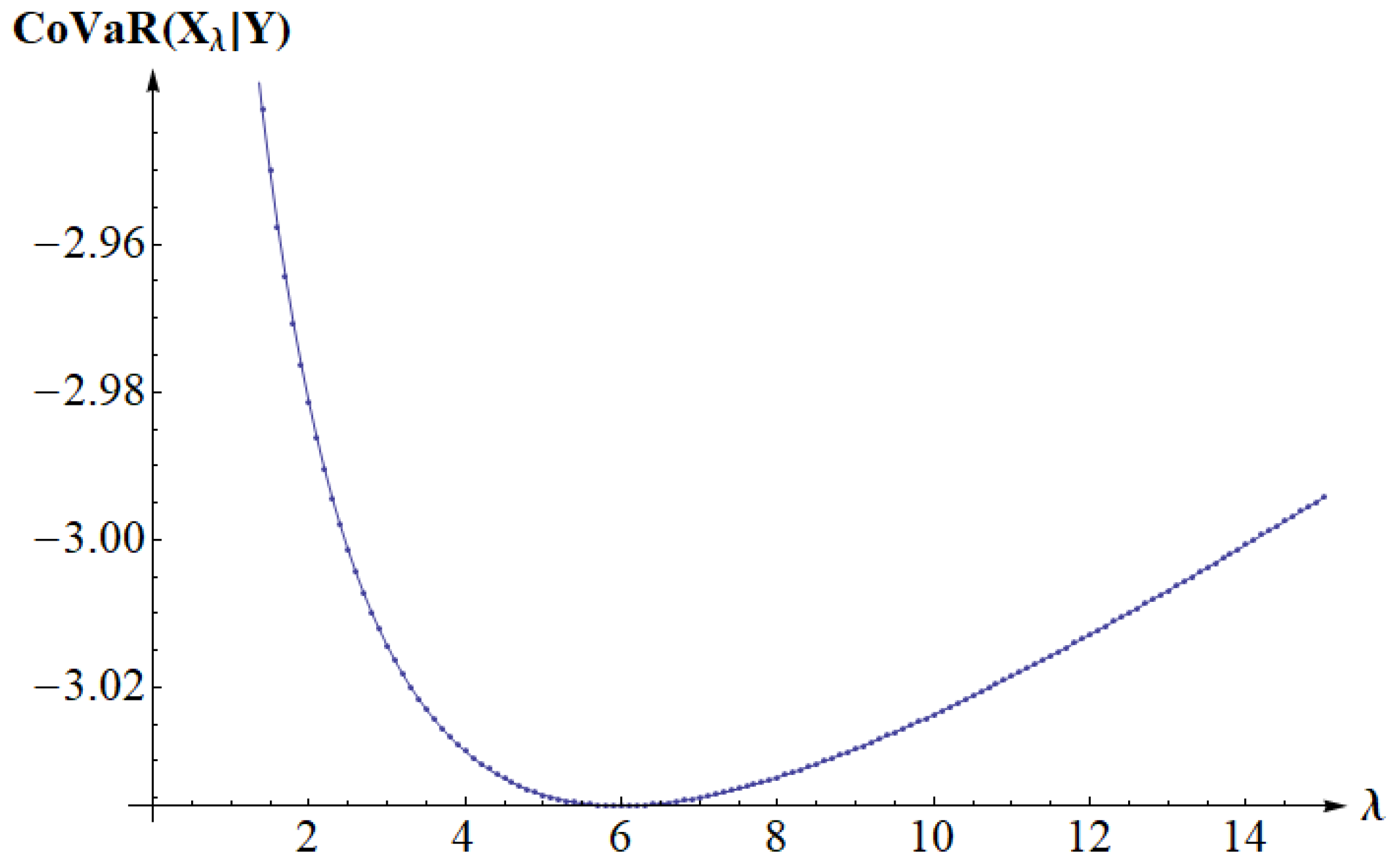
We start with the following basic case:

Lemma 5.

Let ${\left(x_n\right)}_{n=1}^{\infty }$ be a sequence of portfolios fulfilling the constraint ${\mathbb{1}}_n^{\mathrm{T}}x=1$ such that the following hold:

(i). The variance tends to infinity:

$$\underset{n\to \infty }{lim}\left|\right|x_n{\left|\right|}_{\mathsf{\Sigma }}^2=\infty ;$$

(ii). The Sharpe ratio has a limit $s_{*}$:

$$\underset{n\to \infty }{lim}{\displaystyle \frac{{\mu }^T{x}_n}{\left|\right|x_n{\left|\right|}_{\mathsf{\Sigma }}}}=s_{*};$$

(iii). The correlation coefficient with $R_1$ has a limit ${\rho }_{*}$:

$$\underset{n\to \infty }{lim}{cos}_{\mathsf{\Sigma }}(e_1,x_n)={\rho }_{*}.$$

Then,

$$\underset{n\to +\infty }{lim}{CoVaR}_{\alpha ,\beta }^{\le }\left(x_n^{T}R\right|R_1)=\left\{\begin{array}{cc}-\infty & if\beta >{\displaystyle \frac{1}{\alpha }}C\left(\alpha ,\mathsf{\Phi }(-s_{*}),{\rho }_{*}\right),\hfill \\ +\infty & if\beta <{\displaystyle \frac{1}{\alpha }}C\left(\alpha ,\mathsf{\Phi }(-s_{*}),{\rho }_{*}\right).\hfill \end{array}\right.$$

Proof. 

We observe that

$${\displaystyle \frac{{CoVaR}_{\alpha ,\beta }^{\le }\left(x_n^{T}R\right|R_1)}{\left|\right|x_n{\left|\right|}_{\mathsf{\Sigma }}}}=-{\displaystyle \frac{{\mu }^T{x}_n}{\left|\right|x_n{\left|\right|}_{\mathsf{\Sigma }}}}-{\mathsf{\Phi }}^{-1}(w(\alpha ,\beta ,{cos}_{\mathsf{\Sigma }}(e_1,x_n))\stackrel{n\to \infty }{⟶}-s_{*}-{\mathsf{\Phi }}^{-1}\left(w(\alpha ,\beta ,{\rho }_{*})\right).$$

(61)

Since

$$\begin{array}{ccc}\hfill sgn(-s_{*}-{\mathsf{\Phi }}^{-1}\left(w(\alpha ,\beta ,{\rho }_{*})\right)& =& sgn(\mathsf{\Phi }(-s_{*})-w(\alpha ,\beta ,{\rho }_{*}))\hfill \\ & =& sgn(C(\alpha ,\mathsf{\Phi }(-s_{*}),{\rho }_{*})-C(\alpha ,w(\alpha ,\beta ,{\rho }_{*}),{\rho }_{*}))\hfill \\ & =& sgn(C(\alpha ,\mathsf{\Phi }(-s_{*}),{\rho }_{*})-\alpha \beta ),\hfill \end{array}$$

(62)

we obtain for $\beta \ne {\displaystyle \frac{1}{\alpha }}C\left(\alpha ,\mathsf{\Phi }(-s_{*}),{\rho }_{*}\right)$,

$$\underset{n\to +\infty }{lim}{CoVaR}_{\alpha ,\beta }^{\le }\left(x_n^{T}R\right|R_1)=sgn(C(\alpha ,\mathsf{\Phi }(-s_{*}),{\rho }_{*})-\alpha \beta )·\infty .$$

(63)

□

If we add to the assumptions from the above lemma the additional assumption that the sequence $x_n$ belongs to the critical half-plane, then we obtain the dependence between the limiting values $s_{*}$ and ${\rho }_{*}$.

Lemma 6.

Let

$$x_n=X_M\left(E_n\right)-{\lambda }_n{X}_{\infty },E_n,{\lambda }_n>0.$$

Then, the assumptions from Lemma 5 imply that

$$s_{*}^2\le {\displaystyle \frac{1}{\left|\right|X_d{\left|\right|}_{\mathsf{\Sigma }}^2}};$$

and

$${\rho }_{*}=s_{*}\left|\right|X_d{\left|\right|}_{\mathsf{\Sigma }}{cos}_{\mathsf{\Sigma }}(e_1,X_d)-\sqrt{1-s_{*}^2\left|\right|X_d{\left|\right|}_{\mathsf{\Sigma }}^2}{cos}_{\mathsf{\Sigma }}(e_1,X_{\infty }).$$

Proof. 

From the definition of the Sharpe ratio, we obtain

$$s_n={\displaystyle \frac{E_n}{\sqrt{\left|\right|X_M\left(E_n\right){\left|\right|}_{\mathsf{\Sigma }}^2+{\lambda }_n^2\left|\right|X_{\infty }{\left|\right|}^2}}}.$$

Thus,

$${\displaystyle \frac{{\lambda }_n^2}{E_n^2}}\left|\right|X_{\infty }{\left|\right|}^2={\displaystyle \frac{1}{s_n^2}}-{\displaystyle \frac{\left|\right|X_M\left(E\right){\left|\right|}_{\mathsf{\Sigma }}^2}{E^2}}.$$

This implies that the ratio ${\displaystyle \frac{{\lambda }_n}{E_n}}$ has a limit. Based on Formula (45), we obtain

$$\left|\right|X_{\infty }{\left|\right|}^2\underset{n\to \infty }{lim}{\displaystyle \frac{{\lambda }_n^2}{E_n^2}}={\displaystyle \frac{1}{s_{*}^2}}-{\displaystyle \frac{{\gamma }_M}{det\left(G\right)}}.$$

(64)

Obviously, the above implies that

$$s_{*}^2\le {\displaystyle \frac{det\left(G\right)}{{\gamma }_M}}={\displaystyle \frac{1}{\left|\right|X_d{\left|\right|}_{\mathsf{\Sigma }}^2}}.$$

Next,

$$\begin{array}{ccc}\hfill {\rho }_n& =& {cos}_{\mathsf{\Sigma }}(e_1,x_n)={\displaystyle \frac{e_1^T\mathsf{\Sigma }{X}_M\left(E_n\right)-{\lambda }_n{e}_1^T\mathsf{\Sigma }{X}_{\infty }}{\left|\right|e_1{\left|\right|}_{\mathsf{\Sigma }}\left|\right|X_n{\left|\right|}_{\mathsf{\Sigma }}}}\hfill \end{array}$$

(65)

$$\begin{array}{ccc}& =& {\displaystyle \frac{e_1^T\mathsf{\Sigma }{X}_M\left(E_n\right)-{\lambda }_n{e}_1^T\mathsf{\Sigma }{X}_{\infty }}{\left|\right|e_1{\left|\right|}_{\mathsf{\Sigma }}\frac{E_n}{s_n}}}\hfill \end{array}$$

(66)

$$\begin{array}{ccc}& =& {\displaystyle \frac{s_n}{\left|\right|e_1{\left|\right|}_{\mathsf{\Sigma }}}}\left({\displaystyle \frac{e_1^T\mathsf{\Sigma }{X}_M\left(E_n\right)}{E_n}}-{\displaystyle \frac{{\lambda }_n}{E_n}}{e}_1^T\mathsf{\Sigma }{X}_{\infty }\right)\hfill \end{array}$$

(67)

$$\begin{array}{ccc}& \stackrel{n\to \infty }{⟶}& {\displaystyle \frac{s_{*}}{\left|\right|e_1{\left|\right|}_{\mathsf{\Sigma }}}}\left(e_1^T\mathsf{\Sigma }{X}_d-\sqrt{{\displaystyle \frac{1}{s_{*}^2}}-{\displaystyle \frac{{\gamma }_M}{det\left(G\right)}}}{cos}_{\mathsf{\Sigma }}\left(e_1{X}_{\infty }\right)\left|\right|e_1{\left|\right|}_{\mathsf{\Sigma }}\right)\hfill \end{array}$$

(68)

$$\begin{array}{ccc}& =& s_{*}{cos}_{\mathsf{\Sigma }}(e_1,X_d)\left|\right|X_d{\left|\right|}_{\mathsf{\Sigma }}-\sqrt{1-s_{*}^2{\displaystyle \frac{{\gamma }_M}{det\left(G\right)}}}{cos}_{\mathsf{\Sigma }}\left(e_1{X}_{\infty }\right)\hfill \end{array}$$

(69)

$$\begin{array}{ccc}& =& s_{*}\left|\right|X_d{\left|\right|}_{\mathsf{\Sigma }}{cos}_{\mathsf{\Sigma }}(e_1,X_d)-\sqrt{1-s_{*}^2\left|\right|X_d{\left|\right|}_{\mathsf{\Sigma }}^2}{cos}_{\mathsf{\Sigma }}\left(e_1{X}_{\infty }\right).\hfill \end{array}$$

(70)

□

In order to prove point 1 of Theorem 3, we provide for any $\xi \in [0,1]$ such that

$$\beta >{\displaystyle \frac{1}{\alpha }}C\left(\alpha ,{\displaystyle \frac{\xi }{\left|\right|X_d{\left|\right|}_{\mathsf{\Sigma }}}},\xi {cos}_{\mathsf{\Sigma }}(e_1,X_d)-\sqrt{1-{\xi }^2}{cos}_{\mathsf{\Sigma }}(e_1,X_{\infty })\right),$$

a sequence $x_n$ such that

$$\underset{n\to \infty }{lim}{CoVaR}_{\alpha ,\beta }^{\le }(x_n^{T}R,R_1)=-\infty .$$

(71)

We set

$$x_n=X_M\left(n\right)-\sqrt{{\displaystyle \frac{1}{{\xi }^2}}-1}{\displaystyle \frac{\left|\right|X_d{\left|\right|}_{\mathsf{\Sigma }}}{\left|\right|X_{\infty }{\left|\right|}_{\mathsf{\Sigma }}}}n{X}_{\infty }.$$

We obtain

$$\left|\right|x_n{\left|\right|}_{\mathsf{\Sigma }}^2=\left|\right|X_M{\left(n\right)\left|\right|}_{\mathsf{\Sigma }}^2+n^2\left({\displaystyle \frac{1}{{\xi }^2}}-1\right)\left|\right|X_d{\left|\right|}_{\mathsf{\Sigma }}^2,$$

and

$$\begin{array}{ccc}\hfill s_{*}^2& =& \underset{n\to \infty }{lim}{\displaystyle \frac{n^2}{\left|\right|x_n{\left|\right|}_{\mathsf{\Sigma }}^2}}=\underset{n\to \infty }{lim}{\displaystyle \frac{1}{\frac{\left|\right|X_M\left(n\right){\left|\right|}_{\mathsf{\Sigma }}^2}{n^2}+\left(\frac{1}{{\xi }^2}-1\right)\left|\right|X_d{\left|\right|}_{\mathsf{\Sigma }}^2}}\hfill \end{array}$$

(72)

$$\begin{array}{ccc}& =& {\displaystyle \frac{1}{\left|\right|X_d{\left|\right|}_{\mathsf{\Sigma }}+\left(\frac{1}{{\xi }^2}-1\right)\left|\right|X_d{\left|\right|}_{\mathsf{\Sigma }}^2}}={\displaystyle \frac{{\xi }^2}{\left|\right|X_d{\left|\right|}_{\mathsf{\Sigma }}^2}}.\hfill \end{array}$$

(73)

Hence, due to Lemma 6,

$$\begin{array}{ccc}\hfill {\rho }_{*}& =& s_{*}\sqrt{{\displaystyle \frac{{\gamma }_M}{det\left(G\right)}}}{cos}_{\mathsf{\Sigma }}(e_1,X_d)-\sqrt{1-s_{*}^2{\displaystyle \frac{{\gamma }_M}{det\left(G\right)}}}{cos}_{\mathsf{\Sigma }}(e_1,X_{\infty })\hfill \\ & =& \xi {cos}_{\mathsf{\Sigma }}(e_1,X_d)-\sqrt{1-{\xi }^2}{cos}_{\mathsf{\Sigma }}(e_1,X_{\infty })\hfill \end{array}$$

(74)

Finally, Lemma 5 implies that the limit from (71) equals $-\infty$.

Next, we prove point 2 of Theorem 3. We assume that

$$\beta <min\left({\displaystyle \frac{1}{\alpha }}C\left(\alpha ,\mathsf{\Phi }\left({\displaystyle \frac{-\xi }{\left|\right|X_d{\left|\right|}_{\mathsf{\Sigma }}}}\right),\xi {cos}_{\mathsf{\Sigma }}(e_1,X_d)-\sqrt{1-{\xi }^2}{cos}_{\mathsf{\Sigma }}(e_1,X_{\infty })\right)|\xi \in [0,1]\right).$$

(75)

We denote by $in{f}_{*}$ the infimum of the ${CoVaR}_{\alpha ,\beta }^{\le }$:

$$\begin{array}{ccc}\hfill in{f}_{*}& =& inf\left\{{CoVaR}_{\alpha ,\beta }(x^{T}R,R_1)\right|x^{\mathrm{T}}{\mathbb{1}}_n=1\}\hfill \\ & =& inf(-x^T\mu -{\mathsf{\Phi }}^{-1}(w(\alpha ,\beta ,{cos}_{\mathsf{\Sigma }}(e_1,x)){\left|\right|x\left|\right|}_{\mathsf{\Sigma }}|x^{\mathrm{T}}{\mathbb{1}}_n=1).\hfill \end{array}$$

(76)

Let the sequence ${\left(x_n\right)}_1^{\infty }$ be a sequence of portfolios approaching $in{f}_{*}$:

$$x_n^T{\mathbb{1}}_n=1,\underset{n\to \infty }{lim}(-x_n^T\mu -{\mathsf{\Phi }}^{-1}(w(\alpha ,\beta ,{cos}_{\mathsf{\Sigma }}(e_1,x_n))\left|\right|x_n{\left|\right|}_{\mathsf{\Sigma }})=in{f}_{*}.$$

We show that the assumption (75) implies that the sequence $x_n$ must be bounded. Indeed, there would otherwise exist a subsequence $x_{n_k}$ such that

$$\left|\right|x_{n_k}{\left|\right|}_{\mathsf{\Sigma }}⟶+\infty .$$

Since the Sharpe ratio

$$s_{n_k}={\displaystyle \frac{x_{n_k}^T\mu }{\left|\right|x_{n_k}{\left|\right|}_{\mathsf{\Sigma }}}}$$

and correlation coefficient

$${cos}_{\mathsf{\Sigma }}(e_1,x_n)={\displaystyle \frac{e_1^T\mathsf{\Sigma }{x}_n}{\left|\right|e_1{\left|\right|}_{\mathsf{\Sigma }}\left|\right|x_n{\left|\right|}_{\mathsf{\Sigma }}}}$$

belong to a bounded sets (see Lemma 2), we might select the subsequence $x_{n_k}$ in such a way that these ratios and coefficients have limits. We denote these limits by $s_{*}$ and ${\rho }_{*}$:

$$\begin{array}{ccc}\hfill s_{*}& =& \underset{k\to \infty }{lim}{\displaystyle \frac{x_{n_k}^T\mu }{\left|\right|x_{n_k}{\left|\right|}_{\mathsf{\Sigma }}}},\hfill \end{array}$$

(77)

$$\begin{array}{ccc}\hfill {\rho }_{*}& =& \underset{k\to \infty }{lim}{cos}_{\mathsf{\Sigma }}(e_1,x_{n_k})\hfill \end{array}$$

(78)

Due to Lemma 3 ($t=\left|\right|x_{n_k}{\left|\right|}_{\mathsf{\Sigma }}$, $E=x_{n_k}^T\mu$) and Lemma 6,

$$\begin{array}{ccc}\hfill {\rho }_{*}& =& \underset{k\to \infty }{lim}{cos}_{\mathsf{\Sigma }}(e_1,x_{n_k})\ge \underset{k\to \infty }{lim}{cos}_{\mathsf{\Sigma }}(e_1,X_M\left(x_{n_k}^T\mu \right)-{\lambda }_k{X}_{\infty })\hfill \\ & =& s_{*}\left|\right|X_d{\left|\right|}_{\mathsf{\Sigma }}{cos}_{\mathsf{\Sigma }}(e_1,X_d)-\sqrt{1-s_{*}^2\left|\right|X_d{\left|\right|}_{\mathsf{\Sigma }}^2}{cos}_{\mathsf{\Sigma }}(e_1,X_{\infty }).\hfill \end{array}$$

(79)

Thus, assumption (75) and Lemma 5 imply that

$$\underset{k\to \infty }{lim}{CoVaR}_{\alpha ,\beta }^{\le }(x_{n_k}^{T}R,R_1)=+\infty .$$

(80)

which contradicts the assumption that the sequence $x_n$ is approaching the infimum of CoVaR.

5. Examples

We consider the following data:

$$\mathsf{\Sigma }=\left(\begin{array}{cccc}1& {\displaystyle \frac{1}{5}}& 1& -1\\ {\displaystyle \frac{1}{5}}& 1& 0& -1\\ 1& 0& 9& 0\\ -1& -1& 0& 4\end{array}\right)\mathrm{and}\mu =\left(\begin{array}{c}2\\ 3\\ 1\\ 3\end{array}\right)$$

We obtain

$$det\left(\mathsf{\Sigma }\right)=17.16,$$

$$G={\displaystyle \frac{1}{17.16}}\left(\begin{array}{cc}587.6& 217.36\\ 217.36& 82.28\end{array}\right).$$

$$X_M{\left(E\right)}^T={\displaystyle \frac{1}{64.24}}\left((142,-98,25.36,-5.12)+E(-44,46.2,-10.12,7.92)\right),$$

$$X_{\infty }^T={\displaystyle \frac{1}{64.24}}(10.24,5.6,-5.12,-10.72).$$

Finally,

$${cos}_{\mathsf{\Sigma }}(e_1,X_{\infty })=2\sqrt{{\displaystyle \frac{53}{803}}}.$$

We fix E and study the half-line of the portfolios:

$$X_{\lambda }=X_M\left(E\right)-\lambda X_{\infty },\lambda \ge 0.$$

Example 1.

We have ${\rho }_{\infty }=-{cos}_{\mathsf{\Sigma }}(e_1,X_{\infty })=-2\sqrt{{\displaystyle \frac{53}{803}}}$. We choose

$$\alpha =\mathsf{\Phi }\left(-{\displaystyle \frac{3}{5}}\right),\beta ={\displaystyle \frac{{\mathsf{\Phi }}_2\left(-\frac{3}{5},0;{\rho }_{\infty }\right)}{\mathsf{\Phi }\left(-\frac{3}{5}\right)}},E={\displaystyle \frac{637}{220}}.$$

This way, we obtain

$$\beta ={\displaystyle \frac{1}{\alpha }}C\left(\alpha ,{\displaystyle \frac{1}{2}},-{cos}_{\mathsf{\Sigma }}(e_1,X_{\infty })\right),{\mathsf{\Phi }}^{-1}\left(w\left({\rho }_{\infty }\right)\right)=0, and{cos}_{\mathsf{\Sigma }}(X_M,e_1)=0.$$

Therefore,

$${CoVaR}_{\alpha ,\beta }^{\le }(X_{\lambda }\mid Y)=-{\displaystyle \frac{637}{220}}-{\mathsf{\Phi }}^{-1}\left(w\left(\rho \left(\lambda \right)\right)\right)\sqrt{{\displaystyle \frac{212{\lambda }^2}{803}}+{\displaystyle \frac{2561}{8800}}}$$

where

$$\rho \left(\lambda \right)={cos}_{\mathsf{\Sigma }}(X_{\lambda },e_1)={\displaystyle \frac{-212\lambda }{803\sqrt{\frac{212{\lambda }^2}{803}+\frac{2561}{8800}}}}>{\rho }_{\infty },$$

for any $\lambda >0$ and in consequence $-{\mathsf{\Phi }}^{-1}\left(w\left(\rho \left(\lambda \right)\right)\right)>0$. From Lemma 4, we have

$$\begin{array}{c}\hfill \underset{\lambda \to \infty }{lim}CoVaR\left(X_{\lambda }\right|Y)=-{\displaystyle \frac{637}{220}}<{CoVaR}_{\alpha ,\beta }^{\le }(X_{\lambda }\mid Y)\end{array}$$

Thus, the global minimum cannot exist. We illustrate this in Figure 3.

Example 2.

We consider the same data. However, we now choose

$$\alpha =\mathsf{\Phi }\left(-{\displaystyle \frac{3}{5}}\right),\beta ={\displaystyle \frac{{\mathsf{\Phi }}_2\left(-\frac{3}{5},0;{\rho }_{\infty }-\frac{1}{100}\right)}{\mathsf{\Phi }\left(-\frac{3}{5}\right)}}.$$

This way, we obtain $\beta <{\displaystyle \frac{1}{\alpha }}C\left(\alpha ,{\displaystyle \frac{1}{2}},-{cos}_{\mathsf{\Sigma }}(e_1,X_{\infty })\right)$, and the optimization problem has a solution. We have

$${CoVaR}_{\alpha ,\beta }^{\le }(X\mid Y)=-E-{\mathsf{\Phi }}^{-1}\left(w\left(\rho \left(\lambda \right)\right)\right)\sqrt{{\displaystyle \frac{2057E^2-10868E+424{\lambda }^2+14690}{1606}}}$$

where $\rho \left(\lambda \right)={\displaystyle \frac{\sqrt{2}(-660E-212\lambda +1911)}{\sqrt{803\left(2057E^2-10868E+424{\lambda }^2+14690\right)}}}$. We approximate ${\mathsf{\Phi }}^{-1}\left(w\left(\rho \left(\lambda \right)\right)\right)$ numerically based on formulas (32) and (37). We solve numerically the differential equation

$${\displaystyle \frac{dY}{d\lambda }}=-{\displaystyle \frac{\frac{1}{\sqrt{2\pi (1-\rho {\left(\lambda \right)}^2)}}exp\left(-\frac{{({\mathsf{\Phi }}^{-1}\left(\alpha \right)-\rho \left(\lambda \right)Y)}^2}{2(1-\rho {\left(\lambda \right)}^2)}\right)}{\mathsf{\Phi }\left(\frac{{\mathsf{\Phi }}^{-1}\left(\alpha \right)-\rho \left(\lambda \right)Y}{\sqrt{1-\rho {\left(\lambda \right)}^2}}\right)}}{\rho }^{\prime }\left(\lambda \right),$$

with initial value $Y\left({\lambda }_0\right)={\mathsf{\Phi }}^{-1}\left(\beta \right)$, with ${\lambda }_0={\displaystyle \frac{1911-660E}{212}}$. We find ${\lambda }_1$ such that for $\lambda >{\lambda }_1,$${CoVaR}_{\alpha ,\beta }^{\le }$ is increasing. Next, we use Wolfram Mathematica to numerically minimize ${CoVaR}_{\alpha ,\beta }^{\le }$ along the line segment $[0,{\lambda }_1]$.

For $E=2$, we have $\rho (x_M,e_1)>0$. We thus obtain the numerically calculated minimum $-0.815187\dots$ for $\lambda =4.211162\dots$ as illustrated at Figure 4.

For $E=-1$, we have ${CoVaR}_{\alpha ,\beta }^{\le }{|}_{\lambda =0}>0$. We obtain the numerically calculated minimum $6.254844\dots$ for $\lambda =24.788285\dots$ as illustrated at Figure 5. As the reader can guess, it is easier to subtract a certain constant from CoVaR to show that the new function is positive for $\lambda >210$.

For $E={\displaystyle \frac{637}{220}}$, we have $\rho (x_M,e_1)=0$. We obtain the numerically calculated minimum $-2.812375\dots$ for $\lambda =5.271369\dots$ as illustrated at Figure 6.

For $E=3$, we obtain $\rho (x_M,e_1)<0$. We thus obtain the numerically calculated minimum $-3.036088\dots$ for $\lambda =5.991312\dots$ as illustrated at Figure 7.

All the numerical calculations seem to point to the existence of a unique solution under the conditions of Theorem 3.

6. Conclusions

Contrary to the standard ${CoVaR}_{\mathrm{ff},\mathrm{fi}}^{=}$, our modified version, ${CoVaR}_{\alpha ,\beta }^{\le }$, does not provide us with an easy analytical formula for calculating the minimal-risk-for-fixed-return portfolio, challenging us to account for the numerically found solutions that, judging from the data, could even be unique and perhaps a global minimum of an elusively convex function. We have shown in Theorem 2 that there is a curve dividing ${(0,1)}^2$ sets of possible significance levels $\alpha$ and $\beta$ into two sets: one in which our optimization problem has a solution, and one in which it does not. We also noticed that for $\alpha$ and $\beta$ belonging to the curve of division, the infimum of ${CoVaR}_{\alpha ,\beta }^{\le }$ is finite but the optimal portfolio may not exist. Thus, there are still open questions in this Gaussian setting. The next step would be to widen our scope to all elliptical distributions.

References

1. Alexander, G.J.; Francis, J.C. Portfolio Analysis, 3rd ed.; Prentice-Hall: New Jersey, NJ, USA, 1986. [Google Scholar]
2. Black, F. Capital market equilibrium with restricted borrowing. J. Bus. 1972, 45, 444–455. [Google Scholar] [CrossRef]
3. Tobin, J. Liquidity preference as behavior towards risk. Rev. Econ. Stud. 1958, 25, 65–86. [Google Scholar] [CrossRef]
4. Frost, P.A.; Savarino, J.E. An Empirical Bayes Approach to Efficient Portfolio Selection. J. Financ. Quant. Anal. 1986, 3, 293–305. [Google Scholar] [CrossRef]
5. Frost, P.A.; Savarino, J.E. For better performance: Constrain portfolio weights. J. Portf. Manag. 1988, 15, 29. [Google Scholar] [CrossRef]
6. Petukhina, A.; Klochkov, Y.; Härdle, W.K.; Zhivotovskiy, N. Robustifying Markowitz. J. Econom. 2024, 239, 105387. [Google Scholar] [CrossRef]
7. Black, F.; Litterman, R. Global Portfolio Optimization. Financ. Anal. J. 1922, 48, 28–43. [Google Scholar] [CrossRef]
8. Idzorek, T. A step-by-step guide to the Black-Litterman model: Incorporating user-specified confidence levels. In Forecasting Expected Returns in the Financial Markets; Elsevier: Amsterdam, The Netherlands, 2007; pp. 17–38. [Google Scholar]
9. Palczewski, A.; Palczewski, J. Black–Litterman model for continuous distributions. Eur. J. Oper. Res. 2019, 273, 708–720. [Google Scholar] [CrossRef]
10. Jagannathan, R.; Tongshu, M. Risk reduction in large portfolios: Why imposing the wrong constraints helps. J. Financ. 2003, 58, 1651–1683. [Google Scholar] [CrossRef]
11. Adrian, T.; Brunnermeier, M.K. CoVaR (Working Paper 17454); National Bureau of Economic Research Working Paper Series; National Bureau of Economic Research: Cambridge, MA, USA, 2011. [Google Scholar]
12. Adrian, T.; Brunnermeier, M.K. CoVaR. Am. Econ. Rev. 2016, 106, 1705–1741. [Google Scholar] [CrossRef]
13. Bernardi, M.; Durante, F.; Jaworski, P. Covar of families of copulas. Stat. Probab. Lett. 2017, 120, 8–17. [Google Scholar] [CrossRef]
14. Föllmer, H.; Schied, A. Stochastic Finance. An Introduction in Discrete Time, 2nd ed.; de Gruyter: Berlin, Germany, 2004. [Google Scholar]
15. Jaworski, P. On the Conditional Value at Risk (CoVaR) for tail-dependent copulas. Depend. Model. 2017, 5, 1–15. [Google Scholar] [CrossRef]
16. Jaworski, P. On the Conditional Value-at-Risk (CoVaR) in copula setting. In Copulas and Dependence Models with Applications; Úbeda Flores, M., de Amo Artero, E., Durante, F., Fernández-Sánchez, J., Eds.; Springer: Cham, Switzerland, 2017; pp. 95–117. [Google Scholar]
17. Zalewska, A. On peculiarities of covar-based portfolio selection. Appl. Math. 2018, 45, 181–197. [Google Scholar]
18. Bernardi, M.; Durante, F.; Jaworski, P.; Petrella, L.; Salvadori, G. Conditional Risk based on multivariate Hazard Scenarios. Stoch. Environ. Res. Risk Assess. 2018, 32, 203–211. [Google Scholar] [CrossRef]
19. Hakwa, B.; Jäger-Ambrozewicz, M.; Rüdiger, B. Analysing systemic risk contribution using a closed formula for conditional Value at Risk through copula. Commun. Stoch. Anal. 2015, 9, 131–158. [Google Scholar] [CrossRef]
20. Mainik, G.; Schaanning, E. On dependence consistency of CoVaR and some other systemic risk measures. Stat. Risk Model. 2014, 31, 49–77. [Google Scholar] [CrossRef]
21. Girardi, G.; Ergün, T.A. Systemic risk measurement: Multivariate GARCH estimation of CoVar. J. Bank. Financ. 2013, 37, 3169–3180. [Google Scholar] [CrossRef]
22. Nelsen, R.B. An Introduction to Copulas, 2nd ed.; Springer Series in Statistics; Springer: New York, NY, USA, 2006. [Google Scholar]
23. Cherubini, U.; Luciano, E.; Vecchiato, W. Copula Methods in Finance; John Wiley & Sons Ltd.: Hoboken, NJ, USA, 2004. [Google Scholar]
24. Durante, F.; Sempi, C. Principles of Copula Theory; CRC Press: Boca Raton, FL, USA, 2016. [Google Scholar]
25. Embrechts, P. Copulas: A personal view. J. Risk Insur. 2009, 76, 639–650. [Google Scholar] [CrossRef]
26. Joe, H. Dependence Modeling with Copulas; Chapman & Hall/CRC: London, UK, 2014. [Google Scholar]
27. McNeil, A.J.; Frey, R.; Embrechts, P. Quantitative Risk Management. Concepts, Techniques and Tools; Princeton Series in Finance; Princeton University Press: Princeton, NJ, USA, 2005. [Google Scholar]
28. Mai, J.; Scherer, M. Simulating Copulas: Stochastic Models, Sampling Algorithms, and Applications; Series in Quantitative Finance; Imperial College Press: London, UK, 2012. [Google Scholar]
29. Meyer, C. The bivariate normal copula. Commun. Stat. Theory Methods 2013, 42, 2402–2422. [Google Scholar] [CrossRef]
30. Sheppard, W.F. On the calculation of the double integral expressing normal correlation. Trans. Camb. Phil. Soc. 1900, 19, 23–68. [Google Scholar]
Figure 1. Horizontal sections of a chosen Gaussian copula.
Mathematics 12 03766 g001
Figure 2. Graph of function ρ Φ 1 ( w ( 0.05 , 0.01 , ρ ) ) .
Mathematics 12 03766 g002
Figure 3. Numerically calculated CoVaR as function of λ .
Mathematics 12 03766 g003
Figure 4. Numerically calculated CoVaR for E = 2 .
Mathematics 12 03766 g004
Figure 5. Numerically calculated CoVaR 7.5 for E = 1 .
Mathematics 12 03766 g005
Figure 6. Numerically calculated CoVaR for E = 637 220 .
Mathematics 12 03766 g006
Figure 7. Numerically calculated CoVaR for E = 3 .
Mathematics 12 03766 g007
Disclaimer/Publisher’s Note: The statements, opinions and data contained in all publications are solely those of the individual author(s) and contributor(s) and not of MDPI and/or the editor(s). MDPI and/or the editor(s) disclaim responsibility for any injury to people or property resulting from any ideas, methods, instructions or products referred to in the content.