An Adapted Proximal Point Algorithm Utilizing the Golden Ratio Technique for Solving Equilibrium Problems in Banach Spaces

Abstract

This paper explores the iterative approximation of solutions to equilibrium problems and proposes a simple proximal point method for addressing them. We incorporate the golden ratio technique as an extrapolation method, resulting in a two-step iterative process. This method is self-adaptive and does not require any Lipschitz-type conditions for implementation. We present and prove a weak convergence theorem along with a sublinear convergence rate for our method. The results extend some previously published findings from Hilbert spaces to 2-uniformly convex Banach spaces. To demonstrate the effectiveness of the method, we provide several numerical illustrations and compare the results with those from other methods available in the literature.

1. Introduction

In this paper, we focus on studying an iterative approximation of the Equilibrium Problem (EP), which is defined by the following condition:

$$\mathrm{Find}{s}^{*}\in \mathcal{K}\mathrm{such}\mathrm{that}f(s^{*},s)\ge 0,\forall s\in \mathcal{K},$$

where $f:\mathcal{K}\times \mathcal{K}\to \mathbb{R}$ is a bifunction, and $\mathcal{K}\ne \varnothing$ is a closed and convex subset of a real Banach space E. We denote the solution set of the EP by $\Omega$ whenever the problem is consistent. The introduction of the EP is attributed to Blum and Oettli [1], with additional contributions from [2] in the early 1990s. Both of these works are based on the minimax inequality considered by Ky Fan [3]. As presented in this form, the EP serves as a unified framework for studying several optimization and fixed-point problems, including variational inequalities, complementarity problems, saddle point problems, and Nash equilibrium problems, among others.

In recent years, the EP has attracted significant interest from various researchers, leading to the development of several prominent solution methods. Notable among these are gap function methods [4], auxiliary problem principle methods [5], and proximal point methods [2,6]. The proximal method, in particular, has garnered considerable attention as a means of obtaining approximate solutions to the EP [6,7]. This method is based on the auxiliary problem principle initially introduced by Cohen [8] and later adapted to the EP in real Banach space by Mastroeni [5]. It is important to note that the proximal method is particularly effective when the bifunction is strongly monotone or monotone. In 2008, Tran et al. [9] extended the proximal point method for solving the equilibrium problem (EP) under the assumption that the bifunction is pseudomonotone and satisfies a Lipschitz-type condition. This proposed method, also known as the extragradient method, is a two-step proximal point method that builds on Korpelevich’s extragradient method (see [10]) within the EP framework.

It is worth mentioning that the construction of the extragradient method by Tran et al. [9] requires satisfying a Lipschitz-type condition, particularly regarding the selection of the scaling parameter $\alpha$, which must fall in the range of $\left(0,min\{{\displaystyle \frac{1}{2c_1}},{\displaystyle \frac{1}{2c_2}}\}\right)$, where $c_1$ and $c_2$ are the Lipschitz-type constants of the bifunction. Since then, numerous extensions and modifications of this method have emerged in various directions (see [11,12,13,14,15,16]).

Hieu [13], drawing from the subgradient technique developed by Censor et al. [17,18], introduced a subgradient extragradient method to solve the EP associated with a pseudomonotone operator. In this approach, the second optimization subproblem is altered by replacing the feasible set with a constructible half-space. Similar to the method proposed by Tran et al. [9], Hieu’s method [13] also relies on knowledge of the Lipschitz condition of the cost function. In the context of 2-uniformly convex Banach spaces, Ogbuisi [19] proposed a Popov subgradient extragradient method for approximating solutions to the equilibrium problem (EP). He established a weak convergence theorem under the condition that the scaling parameter satisfies specific requirements related to Lipschitz-type constants $c_1$ and $c_2$. However, the reliance of these methods on the Lipschitz constant poses significant limitations, especially due to the nonlinear nature of the function, thus restricting the applicability of these methods.

To address this limitation, Yang and Liu [15,16] introduced a self-adaptive subgradient extragradient method. In their approach, the scaling parameter is updated using a formula that begins with a known initial point, thereby enhancing the scope of the subgradient extragradient method. Jolaoso and Aphane [20] proposed two subgradient extragradient methods for solving the EP. The first method, similar to Ogbuisi’s, relies on the Lipschitz-type condition. However, in their second method, they utilized the self-adaptive technique, extending the work of Yang and Liu [15,16] to the framework of 2-uniformly convex Banach spaces. It is important to note that both the extragradient method and its subgradient versions require solving a strongly convex optimization problem twice per iteration, which can be time-consuming and memory-intensive.

Recently, Hoai [21] introduced a modified proximal point algorithm based on the golden ratio technique within the framework of a real Hilbert space. A noteworthy feature of this method is that it requires solving only one strongly convex optimization problem per iteration. This improvement over the original proximal point method is attributed to the incorporation of the golden ratio. The golden ratio method was initially proposed by Malitsky [22] for solving Mixed Variational Inequalities, and it has recently been studied as an extrapolation technique to enhance the convergence properties of iterative algorithms (see [22,23]) and the references therein. To generate a sequence $\left\{s_n\right\}$ using this method, an extra step $r_n$, which is a weighted average of the current $s_n$ and the previous $r_{n-1}$ scaled by $\varphi ={\displaystyle \frac{\sqrt{5}+1}{2}}$, is introduced. Due to the improvements observed in the convergence properties of iterative methods, researchers have increasingly considered the application of this technique (see [21,24,25,26]).

Building upon the works of Hoai [21], Ogbuisi [19], and Jolaoso [20], we introduced a simple proximal point method based on the golden ratio technique for solving the EP in the context of 2-uniformly convex Banach spaces. This method, which combines proximal point and golden ratio approaches, is self-adaptive and eliminates the need for prior knowledge of the Lipschitz-type constants of the associated pseudomonotone operator. Using the proposed method, we establish and prove a weak convergence theorem, along with a sublinear rate of convergence for the method.

The manuscript is structured as follows: In Section 2, we review important definitions and results, and we derive analogs of two well-known results from Hilbert spaces. The main result is presented in Section 3, which begins with key assumptions and an introduction to the methodology. Section 4 contains numerical illustrations that demonstrate the performance of the method, along with comparisons to previously published results. Finally, we conclude the manuscript with a summary in the last section.

2. Preliminary Results

In this section, we revisit several foundational definitions and relevant lemmas. Let $\mathcal{K}\ne \varnothing$ be a closed and convex subset of a real Banach space E with norm $\parallel ·\parallel$. We denote the dual space of E as $E^{*}$ and the duality pairing between elements of E and $E^{*}$ as $⟨·,·⟩$. The weak convergence of a sequence $\left\{s_n\right\}$ to a point $s^{*}\in E$ is expressed as $s_n\rightharpoonup s^{*}$.

Let $J:E\to 2^{E^{*}}$ be the normalized duality mapping defined by

$$Jx=\{s^{*}\in E^{*}:⟨s,s^{*}⟩=\parallel s\parallel =\parallel s^{*}{\parallel }^2,\forall s\in E\}.$$

We also define the Lyapunov functional $\varphi :E\times E\to {\mathbb{R}}_{+}$ as follows (see [27]):

$$\varphi (s,t)={\parallel s\parallel }^2-2⟨s,Jt⟩+{\parallel t\parallel }^2,\forall s,t\in E.$$

From the definition of $\varphi$, it is evident that

$${\left(\parallel s\parallel -\parallel t\parallel \right)}^2\le \varphi (s,t)\le {\left(\parallel s\parallel +\parallel t\parallel \right)}^2.$$

We will also require the following property of the functional $\varphi$ (see [28,29]):

$$\begin{array}{c}\hfill \varphi (s,u)=\varphi (s,t)+\varphi (t,u)+2⟨s-t,Jt-Ju⟩.\end{array}$$

(1)

Also in [27], Alber introduced the generalized projection operator defined by

$${\Pi }_{\mathcal{K}}s=\underset{t\in \mathcal{K}}{inf}\{\varphi (t,s),\forall s\in E\}.$$

The generalized projection operator satisfies the following property as given in the next result.

Lemma 1

([27]). Let $\mathcal{K}\ne \varnothing$ be a closed and convex subset of a smooth, strictly convex, and reflexive real Banach space $E.$ If $s\in E$ and $t\in \mathcal{K},$ then

$$t={\Pi }_{\mathcal{K}}s\iff ⟨u-t,Js-Jt⟩\le 0,\forall u\in \mathcal{K}$$

and

$$\varphi (u,{\Pi }_{\mathcal{K}}s)+\varphi ({\Pi }_{\mathcal{K}}s,s)\le \varphi (u,s),\forall u\in \mathcal{K},s\in E.$$

In the case where $E=H$ is a real Hilbert space, then $\varphi (s,t)={\parallel s-t\parallel }^2$ and ${\Pi }_{\mathcal{K}}$ reduces to the metric projection (see [30]).

Definition 1.

Let $\mathcal{K}\ne \varnothing$ be a closed and convex subset of E and let $f:\mathcal{K}\times \mathcal{K}\to \mathbb{R}$ be a bifunction. Then, f is

(1) 

strongly monotone, if there exists a positive constant γ, such that

$${f(s,t)+f(t,s)+\gamma \parallel s-t\parallel }^2\le 0,\forall s,t\in \mathcal{K};$$

(2) 

monotone, if

$$f(s,t)+f(t,s)\le 0,\forall s,t\in \mathcal{K};$$

(3) 

strongly pseudomonotone, if there exists a positive constant γ, such that

$$f(s,t)\ge 0\Rightarrow {f(t,s)+\gamma \parallel s-t\parallel }^2\le 0,\forall s,t\in \mathcal{K};$$

(4) 

pseudomonotone, if

$$f(s,t)\ge 0\Rightarrow f(t,s)\le 0,\forall s,t\in \mathcal{K};$$

(5) 

(see Theorem 3.1(v), [4]). Lipschitz-type on $\mathcal{K}$ if there exists a positive constant $L>0$

$$f(p,r)-f(p,q)-f(q,r)\le L\parallel p-q\parallel \parallel q-r\parallel ,\forall p,q,r\in \mathcal{K}.$$

We note that the above inequality corresponds to

$$\begin{array}{c}\hfill f(p,r)-f(p,q)-f(q,r)\le c_1{\parallel p-q\parallel }^2+c_2{\parallel q-r\parallel }^2,\forall p,q,r\in \mathcal{K},\end{array}$$

(2)

where $2c_1=2c_2=L.$

• Clearly $\left(1\right)\Rightarrow \left(2\right)\Rightarrow \left(4\right).$

Denote the unit sphere and unit ball of a real Banach space E by $S_E$ and $B_E$, repectively. The modulus of convexity of E is the function ${\delta }_E:(0,2]\to [0,1]$ defined by

$$\begin{array}{c}\hfill {\delta }_E\left(ϵ\right)=inf\left\{1-{\displaystyle \frac{1}{2}}\parallel s+t\parallel :s,t\in B_E,\parallel s-t\parallel \ge ϵ\right\}.\end{array}$$

A Banach space E is said to be uniformly convex if ${\delta }_E\left(ϵ\right)>0$ for any $(0,2]$ and 2-uniformly convex if there exists a constant $\kappa >0$, such that ${\delta }_E\left(ϵ\right)>\kappa {ϵ}^2$ for any $ϵ\in (0,2].$ It is obvious that every 2-uniformly convex Banach space is uniformly convex. The Banach space E is said to be strictly convex if $\parallel s+t\parallel <2$ for every $s,t\in S_E$ with $s\ne t.$ The modulus of smoothness of E is the function ${\rho }_E:[0,+\infty )\to [0,+\infty )$ defined by

$$\begin{array}{c}\hfill {\rho }_E\left(\lambda \right)=sup\left\{{\displaystyle \frac{1}{2}}(\parallel s+\lambda t\parallel -\parallel s-\lambda t\parallel )-1:s\in S_E,\parallel t\parallel \le \lambda \right\}.\end{array}$$

The Banach space E is said to be uniformly smooth if $\underset{\lambda \to 0}{lim}{\displaystyle \frac{{\rho }_E\left(\lambda \right)}{\lambda }}=0$ and 2-uniformly smooth if there exists a constant $c>0$, such that ${\rho }_E\left(\lambda \right)<c{\lambda }^2.$ Also, E is said to be smooth if the limit

$$\underset{\lambda \to 0}{lim}{\displaystyle \frac{\parallel s+\lambda t\parallel -\parallel s\parallel }{\lambda }}$$

exists for all $s,t\in S_E.$ It is well known that every 2-uniformly smooth Banach space is uniformly smooth. See [30,31] for more on the geometry of Banach spaces.

Lemma 2

([32]). Let E be a smooth and uniformly convex real Banach space, let $\left\{x_n\right\}$ and $\left\{y_n\right\}$ be sequences in $E.$ If either $\left\{x_n\right\}$ or $\left\{y_n\right\}$ is bounded and $\varphi (x_n,y_n)\to 0$ as $n\to \infty ,$ then $\parallel x_n-y_n\parallel \to 0$ as $n\to \infty .$

Lemma 3

([33]). Let E be a 2-uniformly convex Banach space. Then, there exists a constant $\kappa >0$, such that

$${\kappa \parallel x-y\parallel }^2\le \varphi (x,y),\forall x,y\in E.$$

Lemma 4

([34]). Let ${\displaystyle \frac{1}{p}}+{\displaystyle \frac{1}{q}}=1,p,q>1.$ The space E is q-uniformly smooth if and only if its dual $E^{*}$ is p-uniformly convex.

We use the following definitions in the sequel. The normal cone $N_{\mathcal{K}}$ to a set $\mathcal{K}$ at a point $t\in \mathcal{K}$ is given by

$$N_{\mathcal{K}}\left(s\right)=\{s^{*}\in E^{*}:⟨s-t,s^{*}⟩\ge 0,\forall t\in \mathcal{K}\}.$$

Let $h:\mathcal{K}\to \mathbb{R}$ be a function. The subdifferential of h at s is defined by

$$\partial h\left(s\right)=\{s^{*}\in E^{*}:h\left(t\right)-h\left(s\right)\ge ⟨s^{*},t-s⟩,\forall t\in \mathcal{K}.\}$$

Remark 1.

Observe from the definitions of the subdifferential and $\varphi (s,t),$ that

$$\partial \varphi (·,t)\left(s\right)=\left\{2\right(Js-Jt\left)\right\}.$$

Lemma 5

(Chapter 7, Section 7.2, [35]). Let $\mathcal{K}\ne \varnothing$ be convex subset of a Banach space E and $h:\mathcal{K}\to \mathbb{R}\cup \{+\infty \}$ be a convex, subdifferentiable and lower semicontinuous function. Furthermore, the function h satisfies the following regularity condition:

$$Eitherint\left(\mathcal{K}\right)\ne \varnothing orgis continuous at a point in\mathcal{K}.$$

Then, $s^{*}$ is a solution to the following convex optimization problem

$$\underset{s\in \mathcal{K}}{min}h\left(s\right)$$

if and only if $0\in \partial h\left(s^{*}\right)+N_{\mathcal{K}}\left(s^{*}\right).$

Let $\mathcal{K}\ne \varnothing$ be a closed and convex subset of a real Banach space $E,$ $h:\mathcal{K}\to \mathbb{R}$ be a convex function. Let $\alpha >0$ be a scaling parameter. The proximal mapping of h is defined by

$$pro{x}_{\alpha h}\left(s\right)=arg\underset{t\in \mathcal{K}}{min}\left\{\alpha h\left(t\right)+{\displaystyle \frac{1}{2}}\varphi (s,t)\right\},\forall s\in E.$$

Remark 2.

From (Chapter 3, Section 3.2, [36]) it is known that $pro{x}_{\alpha h}\left(s\right)$ is single-valued. By the definition of $\partial h\left(pro{x}_{\alpha h}\left(s\right)\right)$ and Lemma 5, we obtain

$$\alpha (h\left(t\right)-h\left(pro{x}_{\alpha h}\left(s\right)\right))\ge ⟨Js-Jpro{x}_{\alpha h}\left(s\right),t-pro{x}_{\alpha h}\left(s\right)⟩,\forall t\in E.$$

Indeed, by Remark 1 and Lemma 5, we have by setting $u=pro{x}_{\alpha h}\left(s\right)),$ that

$$0\in \partial \left(\alpha h\left(t\right)+{\displaystyle \frac{1}{2}}\varphi (t,s)\right)u+N_{\mathcal{K}}u,\forall t\in \mathcal{K}.$$

Then, there exists $w\in \partial h\left(u\right)$ and $v\in N_{\mathcal{K}}\left(u\right)$, such that

$$\begin{array}{c}\hfill \alpha w+Ju-Js+v=0.\end{array}$$

(3)

As $v\in N_{\mathcal{K}}\left(u\right),$ we have $⟨t-u,v⟩\le 0$ for all $t\in \mathcal{K}.$ It follows from (3), that

$$\begin{array}{c}\hfill \alpha ⟨t-u,w⟩\ge ⟨t-u,Js-Ju⟩,\forall t\in \mathcal{K}.\end{array}$$

(4)

Then, from $w\in \partial h\left(u\right),$ we obtain

$$\begin{array}{c}\hfill h\left(t\right)-h\left(u\right)\ge ⟨w,t-u⟩.\end{array}$$

(5)

Combining (4) and (5), one has

$$\alpha (h\left(t\right)-h\left(pro{x}_{\alpha h}\left(s\right)\right))\ge ⟨t-pro{x}_{\alpha h}\left(s\right),Js-Jpro{x}_{\alpha h}\left(s\right)⟩.$$

To establish the weak convergence, we need the following Lemma which is an analog of the ones obtained previously in the Hilbert spaces [37]. First, we obtain the analog of the renowned Opial’s Lemma for the Lyapunov functional.

Lemma 6.

Let $\left\{s_n\right\}$ be a sequence in E such that $s_n\rightharpoonup q.$ Then for all $q\ne p$

$$\underset{n\to \infty }{lim\; inf}\varphi (q,s_n)<\underset{n\to \infty }{lim\; inf}\varphi (p,s_n).$$

Proof. 

From (1), we have that

$$\varphi (p,s_n)=\varphi (p,q)+\varphi (q,s_n)+⟨Jq-J{s}_n,p-q⟩.$$

As for all $p\ne q,$$\varphi (p,q)>0,$ it follows from the fact that J is weakly-weakly continuous that $J{s}_n\rightharpoonup Jp,$ thus

$$\underset{n\to \infty }{lim\; inf}\varphi (q,s_n)<\underset{n\to \infty }{lim\; inf}\varphi (p,s_n)$$

as required.    □

Lemma 7.

Let $\mathcal{K}$ be a nonempty, closed, and convex subset of a 2-uniformly convex Banach E and let $\left\{s_n\right\}$ be a sequence in E such that

(i) 

$\underset{n\to \infty }{lim}\varphi (p,s_n)$ exists;

(ii) 

every sequential weak limit point of $\left\{s_n\right\}$ belongs to $E.$

Then, $\left\{s_n\right\}$ converges weakly to a point in $E.$

Proof. 

We proceed by contradiction. Assume that there exists at least two weak accumulation points p and q, such that $p\ne q.$ Let $\left\{s_{n_k}\right\}$ be a subsequence of $\left\{s_n\right\}$ such that $s_{n_k}\rightharpoonup p.$ Then, by the previous Lemma, we have that

$$\begin{array}{cc}\hfill \underset{n\to \infty }{lim}\varphi (p,s_n)& =\underset{k\to \infty }{lim}\varphi (p,s_{n_k})=\underset{k\to \infty }{lim\; inf}\varphi (p,s_{n_k})\hfill \\ & <\underset{k\to \infty }{lim\; inf}\varphi (q,s_{n_k})=\underset{k\to \infty }{lim}\varphi (q,s_{n_k})\hfill \\ & =\underset{n\to \infty }{lim}\varphi (q,s_n).\hfill \end{array}$$

(6)

We can also in comparable manner show that $\underset{n\to \infty }{lim}\varphi (q,s_n)<\underset{n\to \infty }{lim}\varphi (p,s_n)$, which is a contradiction. Hence $p=q$ and thus we conclude that $\left\{s_n\right\}$ converges to a unique point of $K.$    □

Lemma 8

([23]). Let $\left\{a_n\right\}$ and $\left\{b_n\right\}$ be nonnegative sequences satisfying

$$a_{n+1}\le a_n-b_n,\forall n>m$$

where m is some nonnegative integer. Then $b_n\to 0$ as $n\to \infty$ and a limit of $\left\{a_n\right\}$ exists.

3. Main Result

In this section, we announce our main results in the sequel. First, we prove the following crucial result.

Lemma 9.

Let $s,t,u,v\in E$ and $\beta \in \mathbb{R}$ and let $Jt=\beta Ju+(1-\beta )Jv,$ then

$$\varphi (s,t)=\beta \left[\varphi (s,u)-\varphi (t,u)\right]+(1-\beta )\left[\varphi (s,v)-\varphi (t,v)\right].$$

Proof. 

From the definition of $\varphi$ and $Jt=\beta Ju+(1-\beta )Jv,$ we have

$$\begin{array}{cc}\hfill \varphi (s,t)& ={\parallel s\parallel }^2-2⟨s,Jt⟩+{\parallel t\parallel }^2\hfill \\ \hfill & ={\parallel s\parallel }^2-2⟨s,\beta Ju+(1-\beta )Jv⟩+{\parallel t\parallel }^2\hfill \\ \hfill & ={\parallel s\parallel }^2-2\beta ⟨s,Ju⟩-2(1-\beta )⟨s,Jv⟩+{\parallel t\parallel }^2\hfill \\ \hfill & ={\beta (\parallel s\parallel }^2-2⟨s,Ju⟩+{\parallel t\parallel }^2{)+(1-\beta )(\parallel s\parallel }^2-2⟨s,Jv⟩+{\parallel t\parallel }^2).\hfill \end{array}$$

(7)

Now observe that

$$\begin{array}{cc}\hfill {\parallel s\parallel }^2-2⟨s,Ju⟩+{\parallel t\parallel }^2& ={\parallel s\parallel }^2-2⟨s,Ju⟩+{\parallel u\parallel }^2-{\parallel u\parallel }^2-2⟨t,Ju⟩+2⟨t,Ju⟩+{\parallel t\parallel }^2\hfill \\ \hfill & =\varphi (s,u)-{\parallel u\parallel }^2+2⟨t,Ju⟩-{\parallel t\parallel }^2+{\parallel t\parallel }^2+{\parallel t\parallel }^2-2⟨t,Ju⟩\hfill \\ \hfill & =\varphi (s,u)-\varphi (t,u)+{2\parallel t\parallel }^2-2⟨t,Ju⟩.\hfill \end{array}$$

(8)

Similarly,

$$\begin{array}{c}\hfill {\parallel s\parallel }^2-2⟨s,Jv⟩+{\parallel t\parallel }^2=\varphi (s,v)-\varphi (t,v)+2{\parallel t\parallel }^2-2⟨t,Jv⟩.\end{array}$$

(9)

Substituting (8) and (9) into (7), we obtain

$$\begin{array}{cc}\hfill \varphi (s,t)& =\beta \left[\varphi (s,u)-\varphi (t,u)+{2\parallel t\parallel }^2-2⟨t,Ju⟩\right]+(1-\beta )\left[\varphi (s,v)-\varphi (t,v)+{2\parallel t\parallel }^2-2⟨t,Jv⟩\right]\hfill \\ \hfill & =\beta \left[\varphi (s,u)-\varphi (t,u)\right]+(1-\beta )\left[\varphi (s,v)-\varphi (t,v)\right]+{2\beta \parallel t\parallel }^2+(1-\beta ){\parallel t\parallel }^2\hfill \\ & -2⟨t,\beta Ju+(1-\beta )Jv⟩\hfill \\ \hfill & =\beta \left[\varphi (s,u)-\varphi (t,u)\right]+(1-\beta )\left[\varphi (s,v)-\varphi (t,v)\right]+2{\parallel t\parallel }^2-2⟨t,Jt⟩\hfill \\ \hfill & =\beta \left[\varphi (s,u)-\varphi (t,u)\right]+(1-\beta )\left[\varphi (s,v)-\varphi (t,v)\right]+{2\parallel t\parallel }^2-2{\parallel t\parallel }^2.\hfill \end{array}$$

(10)

The conclusion follows.   □

Remark 3.

If $\varphi (s,t)={\parallel s-t\parallel }^2$ and $E=H$ is a real Hilbert space, then the conclusion of Lemma 9 simplifies to the Euclidean identity

$${\parallel \beta s+(1-\beta )t\parallel }^2={\beta \parallel s\parallel }^2+{(1-\beta )\parallel t\parallel }^2-\beta (1-\beta ){\parallel s-t\parallel }^2.$$

Next, we state the following iterative method (see Algorithm 1) and assumptions.

Algorithm 1: Self adaptive inertial GRAAL for EP

Step 1: Choose ${\alpha }_0,\overline{\alpha }>0,s_0,s_1\in \mathcal{K}.$ Let ${\mu }_0={\mu }_1=1,$$r_0=s_1,\sigma =\delta (1+\delta ),$$\delta \in \left[{\displaystyle \frac{\sqrt{5}-1}{2}},1\right)$ and $\kappa >0.$ Start the counter at $n=1.$ Step 2: Compute $\left\{s_n\right\}$ and update ${\alpha }_n$ as follows $$\begin{array}{c}\hfill \left\{\begin{array}{c}{r}_n=J^{-1}\left((1-\delta )J{s}_n+\delta J{r}_{n-1})\right),\hfill \\ s_{n+1}=pro{x}_{{\alpha }_n}f(s_n,·)\left(r_n\right)=arg\underset{z\in \mathcal{K}}{min}\left\{{\alpha }_{n}f(s_n,z)+{\displaystyle \frac{1}{2}}\varphi (r_n,z)\right\}\hfill \end{array}\right.\end{array}$$ (11) and $$\begin{array}{c}\hfill {\alpha }_{n+1}=\left\{\begin{array}{c}min\left\{{\alpha }_n,{\displaystyle \frac{\kappa \sqrt{{\mu }_n{\mu }_{n-1}}\parallel s_n-s_{n-1}\parallel \parallel s_{n+1}-s_n\parallel }{2[f(s_{n-1},s_{n+1})-f(s_n,s_{n+1})-f(s_{n-1},s_n)]}},\overline{\alpha }\right\},\mathrm{if}f(s_{n-1},s_{n+1})-f(s_n,s_{n+1})-f(s_{n-1},s_n)>0,\hfill \\ {\alpha }_n,\mathrm{otherwise},\hfill \end{array}\right.\end{array}$$ (12) where $${\mu }_n={\displaystyle \frac{{\alpha }_n}{{\alpha }_{n-1}\delta }}.$$ Step 3: Set $n\leftarrow n+1$ and go to Step 2.

Assumption 1.

Suppose that the following conditions hold:

(A1) 

The feasible set $\mathcal{K}\ne \varnothing$ is a closed and convex subset of $E.$

(A2) 

The bifuntion $f:\mathcal{K}\times \mathcal{K}\to \mathbb{R}$ is pseudomonotone with $f(s,s)=0$ and satisfies the Lipschitz-type condition (2).

(A3) 

$f(s,·)$ is convex, lower semicontinuous and subdifferentiable on $\mathcal{K}$ for each $s\in \mathcal{K}.$

(A4) 

The solution set $\Omega \ne \varnothing$.

Lemma 10.

Let $\left\{s_n\right\}$ be the sequence of iterates generated by Algorithm 1, such that condition A2 holds, then $\left\{{\alpha }_n\right\}$ and $\left\{{\mu }_n\right\}$ are bounded and distinct from 0.

Proof. 

It is clear from (12), that ${\alpha }_{n+1}\le \overline{\alpha }$ for all $n\in \mathbb{N}.$ From condition A2, we have that there exists $L>0$, such that

$$f(s_{n-1},s_{n+1})-f(s_n,s_{n+1})-f(s_{n-1},s_n)\le L\parallel s_n-s_{n-1}\parallel \parallel s_{n+1}-s_n\parallel ,\forall n\in \mathbb{N}.$$

Let ${\alpha }_0$ and ${\alpha }_1$ such that ${\alpha }_i\ge {\displaystyle \frac{\kappa }{2\delta L}}.$ Now, assume that this holds for $i=0,1,\cdots ,n.$ It follows from $\delta \in \left[{\displaystyle \frac{\sqrt{5}-1}{2}},1\right),$ that

$$\begin{array}{c}\hfill {\alpha }_{n+1}=\overline{\alpha }\ge {\alpha }_n\ge {\displaystyle \frac{\kappa }{2\delta L}}.\end{array}$$

or

$$\begin{array}{cc}\hfill {\alpha }_{n+1}& ={\displaystyle \frac{\kappa \sqrt{{\mu }_n{\mu }_{n-1}}\parallel s_n-s_{n-1}\parallel \parallel s_{n+1}-s_n\parallel }{2[f(s_{n-1},s_{n+1})-f(s_n,s_{n+1})-f(s_{n-1},s_n)]}}\hfill \\ \hfill & \ge {\displaystyle \frac{\kappa }{2\delta L}}.\hfill \end{array}$$

We infer from both cases that $\left\{{\alpha }_n\right\}$ is bounded by ${\displaystyle \frac{\kappa }{2\delta L}}$ and separated from zero. Clearly, ${\mu }_n\ge {\displaystyle \frac{\kappa }{2{\delta }^2\overline{\alpha }L}}.$ □

Lemma 11.

Suppose the conditions of Assumption 1 hold. Then,

(i) 

the limit $\underset{n\to \infty }{lim}\varphi (p,s_n),p\in \Omega ,$ exists;

(ii) 

the sequences $\left\{s_n\right\}$ and $\left\{r_n\right\}$ are bounded.

Proof. 

From Remark 2 and (11), we have

$$\begin{array}{c}\hfill 2{\alpha }_n(f(s_n,s_{n+1})-f(s_n,t))\le 2⟨J{r}_n-J{s}_{n+1},s_{n+1}-t⟩,\forall t\in \mathcal{K}.\end{array}$$

(13)

Similarly, we have

$$\begin{array}{c}\hfill 2{\alpha }_{n-1}(f(s_{n-1},s_n)-f(s_{n-1},t))\le 2⟨J{r}_{n-1}-J{s}_n,s_n-t⟩,\forall t\in \mathcal{K}.\end{array}$$

(14)

Substitute $t=p\in \Omega$ in (13) and $t=s_{n+1}$ in (14), then

$$\begin{array}{c}\hfill 2{\alpha }_n(f(s_n,s_{n+1})-f(s_n,p))\le 2⟨J{r}_n-J{s}_{n+1},s_{n+1}-p⟩\end{array}$$

(15)

and

$$\begin{array}{c}\hfill 2{\alpha }_{n-1}(f(s_{n-1},s_n)-f(s_{n-1},s_{n+1}))\le 2⟨J{r}_{n-1}-J{s}_n,s_n-s_{n+1}⟩.\end{array}$$

(16)

Again from (11), we have $J{r}_n=(1-\delta )J{s}_n+\delta J{r}_{n-1},$ which implies

$$J{s}_n={\displaystyle \frac{1}{(1-\delta )}}J{r}_n-{\displaystyle \frac{\delta }{(1-\delta )}}J{r}_{n-1}.$$

Thus,

$$\begin{array}{c}\hfill J{s}_n-J{r}_n=\delta (J{s}_n-J{r}_{n-1}).\end{array}$$

(17)

Substituting (17) into (16), one has

$$\begin{array}{c}\hfill 2{\alpha }_{n-1}(f(s_{n-1},s_n)-f(s_{n-1},s_{n+1}))\le {\displaystyle \frac{2}{\delta }}⟨J{r}_n-J{s}_n,s_n-s_{n+1}⟩.\end{array}$$

(18)

Multiplying this through by ${\displaystyle \frac{{\alpha }_n}{{\alpha }_{n-1}}}$ and adding to (15), we obtain

$$\begin{array}{cc}\hfill 2{\alpha }_n[f(s_n,s_{n+1})-f(s_n,p)+f(s_{n-1},s_n)-f(s_{n-1},s_{n+1})]& \le 2⟨J{r}_n-J{s}_n,s_{n+1}-p⟩\hfill \\ & +{\displaystyle \frac{2{\alpha }_n}{{\alpha }_{n-1}\delta }}⟨J{r}_n-J{s}_n,s_n-s_{n+1}⟩.\hfill \end{array}$$

(19)

Employing property (1), we have

$$\begin{array}{c}\hfill 2⟨J{r}_n-J{s}_{n+1},s_{n+1}-p⟩=\varphi (p,r_n)-\varphi (p,s_{n+1})-\varphi (s_{n+1},r_n)\end{array}$$

(20)

and

$$\begin{array}{c}\hfill 2⟨J{r}_n-J{s}_n,s_n-s_{n+1}⟩=\varphi (s_{n+1},r_n)-\varphi (s_{n+1},s_n)-\varphi (s_n,r_n).\end{array}$$

(21)

Using this estimates in (19), we obtain

$$\begin{array}{cc}\hfill 2{\alpha }_n[f(s_n,s_{n+1})-f(s_n,p)+f(s_{n-1},s_n)-f(s_{n-1},s_{n+1})]& \le \varphi (p,r_n)-\varphi (p,s_{n+1})-\varphi (s_{n+1},r_n)\hfill \\ & +{\displaystyle \frac{{\alpha }_n}{{\alpha }_{n-1}\delta }}\left(\varphi (s_{n+1},r_n)-\varphi (s_{n+1},s_n)-\varphi (s_n,r_n)\right).\hfill \end{array}$$

As $p\in \Omega$ and $s_n\in \mathcal{K},$ we have that $f(p,s_n)\ge 0$ which implies by the pseudomonotonicity of $f,$ that $f(s_n,p)\le 0.$ Hence, we obtain

$$\begin{array}{cc}\hfill 2{\alpha }_n[f(s_n,s_{n+1})+f(s_{n-1},s_n)-f(s_{n-1},s_{n+1})]& \le \varphi (p,r_n)-\varphi (p,s_{n+1})-\varphi (s_{n+1},r_n)\hfill \\ & +{\displaystyle \frac{{\alpha }_n}{{\alpha }_{n-1}\delta }}\left(\varphi (s_{n+1},r_n)-\varphi (s_{n+1},s_n)-\varphi (s_n,r_n)\right).\hfill \end{array}$$

Hence,

$$\begin{array}{cc}\hfill \varphi (p,s_{n+1})& \le \varphi (p,r_n)-\varphi (s_{n+1},r_n)+2{\alpha }_n(f(s_{n-1},s_{n+1})-f(s_{n-1},s_n)-f(s_n,s_{n+1}))\hfill \\ & +{\mu }_n\left(\varphi (s_{n+1},r_n)-\varphi (s_{n+1},s_n)-\varphi (s_n,r_n)\right).\hfill \end{array}$$

(22)

Using the update (12), one has

$$\begin{array}{cc}\hfill 2{\alpha }_n(f(s_{n-1},s_{n+1})-f(s_{n-1},s_n)-f(s_n,s_{n+1}))& \le \kappa \sqrt{{\mu }_n{\mu }_{n-1}}\parallel s_n-s_{n-1}\parallel \parallel s_{n+1}-s_n\parallel \hfill \\ \hfill & \le {\displaystyle \frac{\kappa {\mu }_{n-1}}{2}}\parallel s_n-s_{n-1}{\parallel }^2+{\displaystyle \frac{\kappa {\mu }_n}{2}}{\parallel s_{n+1}-s_n\parallel }^2\hfill \\ \hfill & \le {\displaystyle \frac{{\mu }_{n-1}}{2}}\varphi (s_n,s_{n-1})+{\displaystyle \frac{{\mu }_n}{2}}\varphi (s_{n+1},s_n).\hfill \end{array}$$

(23)

Combining (22) and (23), we obtain

$$\begin{array}{cc}\hfill \varphi (p,s_{n+1})\le & \varphi (p,r_n)-\varphi (s_{n+1},r_n)+{\mu }_n(\varphi (s_{n+1},r_n)-\varphi (s_{n+1},s_n)-\varphi (s_n,r_n))\hfill \\ & +{\displaystyle \frac{{\mu }_{n-1}}{2}}\varphi (s_n,s_{n-1})+{\displaystyle \frac{{\mu }_n}{2}}\varphi (s_{n+1},s_n)\hfill \end{array}$$

which implies

$$\begin{array}{cc}\hfill \varphi (p,s_{n+1})\le & \varphi (p,s_n)+({\mu }_n-1)\varphi (s_{n+1},r_n)-{\displaystyle \frac{{\mu }_n}{2}}\varphi (s_{n+1},s_n)-{\mu }_n\varphi (s_n,r_n)+{\displaystyle \frac{{\mu }_{n-1}}{2}}\varphi (s_n,s_{n-1}).\hfill \end{array}$$

(24)

We go again from (11), where we have that

$$J{s}_{n+1}={\displaystyle \frac{1}{(1-\delta )}}J{r}_{n+1}-{\displaystyle \frac{\delta }{(1-\delta )}}J{r}_n.$$

It follows from Lemma 9, that

$$\begin{array}{c}\hfill \varphi (p,s_{n+1})={\displaystyle \frac{1}{(1-\delta )}}(\varphi (p,r_{n+1})-\varphi (s_{n+1},r_{n+1}))-{\displaystyle \frac{\delta }{(1-\delta )}}(\varphi (p,r_n)-\varphi (s_{n+1},r_n))\end{array}$$

and thus

$$\begin{array}{c}\hfill {\displaystyle \frac{1}{(1-\delta )}}\varphi (p,r_{n+1})=\varphi (p,s_{n+1})+{\displaystyle \frac{1}{(1-\delta )}}\varphi (s_{n+1},r_{n+1})+{\displaystyle \frac{\delta }{(1-\delta )}}\left(\varphi (p,r_n)-\varphi (s_{n+1},r_n)\right).\end{array}$$

By combining this with (24), we obtain

$$\begin{array}{cc}\hfill {\displaystyle \frac{1}{(1-\delta )}}\varphi (p,r_{n+1})& \le \varphi (p,s_n)+({\mu }_n-1)\varphi (s_{n+1},r_n)-{\displaystyle \frac{{\mu }_n}{2}}\varphi (s_{n+1},s_n)-{\mu }_n\varphi (s_n,r_n)+{\displaystyle \frac{{\mu }_{n-1}}{2}}\varphi (s_n,s_{n-1})\hfill \\ & +{\displaystyle \frac{1}{(1-\delta )}}\varphi (s_{n+1},r_{n+1})+{\displaystyle \frac{\delta }{(1-\delta )}}\left(\varphi (p,r_n)-\varphi (s_{n+1},r_n)\right)\hfill \\ & ={\displaystyle \frac{1}{(1-\delta )}}\varphi (p,r_n)+\left({\mu }_n-{\displaystyle \frac{1}{(1-\delta )}}\right)\varphi (s_{n+1},r_n)-{\mu }_n\varphi (s_n,r_n)-{\displaystyle \frac{{\mu }_n}{2}}\varphi (s_{n+1},s_n)\hfill \\ & +{\displaystyle \frac{{\mu }_{n-1}}{2}}\varphi (s_n,s_{n-1})+{\displaystyle \frac{1}{(1-\delta )}}\varphi (s_{n+1},r_{n+1}).\hfill \end{array}$$

(25)

Rearranging the above, we have

$$\begin{array}{cc}\hfill {\displaystyle \frac{1}{(1-\delta )}}\varphi (p,r_{n+1})+{\displaystyle \frac{{\mu }_n}{2}}\varphi (s_n,s_{n+1})-\varphi (s_{n+1},r_{n+1})& \le {\displaystyle \frac{1}{(1-\delta )}}\varphi (p,r_n)+{\displaystyle \frac{{\mu }_{n-1}}{2}}\varphi (s_n,s_{n-1})-{\mu }_n\varphi (s_n,r_n)\hfill \\ & +\left({\mu }_n-{\displaystyle \frac{1}{(1-\delta )}}\right)\varphi (s_{n+1},r_n)+{\displaystyle \frac{\delta }{(1-\delta )}}\varphi (s_{n+1},r_{n+1}).\hfill \end{array}$$

(26)

Again from Lemma 9 and $J{r}_{n+1}=(1-\delta )J{s}_{n+1}+\delta J{r}_n,$ we have that

$$\begin{array}{cc}\hfill \varphi (s_{n+1},r_{n+1})& =(1-\delta )(\varphi (s_{n+1},s_{n+1})-\varphi (r_{n+1},s_{n+1}))+\delta (\varphi (s_{n+1},r_n)-\varphi (r_{n+1},r_n))\hfill \\ \hfill & \le \delta \varphi (s_{n+1},r_n).\hfill \end{array}$$

(27)

From this and the last two terms of (26), one obtains

$$\begin{array}{cc}\hfill \left({\mu }_n-{\displaystyle \frac{1}{(1-\delta )}}\right)\varphi (s_{n+1},r_n)+{\displaystyle \frac{\delta }{(1-\delta )}}\varphi (s_{n+1},r_{n+1})& \le \left({\mu }_n-{\displaystyle \frac{1}{(1-\delta )}}\right)\varphi (s_{n+1},r_n)+{\displaystyle \frac{{\delta }^2}{(1-\delta )}}\varphi (s_{n+1},r_n)\hfill \\ & =\left({\mu }_n-{\displaystyle \frac{1}{(1-\delta )}}+{\displaystyle \frac{{\delta }^2}{(1-\delta )}}\right)\varphi (s_{n+1},r_n)\hfill \\ & =({\mu }_n-1-\delta )\varphi (s_{n+1},r_n).\hfill \end{array}$$

Thus, we obtain from (26), that

$$\begin{array}{cc}\hfill {\displaystyle \frac{1}{(1-\delta )}}\varphi (p,r_{n+1})+{\displaystyle \frac{{\mu }_n}{2}}\varphi (s_n,s_{n+1})-\varphi (s_{n+1},r_{n+1})& \le {\displaystyle \frac{1}{(1-\delta )}}\varphi (p,r_n)+{\displaystyle \frac{{\mu }_{n-1}}{2}}\varphi (s_n,s_{n-1})-{\mu }_n\varphi (s_n,r_n)\hfill \\ & +({\mu }_n-1-\delta )\varphi (s_{n+1},r_n).\hfill \end{array}$$

(28)

It follows from Lemma 10, that ${\mu }_n\ge {\displaystyle \frac{\kappa }{2{\delta }^2\overline{\alpha }L}}.$ for all $n\in \mathbb{N}.$ Now, since $\underset{n\to \infty }{lim}{\mu }_n=\underset{n\to \infty }{lim}{\displaystyle \frac{{\alpha }_n}{{\alpha }_{n-1}\delta }}={\displaystyle \frac{1}{\delta }},\delta \in \left[{\displaystyle \frac{\sqrt{5}-1}{2}},1\right),$ then there exists $N_1\in \mathbb{N},$ such that ${\mu }_n-1-\delta \le 0$ for all $n\ge N_1.$ Thus, there exists $a>0,$ such that ${\mu }_n-1-\delta \le -a.$ Now, set

$$\begin{array}{c}\hfill {\rho }_n={\displaystyle \frac{1}{(1-\delta )}}\varphi (p,r_n)+{\displaystyle \frac{{\mu }_{n-1}}{2}}\varphi (s_n,s_{n-1})-\varphi (s_n,r_n).\end{array}$$

We obtain easily that (28) becomes

$${\rho }_{n+1}\le {\rho }_n-a\varphi (s_{n+1},r_n).$$

Next, we claim that $\left\{s_n\right\}$ is bounded. To see this, we obtain from (1), that

$$\begin{array}{cc}\hfill \varphi (p,s_{n+1})+\varphi (s_{n+1},r_{n+1})& =\varphi (p,r_{n+1})+2⟨J{r}_{n+1}-J{s}_{n+1},p-s_{n+1}⟩\hfill \\ & =\varphi (p,r_{n+1})+2\delta ⟨J{r}_n-J{s}_{n+1},p-s_{n+1}⟩\hfill \\ & =\varphi (p,r_{n+1})+2\delta {\alpha }_n(f(s_n,p)-f(s_n,s_{n+1})).\hfill \end{array}$$

Observe that

$$\begin{array}{cc}\hfill -2{\alpha }_{n}f(s_n,s_{n+1})& =2{\alpha }_n(f(s_{n-1},s_{n+1})-f(s_n,s_{n+1})-f(s_{n-1},s_n))+2{\alpha }_n(f(s_{n-1},s_n)-f(s_{n-1},s_{n+1}))\hfill \\ \hfill & \le {\displaystyle \frac{{\mu }_n}{2}}\varphi (s_{n+1},s_n)+{\displaystyle \frac{{\mu }_{n-1}}{2}}\varphi (s_n,s_{n-1})+{\mu }_n(\varphi (s_{n+1},r_n)-\varphi (s_{n+1},s_n)-\varphi (s_n,r_n))\hfill \\ \hfill & \le {\displaystyle \frac{{\mu }_{n-1}}{2}}\varphi (s_n,s_{n-1})+{\mu }_n\varphi (s_{n+1},r_n)\le M.\hfill \end{array}$$

Hence,

$$\begin{array}{cc}\hfill \varphi (s_{n+1},r_{n+1})& \le \varphi (p,r_{n+1})+\delta M\hfill \\ \hfill & \le {\displaystyle \frac{1}{\delta }}\varphi (p,r_{n+1})+M\hfill \end{array}$$

(29)

which implies that ${\rho }_{n+1}\ge -M.$ Therefore, the sequence $\left\{{\rho }_n\right\}$ is bounded and $\varphi (s_{n+1},r_n)\to 0$ as $n\to \infty .$ It follows from this and (27), that $\varphi (s_{n+1},r_{n+1})\to 0$ as $n\to \infty .$ We obtain by Lemma 3, that $\parallel s_{n+1}-r_n\parallel \to 0$ as $n\to \infty .$ From Lemma 9 and $J{s}_n={\displaystyle \frac{1}{(1-\delta )}}J{r}_n-{\displaystyle \frac{\delta }{(1-\delta )}}J{r}_{n-1},$ we have

$$\begin{array}{cc}\hfill \varphi (s_{n+1},s_n)& ={\displaystyle \frac{1}{(1-\delta )}}\left(\varphi (s_{n+1},r_n)-\varphi (s_{n+1},r_{n-1})\right)-{\displaystyle \frac{\delta }{(1-\delta )}}\left(\varphi (s_n,r_{n+1})-\varphi (s_n,r_{n-1})\right)\hfill \\ \hfill & \le {\displaystyle \frac{1}{(1-\delta )}}\varphi (s_{n+1},r_n)+{\displaystyle \frac{\delta }{(1-\delta )}}\varphi (s_n,r_{n-1})\to 0.\hfill \end{array}$$

(30)

Again by Lemma 3, we obtain

$$\begin{array}{c}\hfill \underset{n\to \infty }{lim}\parallel s_{n+1}-s_n\parallel =0=\underset{n\to \infty }{lim}\parallel s_n-r_n\parallel .\end{array}$$

(31)

As $\left\{{\mu }_n\right\}$ is bounded, we infer that

$$\begin{array}{c}\hfill \underset{n\to \infty }{lim}{\rho }_n={\displaystyle \frac{1}{(1-\delta )}}\varphi (p,r_n).\end{array}$$

(32)

Thus, we have established that the limits of $\varphi (p,s_n)$ exist. Therefore, $\left\{\varphi (p,s_n)\right\}$ is bounded. Consequently, the sequences $\left\{s_n\right\}$ and $\left\{r_n\right\}$ are bounded.

In the next result, we shall show that each weak sub-sequential limit of $\left\{s_n\right\}$ is in $\Omega .$ □

Lemma 12.

Let $\left\{r_n\right\}$ and $\left\{s_n\right\}$ be the sequences generated by Algorithm 1 under Assumptions 1. Assume $\left\{r_{n_k}\right\}$ is a sub-sequence of $\left\{r_n\right\}$, such that $r_{n_k}\rightharpoonup q\in \mathcal{K},$ then $q\in \Omega .$

Proof. 

By Lemma 11, we have that $\left\{s_n\right\}$ is bounded, thus there exists a sub-sequence $\left\{s_{n_k}\right\}$ of $\left\{s_n\right\}$ such that $r_{n_k}\rightharpoonup q\in \mathcal{K}.$ Recall from (13), that

$$\begin{array}{c}\hfill {\alpha }_{n_k}(f(s_{n_k},s_{n_k+1})-f(s_{n_k},t))\le ⟨J{r}_{n_k}-J{s}_{n_k+1},s_{n_k+1}-t⟩,\forall t\in \mathcal{K}.\end{array}$$

(33)

As f has a Lipschitz-type property, one has

$$\begin{array}{c}\hfill {\alpha }_{n_k}f(s_{n_k},s_{n_k+1})\ge {\alpha }_{n_k}f(s_{n_k-1},s_{n_k+1})-{\alpha }_{n_k}f(s_{n_k-1},s_{n_k})-{\alpha }_{n_k}{c}_1\varphi (s_{n_k},s_{n_k-1})-{\alpha }_{n_k}{c}_2\varphi (s_{n_k+1},s_{n_k}).\end{array}$$

(34)

We obtain by this and multiplying (18) by ${\displaystyle \frac{{\alpha }_{n_k}}{{\alpha }_{n_k-1}}},$ that

$$\begin{array}{c}\hfill {\alpha }_{n_k}f(s_{n_k},s_{n_k+1})\ge {\displaystyle \frac{{\alpha }_{n_k}}{{\alpha }_{n_k-1}\delta }}⟨J{s}_{n_k}-J{r}_{n_k},s_{n_k}-s_{n_k+1}⟩-{\alpha }_{n_k}{c}_1\varphi (s_{n_k},s_{n_k-1})-{\alpha }_{n_k}{c}_2\varphi (s_{n_k+1},s_{n_k}).\end{array}$$

(35)

Combining (33) and (35), we obtain

$$\begin{array}{cc}\hfill f(s_{n_k},t)& \ge {\displaystyle \frac{1}{{\alpha }_{n-1}\delta }}⟨J{s}_{n_k}-J{r}_{n_k},s_{n_k}-s_{n_k+1}⟩-c_1\varphi (s_{n_k},s_{n_k-1})-c_2\varphi (s_{n_k+1},s_{n_k})\hfill \\ & +{\displaystyle \frac{1}{{\alpha }_{n_k}}}⟨t-s_{n_k+1},J{r}_{n_k}-J{s}_{n_k+1}⟩.\hfill \end{array}$$

(36)

As ${\alpha }_{n_k}>0,$ we obtain by passing to the limit as $k\to \infty$ in (36), that $f(q,t)\ge 0,\forall t\in \mathcal{K}.$ Hence, $q\in \Omega .$ □

Theorem 1.

Let $\left\{r_n\right\}$ and $\left\{s_n\right\}$ be sequences generated by Algorithm 1. Then, $\left\{r_n\right\}$ and $\left\{s_n\right\}$ converge weakly to a point in $\Omega .$

Proof. 

From Lemma 12, we have that the set of weak accumulation points of $s_n$ lies in $\Omega .$ We have also established in Lemma 11 that the limit $\underset{n\to \infty }{lim}\varphi (p,s_n)$ exists. We conclude by Lemma 7 and (31), that $\left\{s_n\right\}$ and $\left\{r_n\right\}$ both converge weakly to $p\in \Omega .$ □

Sublinear Rate

As part of our convergence result, we show that our method sub-linearly converges by using $\parallel s_{n+1}-r_n\parallel$ as the measure of the rate of convergence.

Theorem 2.

Under the conditions of Assumption 1 and $a>0,$

$$\underset{1\le m\le n}{min}\parallel s_{m+1}-r_m\parallel =\mathcal{O}(1/\sqrt{m}).$$

Proof. 

It follows from ${\rho }_{n+1}\le {\rho }_n-a\varphi (s_{n+1},r_n),$ that

$$\begin{array}{cc}\hfill a\varphi (s_{n+1},r_n)& \le {\rho }_n-{\rho }_{n+1}\hfill \\ \hfill & ={\displaystyle \frac{1}{(1-\delta )}}\varphi (p,r_n)+{\displaystyle \frac{{\mu }_{n-1}}{2}}\varphi (s_n,s_{n-1})-\varphi (s_n,r_n)\hfill \\ & -\left({\displaystyle \frac{1}{(1-\delta )}}\varphi (p,r_{n+1})+{\displaystyle \frac{{\mu }_n}{2}}\varphi (s_{n+1},s_n)-\varphi (s_{n+1},r_{n+1})\right).\hfill \end{array}$$

This implies

$$\begin{array}{cc}\hfill \sum _{m=1}^{n}a\varphi (s_{m+1},r_m)& \le {\displaystyle \frac{1}{1-\delta }}\left(\varphi (p,r_1)-\varphi (p,r_2)\right)+{\displaystyle \frac{{\mu }_0}{2}}\varphi (s_1,s_0)\hfill \\ & -{\displaystyle \frac{{\mu }_1}{2}}\varphi (s_2,s_1)-\left(\varphi (s_1,r_1)-\varphi (s_2,r_2)\right)\hfill \\ & ={\displaystyle \frac{1}{(1-\delta )}}\varphi (p,r_1)+{\displaystyle \frac{{\mu }_0}{2}}\varphi (s_1,s_0)-\varphi (s_1,r_1)-b\hfill \end{array}$$

(37)

with

$$b={\displaystyle \frac{1}{(1-\delta )}}\varphi (p,r_2)+{\displaystyle \frac{{\mu }_1}{2}}\varphi (s_2,s_1)-\varphi (s_2,r_2).$$

We obtain from $m\ge 1$ and $b\ge 0,$ that

$$\begin{array}{c}\hfill \sum _{m=1}^n{\parallel s_{m+1}-r_m\parallel }^2\le {\displaystyle \frac{1}{a\kappa }}\left({\displaystyle \frac{1}{(1-\delta )}}\varphi (p,r_1)+{\displaystyle \frac{{\mu }_0}{2}}\varphi (s_1,s_0)-\varphi (s_1,r_1)\right).\end{array}$$

Hence,

$$\underset{1\le m\le n}{min}\parallel s_{m+1}-r_m\parallel \le {\displaystyle \frac{1}{na\kappa }}\left({\displaystyle \frac{1}{(1-\delta )}}\varphi (p,r_1)+{\displaystyle \frac{{\mu }_0}{2}}\varphi (s_1,s_0)-\varphi (s_1,r_1)\right)$$

and the conclusion follows. □

4. Numerical Example

In this section, we report some numerical illustrations of our proposed methods in comparison with some previously announced methods in the literature. All codes were written on a personal Dell laptop running on the memory 8gig/256gig with MATLAB 2024a software.

Example 1.

We consider the following Nash Equilibrium problem initially solved in [9], with the bifunction $f:\mathcal{K}\times \mathcal{K}\to \mathbb{R}$ defined by $f(p,q)=⟨Ap+Bq+c,q-p⟩$ defined on a feasible set $\mathcal{K}$ given by

$$\mathcal{K}:=\{s\in {\mathbb{R}}^5:\sum _{j=1}^5{s}_j\ge 5,-5\le s_j\le 5,j=1,2,\cdots ,5\}.$$

Let the matrices $A,B$ and c be defined, respectively, by

$$\begin{array}{c}\hfill A=\left(\begin{array}{ccccc}3.1& 2& 0& 0& 0\\ 2& 3.6& 0& 0& 0\\ 0& 0& 3.5& 2& 0\\ 0& 0& 0& 3.3& 0\\ 0& 0& 0& 0& 3.1\end{array}\right),B=\left(\begin{array}{ccccc}1.6& 1& 0& 0& 0\\ 1& 1.6& 0& 0& 0\\ 0& 0& 1.5& 1& 0\\ 0& 0& 0& 1.5& 0\\ 0& 0& 0& 0& 2\end{array}\right)andc=\left(\begin{array}{c}1\\ -2\\ -1\\ 2\\ -1\end{array}\right).\end{array}$$

Then, one can see easily that the matrix B is positive semidefinite and $B-A$ is negative semidefinite. Hence, f is monotone and thus pseudomonotone with a Lipschitz constant $L=\parallel B-A\parallel .$ We will compare the performance of our proposed Algorithm 1 with that of Hoai et al. [21] (Algorithm 3.1, HTV Alg. 3.1), Jolaoso [38] (Algorithm 3.1), Vinh and Muu [39] (Algorithm 1, VM Alg. 1), and Xie et al. [40] (Algorithm 3, XCT Alg. 3). We consider the following set of initial parameters and points:

IP 1. 

First set of initial parameters and points for each algorithm.

• Algorithm 1: ${\alpha }_0=0.3,\overline{\alpha }=0.01,\delta =0.67,{\mu }_0=0.8,{\mu }_1=0.001,\kappa =0.00001$, $r_0={(1,1,1,1,1)}^T$ and $s_0=s_1={(0.5,0.5,0.5,0.5,0.5)}^T$.
• HTV Alg. 3.1 $\lambda ={\displaystyle \frac{1}{n+1}}$, $x_0={(1,1,1,1,1)}^T$ and $y_1={(0.5,0.5,0.5,0.5,0.5)}^T$.
• J Alg. 3.1 $\mu =0.01,{\lambda }_1=1/4L,{\alpha }_n={\displaystyle \frac{1}{{(n+1)}^{0.7}}},{\beta }_n={\displaystyle \frac{2n}{5n+7}},$$x_0={(0,0,0,0,0)}^T$ and $x_1={(0.5,0.5,0.5,0.5,0.5)}^T$.
• VM Alg. 1 $\lambda =0.1,\theta =0.1,{ϵ}_n={\displaystyle \frac{1}{{(n+1)}^2}},{\alpha }_n={\overline{\alpha }}_n$ and $x_0=x_1={(0.5,0.5,0.5,0.5,0.5)}^T$.
• XCT Alg. 3 $\tau =0.01,\mu =0.01,{\alpha }_n={\displaystyle \frac{1}{{(n+1)}^{0.7}}},{\beta }_n=0.01,\theta =0.9,\kappa =0.8$ and $t_0=t_1={(0.5,0.5,0.5,0.5,0.5)}^T$.

IP 2. 

Second set of initial parameters and points for each algorithm.

• Algorithm 1: ${\alpha }_0,\overline{\alpha },\delta ,{\mu }_0,{\mu }_1,\kappa$ were same as in IP 1 and, $r_0={(0.5,0.5,0.5,0.5,0.5)}^T$ and $s_0=s_1={(1,2,-1,3,-2)}^T$.
• HTV Alg. 3.1 $\lambda ={\displaystyle \frac{1}{n+1}}$, $x_0={(0.5,0.5,0.5,0.5,0.5)}^T$ and $y_1={(1,2,-1,3,-2)}^T$.
• J Alg. 3.1 $\mu ,{\lambda }_1,{\alpha }_n,{\beta }_n$$x_0={(0,0,0,0,0)}^T$ were same as in IP 1 and, $x_1={(1,2,-1,3,-2)}^T$.
• VM Alg. 1 $\lambda ,\theta ,{ϵ}_n,{\alpha }_n={\overline{\alpha }}_n$ were same as in IP 1 and, $x_0=x_1={(1,2,-1,3,-2)}^T$.
• XCT Alg. 3 $\tau ,\mu ,{\alpha }_n,{\beta }_n,\theta ,\kappa$ were same as in IP 1 and, $t_0=t_1={(1,2,-1,3,-2)}^T$.

Setting a maximum number of iterations 3000, for each algorithm, the simulation is continued until $n=30001$ or $E_n=\parallel x_{n+1}-x_n\parallel <{10}^{-6}$ is not satisfied. The results of the numerical experiment are presented in Table 1 and Figure 1.

Table 1. Numerical performance of all algorithms in Example 1.

Algorithms	IP 1		IP 2
	Iter.	Time (s)	Iter.	Time (s)
Algorithm 1	47	0.5526	48	0.6061
HTV Alg. 3.1	79	2.9859	95	2.3807
J Alg. 3.1	101	1.2839	133	1.5794
VM Alg. 1	63	1.1043	59	0.8783
XCT Alg. 3	98	1.2782	100	1.3238

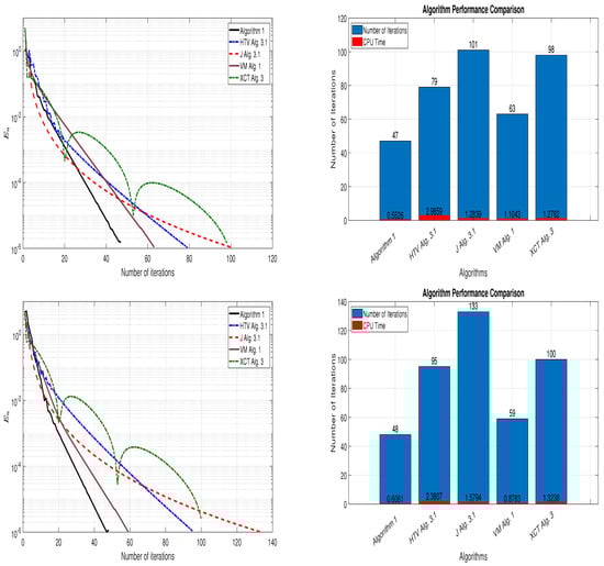
Figure 1. Norm of successive iterates ($\parallel x_n-x_{n+1}\parallel$) for the algorithms and the data in Table 1. Top: IP 1 and Bottom: IP 2.

Next, we will consider an example in the setting of the classical Banach space ${\ell }_3\left(\mathbb{R}\right)$ to support our main theorem.

Example 2.

Let $E={\ell }_3\left(\mathbb{R}\right)$ the space of cubic summable sequences given by

$${\ell }_3\left(\mathbb{R}\right)=\{s={\left\{s_i\right\}}_{i=1}^{\infty },s_i\in \mathbb{R}:\sum _{i=1}^{\infty }{\left|s_i\right|}^3<\infty \}$$

with norm ${\parallel s\parallel }_{{\ell }_3}=\sqrt[3]{{\displaystyle \sum _{i=1}^{\infty }}}{\left|s_i\right|}^3$ for all $s\in E.$ It is known that E is a Banach space, which is not a Hilbert space. Define the feasible set $\mathcal{K}$ by $\mathcal{K}:=\{s\in E:\parallel s{\parallel }_{{\ell }_3}\le 3\}$ and let the bifunction $f:\mathcal{K}\times \mathcal{K}\to \mathbb{R}$ be defined by

$$f(p,q)=(3-\parallel p\parallel )⟨p,q-p⟩,\forall p,q\in \mathcal{K}.$$

It is clear that f is pseudomonotone but not monotone and f satisfies the Lipschitz-type condition with $L=5.$ In this example, we will only compare the performance of our proposed Algorithm 1 and Jolaoso [38] (Algorithm 3.1) because other algorithms were established in the setting of Hilbert spaces. For Algorithm 1 and J Alg. 3.1, we use the same set of parameters considered in Example 1. We consider the following initial points:

IP 1. 

$r_0=x_0=x_1=(\underset{15}{\underbrace{1,1,...,1}},0,0,...)$.

IP 2. 

$r_0=x_0=x_1=(1,0.1,-1,-0.1,0,2,3,-2,-3,0,0.5,0.8,-0.3,-0.9,0.25,0,0,0,...)$ (see Table 2 and Figure 2).

Table 2. Numerical performance of all algorithms in Example 2.

Algorithms	IP 1		IP 2
	Iter.	Time (s)	Iter.	Time (s)
Algorithm 1	61	0.4822	72	0.9022
J Alg. 3.1	1801	42.287	2151	104.39

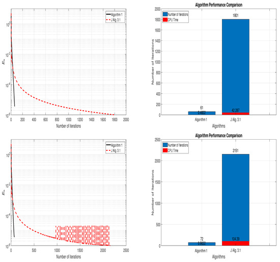Figure 2. Norm of successive iterates ($\parallel x_n-x_{n+1}\parallel$) for the algorithms and the data in Table 1. Top: IP 1 and Bottom: IP 2.

5. Conclusions

In this manuscript, we address the problem of finding approximate solutions to equilibrium problems in Banach spaces. We propose a modified proximal point algorithm that utilizes the golden ratio technique when the cost mapping is pseudomonotone. This method is self-adaptive, meaning that it does not require prior knowledge of the Lipschitz property of the operator for its control parameter. The construction of our method involves solving a single convex optimization problem in each iteration. We present and prove two convergence results: one weak convergence result and one sublinear convergence result. Lastly, we provide two numerical examples, including one conducted in a Banach space, to demonstrate the advantages of our proposed method compared to previous approaches in the literature.

References

- Blum, E.; Oettli, W. From optimization and variational inequalities to equilibrium problems. Math. Stud. 1994, 63, 123–145. [Google Scholar]
- Muu, L.; Oettli, W. Convergence of an adaptive penalty scheme for finding constrained equilibria. Nonlinear Anal. 1992, 18, 1159–1166. [Google Scholar] [CrossRef]
- Fan, K. A Minimax Inequality and Its Application; In Inequalities; Shisha, O., Ed.; Academic: New York, NY, USA, 1972; Volume 3, pp. 103–113. [Google Scholar]
- Mastroeni, G. Gap function for equilibrium problems. J. Glob. Optim. 2003, 27, 411–426. [Google Scholar] [CrossRef]
- Mastroeni, G. On Auxiliary Principle for Equilibrium Problems; Series Nonconvex Optimization and Its Applications; Springer: Berlin/Heidelberg, Germany, 2003; Volume 68, pp. 289–298. [Google Scholar]
- Moudafi, A. Proximal point algorithm extended to equilibrium problem. J. Nat. Geometry. 1999, 15, 91–100. [Google Scholar]
- Flam, S.D.; Antipin, A.S. Equilibrium programming and proximal-like algorithms. Math. Program. 1997, 78, 29–41. [Google Scholar] [CrossRef]
- Cohen, G. Auxiliary problem principle and decomposition of optimization problems. J. Optim. Theory Appl. 1980, 32, 277–305. [Google Scholar] [CrossRef]
- Tran, D.Q.; Muu, L.D.; Hien, N.V. Extragradient algorithms extended to equilibrium problems. Optimization 2008, 57, 749–776. [Google Scholar] [CrossRef]
- Korpelevich, G. An extragradient method for finding saddle points and for other problems. Ekon. Mat. Metody. 1976, 12, 747–756. [Google Scholar]
- Anh, P.N.; An, L.T.H. New subgradient extragradient methods for solving monotone bilevel equilibrium problems. Optimization 2019, 68, 2099–2124. [Google Scholar] [CrossRef]
- Anh, P.N.; An, L.T.H. The subgradient extragradient method extended to equilibrium problems. Optimization 2015, 64, 225–248. [Google Scholar] [CrossRef]
- Hieu, D.V. Halpern subgradient extragradient method extended to equilibrium problems. Rev. Real Acad. Cienc. Exactas FíSicas Nat. Ser. MatemáTicas 2017, 111, 823–840. [Google Scholar]
- Khanh, P.Q.; Thong, D.V.; Vinh, N.T. Versions of the subgradient extragradient method for pseudomonotone variational inequalities. Acta Appl. Math. 2020, 170, 319–345. [Google Scholar] [CrossRef]
- Yang, J.; Liu, H.; Liu, Z.X. Modified subgradient extragradient algorithms for solving monotone variational inequalities. Optimization 2018, 67, 2247–2258. [Google Scholar] [CrossRef]
- Yang, J.; Liu, H. The subgradient extragradient method extended to pseudomonotone equilibrium problems and fixed point problems in Hilbert space. Optim. Lett. 2019, 14, 1803–1816. [Google Scholar] [CrossRef]
- Censor, Y.; Gibali, A.; Reich, S. Extensions of Korpelevich’s extragradient method for the variational inequality problem in Euclidean space. Optimization 2012, 61, 1119–1132. [Google Scholar] [CrossRef]
- Censor, Y.; Gibali, A.; Reich, S. Strong convergence of subgradient extragradient methods for the variational inequality problem in Hilbert space. Optim. Methods Softw. 2011, 26, 827–845. [Google Scholar] [CrossRef]
- Ogbuisi, F. Popov subgradient extragradient algorithm for pseudomonotone equilibrium problem in Banach spaces. J. Nonlinear Funct. Analy. 2019, 44. [Google Scholar]
- Jolaoso, L.O.; Aphane, M. An explicit subgradient extragradient with self-adaptive stepsize for pseudomonotone equilibrium problems in Banach spaces. Numer. Algorithms 2022, 89, 583–610. [Google Scholar] [CrossRef]
- Pham Thi, H.A.; Ngo Thi, T.; Nguyen, V. The Golden ratio algorithms for solving equilibrium problems in Hilbert spaces. J. Nonlinear Var. Anal. 2021, 5, 493–518. [Google Scholar]
- Malitsky, Y. Golden ratio algorithms for variational inequalities. Math. Program. 2020, 184, 383–410. [Google Scholar] [CrossRef]
- Chang, X.K.; Yang, J.F. A golden ratio primal-dual algorithm for structured convex optimization. J. Sci. Comput. 2021, 87, 47. [Google Scholar] [CrossRef]
- Chang, X.K.; Yang, J.F.; Zhang, H.C. Golden ratio primal-dual algorithm with linesearch. SIAM J. Optim. 2022, 32, 1584–1613. [Google Scholar] [CrossRef]
- Oyewole, O.K.; Reich, S. Two subgradient extragradient methods based on the golden ratio technique for solving varia-tional inequality problems. Numer. Algorithms 2024, 97, 1215–1236. [Google Scholar] [CrossRef]
- Zhang, C.; Chu, Z. New extrapolation projection contraction algorithms based on the golden ratio for pseudo-monotone variational inequalities. AIM Math. 2023, 8, 23291–23312. [Google Scholar] [CrossRef]
- Alber, Y.I. Metric and Generalized Projection Operators in Banach Spaces: Properties and Applications; Kartsatos, A.G., Ed.; Dekker: New York, NY, USA, 1996. [Google Scholar]
- Reem, D.; Reich, S.; De Pierro, A. Re-examination of Bregman functions and new properties of their divergences. Optimization 2019, 68, 279–348. [Google Scholar] [CrossRef]
- Reich, S. A weak convergence theorem for alternating method with Bregman distance. In Theory and Applications and Nonlinear Operators of Accretive and Monotone Type; Kartsatos, A.G., Ed.; Marcel Dekker: New York, NY, USA, 1996; pp. 313–318. [Google Scholar]
- Goebel, K.; Reich, S. Uniform Convexity, Hyperbolic Geometry, and Nonexpansive Mappings; Marcel Dekker: New York, NY, USA; Basel, Switzerland, 1984. [Google Scholar]
- Cioranescu, I. Geometry of Banach Spaces, Duality Mappings, and Nonlinear Problems; Kluwer: Dordrecht, The Netherlands, 1990. [Google Scholar]
- Kamimura, S.; Takahashi, W. Strong convergence of a proximal-type algorithm in Banach space. SIAM J. Optim. 2002, 13, 938–945. [Google Scholar] [CrossRef]
- Nakajo, K. Strong convergence for gradient projection method and relatively nonexpansive mappings in Banach spaces. Appl. Math. Comput. 2015, 271, 251–258. [Google Scholar] [CrossRef]
- Avetisyan, K.; Djordjević, K.; Pavlović, M. Littlewood-palew inequalities in uniformly convex and uniformly smooth Banach spaces. J. Math. Anal. Appl. 2007, 336, 31–43. [Google Scholar] [CrossRef]
- Tiel, J.V. Convex Analysis: An Introductory Text; Wiley: New York, NY, USA, 1984. [Google Scholar]
- Parikh, N.; Boyd, S. Proximal Algorithms. Found. Trends Optim. 2013, 1, 123–231. [Google Scholar]
- Acedo, G.L.; Xu, H.K. Iterative methods for strict pseudo-contractions in Hilbert spaces. Nonlinear Anal. 2007, 67, 2258–2271. [Google Scholar] [CrossRef]
- Jolaoso, L.O. The subgradient extragradient method for solving pseudomonotone equilibrium and fixed point problems in Banach spaces. Optimization 2022, 71, 4051–4081. [Google Scholar] [CrossRef]
- Vinh, N.T.; Muu, L.D. Inertial extragradient algorithms for solving equilibrium problems. Acta Math. Vietnam. 2019, 44, 639–663. [Google Scholar] [CrossRef]
- Xie, Z.; Cai, G.; Tan, B. Inertial subgradient extragradient method for solving pseudomonotone equilibrium problems and fixed point problems in Hilbert spaces. Optimization 2022, 73, 1329–1354. [Google Scholar] [CrossRef]
Disclaimer/Publisher’s Note: The statements, opinions and data contained in all publications are solely those of the individual author(s) and contributor(s) and not of MDPI and/or the editor(s). MDPI and/or the editor(s) disclaim responsibility for any injury to people or property resulting from any ideas, methods, instructions or products referred to in the content. |
© 2024 by the authors. Licensee MDPI, Basel, Switzerland. This article is an open access article distributed under the terms and conditions of the Creative Commons Attribution (CC BY) license (https://creativecommons.org/licenses/by/4.0/).