On the Dynamics of Some Higher-Order Nonlinear Difference Equations

Abstract

This research investigates the dynamics of higher-order nonlinear difference equations, specifically concentrating on seventh-order instances. Analytical solutions are obtained for particular equations, a formidable task owing to the absence of explicit mathematical techniques for their resolution. The qualitative characteristics of solutions, such as their stability, boundedness, and periodicity, are analysed by theoretical methods and numerical simulations. The results indicate that equilibrium points frequently lack local asymptotic stability, leading to intricate phenomena such as unbounded solutions and periodic attractors. These findings augment our understanding of nonlinear difference equations, offering significant implications for their use across various scientific fields.

1. Introduction

Recently, difference equations have been considered one of the most used equations for modeling phenomena. Since difference equations have many features to provide more accurate predictions, scientists tend to use them in their models in different fields of research, such as population dynamics and genetics in biology, hypergeometric Poisson distributions in probability problems, etc. However, there are two ways to study difference equations. The first is by analyzing the qualitative behavior of solutions, for example, investigating the solutions’ stability, boundedness, and periodicity. So, several articles have been published for studying rational difference equations in this case, for instance, the following recent studies:

Kerker et al. [1] discussed boundedness and global solutions. Also, an oscillation result for positive solutions was obtained for the higher-order non-autonomous difference equation

$$y_{n+1}={\displaystyle \frac{{\alpha }_n+y_{n-l}}{{\alpha }_n+y_{n-k}}},n=0,1,\dots .$$

In [2], the local and global stability and periodicity were examined in the fourth-order nonlinear difference equation

$$x_{n+1}=a{x}_{n-1}-{\displaystyle \frac{b{x}_{n-1}}{c{x}_{n-1}-d{x}_{n-3}}},n=0,1,\dots .$$

Garic-Demirovic et al. [3] investigated the bifurcation of a fixed point in a special case involving complex conjugate numbers and the local stability and global attractivity of period-two solutions of a homogeneous fractional difference equation and the unique equilibrium point of

$$x_{n+1}={\displaystyle \frac{A{x}_n^2+B{x}_n{x}_{n-1}+C{x}_{n-1}^2}{a{x}_n^2+b{x}_n{x}_{n-1}+c{x}_{n-1}^2}},n=0,1,\dots .$$

The second method is to obtain the form of solutions, which is more challenging for researchers since there is no explicit mathematical method for solving nonlinear difference equations. Therefore, there exists a great interest in studying difference equations by structuring the solutions’ forms. Some recent papers are presented as follows:

Tollu et al. [4] derived a closed-form solution and analyzed the asymptotic behavior of the solutions to the nonlinear difference equation

$$x_n=a{x}_{n-k}+{\displaystyle \frac{\delta x_{n-k}{x}_{n-(k+1)}}{\beta x_{n-(k+1)}+\gamma x_{n-1}}},n=0,1,\dots ..$$

El-Metwally et al. [5] looked into some of the qualitative behavior of the solutions such as the the global stability, boundedness, and periodicity characteristic for rational recursive sequences:

$$x_{n+1}={\displaystyle \frac{x_n{x}_{n-3}}{x_{n-2}(\pm 1\pm x_n{x}_{n-3})}},n=0,1,\dots .$$

Jia [6] investigated the equilibrium point’s asymptotic stability, as well as establishing criteria for the solution’s positivity for the following high-order fuzzy difference equation:

$$X_{n+1}={\displaystyle \frac{A_1{X}_{n-1}{X}_{n-2}}{B_2{\sum }_{i=3}^k{C}_i{X}_{n-i}}},n=0,1,\dots .$$

Kara et al. [7] explored the closed-form solution and discussed the dynamics of some cases of the following system:

$$x_n=a{y}_{n-k}+{\displaystyle \frac{d{y}_{n-k}{x}_{n-(k+l)}}{b{x}_{n-(k+l)}+c{y}_{n-l}}},y_n=\alpha x_{n-k}+{\displaystyle \frac{\delta x_{n-k}{y}_{n-(k+l)}}{\beta y_{n-(k+l)}+\gamma x_{n-l}}}$$

For additional research in this area, we direct the reader to [8,9,10,11,12,13,14,15,16,17,18,19,20,21,22,23,24,25,26,27,28,29,30,31] and the sources listed therein.

In this paper, we modified [5] to a seventh-order nonlinear difference equation and derived explicit solutions to some cases of difference equations, which are listed below and whose analytical solutions are usually a major challenge for researchers. In addition, a comprehensive analysis of the qualitative properties of the solutions, such as their stability, boundedness, and periodicity, is provided through both the theoretical results and numerical simulations.

$$Y_{n+1}={\displaystyle \frac{Y_{n-5}{Y}_{n-6}}{Y_n(\pm 1\pm Y_{n-1}{Y}_{n-2}{Y}_{n-3}{Y}_{n-4}{Y}_{n-5}{Y}_{n-6})}},n=0,1,\dots .$$

(1)

where the initial values $Y_i$ for $(i=0,-1,-2,-3,-4,-5,-6)$ are arbitrary real numbers.

This paper is arranged as follows: In Section 2, we recall some fundamental definitions and theorems from difference equations. Section 3 is designed to discuss the dynamics of the first case of (1). In Section 4, we illustrate the explicit solution and investigate the periodic behavior of the second case of (1). Section 5 and Section 6 contain the results for the last two cases of (1). We provide some numerical simulations in Section 7. The discussion about the findings is given in Section 8.

2. Definitions and Fundamental Theorems

In this phase, we review certain concepts and conclusions from the theory of difference equations that will be utilized in our investigation. Suppose J is a continuously differentiable function such that $J:{[a,b]}^{k+1}\to [a,b]$, where $[a,b]$ is a real number interval and k is a positive integer. Then, the difference equation

$$Y_{n+1}=J(Y_n,Y_{n-1},\dots ,Y_{n-k}),n=0,1,2,\dots$$

(2)

has a unique solution ${\left\{Y_n\right\}}_{n=-k}^{\infty }$ for all sets of inital values $Y_{-k},Y_{-k+1},\dots ,Y_0\in [a,b]$ [32].

Definition 1.

A point $Y^{\ast }\in [a,b]$ is called an equilibrium point of Equation (2) if

$$Y^{\ast }=J(Y^{\ast },Y^{\ast },\dots ,Y^{\ast }).$$

That is, $Y_n=Y^{\ast }$, for all $n\ge 0$, is a solution of Equation (8), or, equivalently, $Y^{\ast }$ is a fixed point of J.

Definition 2.

The equilibrium point $Y^{\ast }$ of Equation (2) is said to be

• Locally stable if, for every $\alpha >0$, there exists $\beta >0$ such that for every $Y_{-k},Y_{-k+1},\dots ,Y_{-1},Y_0\in [a,b]$, with

  $$|Y_{-k}-Y^{\ast }|+|Y_{-k+1}-Y^{\ast }|+\dots +|Y_0-Y^{\ast }|<\beta ,$$

  we have

  $$|Y_n-Y^{\ast }|<\alpha \forall n\ge -k.$$
• Locally asymptotically stable if $Y^{\ast }$ is a locally stable solution of Equation (2) and there exists $\mu >0$ such that for every $Y_{-k},Y_{-k+1},\dots ,Y_{-1},Y_0\in [a,b]$, with

  $$|Y_{-k}-Y^{\ast }|+|Y_{-k+1}-Y^{\ast }|+\dots +|Y_0-Y^{\ast }|<\mu ,$$

  we have

  $$\underset{n\to \infty }{lim}{Y}_n=Y^{\ast }.$$
• A global attractor if, for every $Y_{-k},Y_{-k+1},\dots ,Y_{-1},Y_0\in [a,b]$, we have

  $$\underset{n\to \infty }{lim}{Y}_n=Y^{\ast }.$$
• Globally asymptotically stable if $Y^{\ast }$ is locally stable and also a global attractor of Equation (2).
• Unstable if $Y^{\ast }$ is not a locally stable solution of Equation (2).

Definition 3.

A sequence ${\left\{Y_n\right\}}_{n=-k}^{\infty }$ is a periodic solution with a period q if $Y_{n+q}=Y_n$ for all $n\ge -k$.

Theorem 1

(Kocic and Ladas [33]). Assume that ${\lambda }_i\in R$, where $i=1,2,3,\dots ,k$ and $k\in \{0,1,2,3,\dots \}$. Then,

$${\displaystyle \sum _{i=1}^k}\left|{\lambda }_i\right|<1$$

is a sufficient condition for the asymptotic stability of the following difference equation

$$Y_{n+k}+{\lambda }_1{Y}_{n+k-1}+\dots +{\lambda }_k{Y}_n=0,n=0,1,2,\dots .$$

3. The First Case

This section discusses the equilibrium point and the state of stability. Also, a specific form of solution will be clarified for the following difference equation:

$$Y_{n+1}={\displaystyle \frac{Y_{n-5}{Y}_{n-6}}{Y_n(1+Y_{n-1}{Y}_{n-2}{Y}_{n-3}{Y}_{n-4}{Y}_{n-5}{Y}_{n-6})}},n=0,1,\dots .$$

(3)

where the initial values are arbitrary real numbers.

Theorem 2.

The equilibrium point $Y^{\ast }$ of difference Equation (3) has a unique zero value.

Proof. 

Equation (3) can be written as

$$Y^{\ast }={\displaystyle \frac{Y^{\ast 2}}{Y^{\ast }(1+Y^{\ast 6})}},$$

or

$$Y^{\ast 2}(1+Y^{\ast 6})-Y^{\ast 2}=0,$$

which implies

$$Y^{\ast 2}(1+Y^{\ast 6}-1)=0.$$

Therefore, the equilibrium point of the difference Equation (3) is unique. □

Theorem 3.

The equilibrium point $Y^{\ast }$ of difference Equation (3) is not locally asymptotically stable.

Proof. 

Suppose that $J:{(0,\infty )}^7\to (0,\infty )$ is a function defined as follows:

$$J(\alpha ,\beta ,\gamma ,\kappa ,\rho ,\zeta ,\mu )={\displaystyle \frac{\zeta \mu }{\alpha (1+\beta \gamma \kappa \rho \zeta \mu )}}.$$

(4)

After differentiating $J(\alpha ,\beta ,\gamma ,\kappa ,\rho ,\zeta ,\mu )$ with respect to $\alpha$, $\beta$, $\gamma$, $\kappa$, $\rho$, $\zeta$, and $\mu$, we obtain

$$\begin{array}{cccc}\hfill J_{\alpha }(\alpha ,\beta ,\gamma ,\kappa ,\rho ,\zeta ,\mu )& ={\displaystyle \frac{-\zeta \mu }{{\alpha }^2(1+\beta \gamma \kappa \rho \zeta \mu )}}={\lambda }_1,\hfill & \hfill J_{\beta }(\alpha ,\beta ,\gamma ,\kappa ,\rho ,\zeta ,\mu )& ={\displaystyle \frac{-{\zeta }^2{\mu }^2\gamma \kappa \rho }{\alpha {(1+\beta \gamma \kappa \rho \zeta \mu )}^2}}={\lambda }_2,\hfill \\ \hfill J_{\gamma }(\alpha ,\beta ,\gamma ,\kappa ,\rho ,\zeta ,\mu )& ={\displaystyle \frac{-{\zeta }^2{\mu }^2\beta \kappa \rho }{\alpha {(1+\beta \gamma \kappa \rho \zeta \mu )}^2}}={\lambda }_3,\hfill & \hfill J_{\kappa }(\alpha ,\beta ,\gamma ,\kappa ,\rho ,\zeta ,\mu )& ={\displaystyle \frac{-{\zeta }^2{\mu }^2\beta \gamma \rho }{\alpha {(1+\beta \gamma \kappa \rho \zeta \mu )}^2}}={\lambda }_4,\hfill \\ \hfill J_{\rho }(\alpha ,\beta ,\gamma ,\kappa ,\rho ,\zeta ,\mu )& ={\displaystyle \frac{-{\zeta }^2{\mu }^2\beta \gamma \kappa }{\alpha {(1+\beta \gamma \kappa \rho \zeta \mu )}^2}}={\lambda }_5,\hfill & \hfill f_{\zeta }(\alpha ,\beta ,\gamma ,\kappa ,\rho ,\zeta ,\mu )& ={\displaystyle \frac{\mu }{\alpha {(1+\beta \gamma \kappa \rho \zeta \mu )}^2}}={\lambda }_6,\hfill \\ \hfill J_{\mu }(\alpha ,\beta ,\gamma ,\kappa ,\rho ,\zeta ,\mu )& ={\displaystyle \frac{\zeta }{\alpha {(1+\beta \gamma \kappa \rho \zeta \mu )}^2}}={\lambda }_7.\hfill & & \end{array}$$

Now, by substituting $Y^{\ast }$ into ${\lambda }_i$ for $i=1,\dots ,7$, we obtain

$$\begin{array}{cccc}\hfill J_{\alpha }(Y^{\ast },Y^{\ast },Y^{\ast },Y^{\ast },Y^{\ast },Y^{\ast },Y^{\ast })& =-1,\hfill & \hfill J_{\beta }(Y^{\ast },Y^{\ast },Y^{\ast },Y^{\ast },Y^{\ast },Y^{\ast },Y^{\ast })& =0,\hfill \\ \hfill J_{\gamma }(Y^{\ast },Y^{\ast },Y^{\ast },Y^{\ast },Y^{\ast },Y^{\ast },Y^{\ast })& =0,\hfill & \hfill J_{\kappa }(Y^{\ast },Y^{\ast },Y^{\ast },Y^{\ast },Y^{\ast },Y^{\ast },Y^{\ast })& =0,\hfill \\ \hfill J_{\rho }(Y^{\ast },Y^{\ast },Y^{\ast },Y^{\ast },Y^{\ast },Y^{\ast },Y^{\ast })& =0,\hfill & \hfill J_{\zeta }(Y^{\ast },Y^{\ast },Y^{\ast },Y^{\ast },Y^{\ast },Y^{\ast },Y^{\ast })& =1,\hfill \\ \hfill J_{\mu }(Y^{\ast },Y^{\ast },Y^{\ast },Y^{\ast },Y^{\ast },Y^{\ast },Y^{\ast })& =1.\hfill & & \end{array}$$

Therefore, the linearized equation of (3) regarding the equilibrium point $Y^{\ast }$ is as follows:

$$Y_{n+1}+{\lambda }_1{Y}_n+{\lambda }_2{Y}_{n-1}+{\lambda }_3{Y}_{n-2}+{\lambda }_4{Y}_{n-3}+{\lambda }_5{Y}_{n-4}+{\lambda }_6{Y}_{n-5}+{\lambda }_7{Y}_{n-6}=0.$$

(5)

Therefore, by using Theorem 1, we find that the equilibrium point of Equation (3) is not locally asymptotically stable. □

Form of Solution

The solution of Equation (3) is obtained in a specific form.

Theorem 4.

Assume ${\left\{Y_n\right\}}_{n=-6}^{\infty }$ is a solution of (3) and suppose that $Y_0=a$, $Y_{-1}=b$, $Y_{-2}=c$, $Y_{-3}=d$, $Y_{-4}=e$, $Y_{-5}=f$, and $Y_{-6}=g$.

Then, Equation (3)’s solution can be derived in the following manner for $n⩾0$:

$$Y_{6n-6}={\displaystyle \frac{a^n}{g^{n-1}}}{\displaystyle \prod _{i=0}^{n-2}}\left({\displaystyle \frac{1+(3i+3)bcdefg}{1+(3i+3)abcdef}}\right).$$

$$Y_{6n-5}={\displaystyle \frac{f{g}^n}{a^n}}{\displaystyle \prod _{i=0}^{n-1}}\left({\displaystyle \frac{1+3iabcdef}{1+(3i+1)bcdefg}}\right),$$

$$Y_{6n-4}={\displaystyle \frac{e{a}^n}{g^n}}{\displaystyle \prod _{i=0}^{n-1}}\left({\displaystyle \frac{1+(3i+1)bcdefg}{1+(3i+1)abcdef}}\right),$$

$$Y_{6n-3}={\displaystyle \frac{d{g}^n}{a^n}}{\displaystyle \prod _{i=0}^{n-1}}\left({\displaystyle \frac{1+(3i+1)abcdef}{1+(3i+2)bcdefg}}\right),$$

$$Y_{6n-2}={\displaystyle \frac{c{a}^n}{g^n}}{\displaystyle \prod _{i=0}^{n-1}}\left({\displaystyle \frac{1+(3i+2)bcdefg}{1+(3i+2)abcdef}}\right),$$

$$Y_{6n-1}={\displaystyle \frac{b{g}^n}{a^n}}{\displaystyle \prod _{i=0}^{n-1}}\left({\displaystyle \frac{1+(3i+2)abcdef}{1+(3i+3)bcdefg}}\right),$$

$$Y_{6n}={\displaystyle \frac{a^{n+1}}{g^n}}{\displaystyle \prod _{i=0}^{n-1}}\left({\displaystyle \frac{1+(3i+3)bcdefg}{1+(3i+3)abcdef}}\right).$$

Proof. 

It is clear that for $n=0$, the result is true. Now for $n>0$, assume the result holds for $n-1$ and it is given as follows:

$$Y_{6n-12}={\displaystyle \frac{a^{n-1}}{g^{n-2}}}{\displaystyle \prod _{i=0}^{n-3}}\left({\displaystyle \frac{1+(3i+3)bcdefg}{1+(3i+3)abcdef}}\right),$$

$$Y_{6n-11}={\displaystyle \frac{f{g}^{n-1}}{a^{n-1}}}{\displaystyle \prod _{i=0}^{n-2}}\left({\displaystyle \frac{1+3iabcdef}{1+(3i+1)bcdefg}}\right),$$

$$Y_{6n-10}={\displaystyle \frac{e{a}^{n-1}}{g^{n-1}}}{\displaystyle \prod _{i=0}^{n-2}}\left({\displaystyle \frac{1+(3i+1)bcdefg}{1+(3i+1)abcdef}}\right),$$

$$Y_{6n-9}={\displaystyle \frac{d{g}^{n-1}}{a^{n-1}}}{\displaystyle \prod _{i=0}^{n-2}}\left({\displaystyle \frac{1+(3i+1)abcdef}{1+(3i+2)bcdefg}}\right),$$

$$Y_{6n-8}={\displaystyle \frac{c{a}^{n-1}}{g^{n-1}}}{\displaystyle \prod _{i=0}^{n-2}}\left({\displaystyle \frac{1+(3i+2)bcdefg}{1+(3i+2)abcdef}}\right),$$

$$Y_{6n-7}={\displaystyle \frac{b{g}^{n-1}}{a^{n-1}}}{\displaystyle \prod _{i=0}^{n-2}}\left({\displaystyle \frac{1+(3i+2)abcdef}{1+(3i+3)bcdefg}}\right),$$

$$Y_{6n-6}={\displaystyle \frac{a^n}{g^{n-1}}}{\displaystyle \prod _{i=0}^{n-2}}\left({\displaystyle \frac{1+(3i+3)bcdefg}{1+(3i+3)abcdef}}\right).$$

Now, the first relation will be proven.

After substituting $6n-5$ into Equation (3), we obtain

$$Y_{6n-5}={\displaystyle \frac{Y_{6n-11}{Y}_{6n-12}}{Y_{6n-6}(1+Y_{6n-7}{Y}_{6n-8}{Y}_{6n-9}{Y}_{6n-10}{Y}_{6n-11}{Y}_{6n-12})}}.$$

(6)

Substituting in the values of $Y_{6n-6},Y_{6n-7},Y_{6n-8},Y_{6n-9},Y_{6n-10},Y_{6n-11}$, and $Y_{6n-12}$ gives

$$Y_{6n-5}={\displaystyle \frac{f{g}^n{\prod }_{i=0}^{n-2}\left(\frac{1}{1+(3i+1)bcdefg}\right){\prod }_{i=0}^{n-3}\left(\frac{1+(3i+3)bcdefg}{1}\right)}{a^n{\prod }_{i=0}^{n-2}\left(\frac{1+(3i+3)bcdefg}{1+(3i+3)abcdef}\right)\left(\begin{array}{c}1+\frac{bcdefg}{1+(3n-3)bcdefg}\end{array}\right)}},$$

$$Y_{6n-5}={\displaystyle \frac{f{g}^n{\prod }_{i=0}^{n-2}\left(\frac{1+(3i+3)abcdef}{1+(3i+1)bcdefg}\right)}{a^n(1+(3n-3)bcdefg)\left(\begin{array}{c}1+\frac{bcdefg}{1+(3n-3)bcdefg}\end{array}\right)}},$$

so

$$Y_{6n-5}={\displaystyle \frac{f{g}^n{\prod }_{i=0}^{n-2}\left(\frac{1+(3i+3)abcdef}{1+(3i+1)bcdefg}\right)}{a^n(1+(3n-3)bcdefg+bcdefg)}},$$

$$Y_{6n-5}={\displaystyle \frac{f{g}^n}{a^n}}{\displaystyle \prod _{i=0}^{n-2}}\left({\displaystyle \frac{1+(3i+3)abcdef}{(1+(3i+1\left)bcdefg\right)(1+(3n-2\left)bcdefg\right)}}\right).$$

Consequently,

$$Y_{6n-5}={\displaystyle \frac{f{g}^n}{a^n}}{\displaystyle \prod _{i=0}^{n-1}}\left({\displaystyle \frac{1+3iabcdef}{1+(3i+1)bcdefg}}\right).$$

Similarly, we can prove the second form.

From Equation (3), we see that

$$Y_{6n-4}={\displaystyle \frac{Y_{6n-10}{Y}_{6n-11}}{Y_{6n-5}(1+Y_{6n-6}{Y}_{6n-7}{Y}_{6n-8}{Y}_{6n-9}{Y}_{6n-10}{Y}_{6n-11})}},$$

(7)

which implies that

$$Y_{6n-4}={\displaystyle \frac{e{a}^n{\prod }_{i=0}^{n-2}\left(\frac{1}{1+(3i+1)abcdef}\right){\prod }_{i=0}^{n-2}\left(\frac{1+3iabcdef}{1}\right)}{g^n{\prod }_{i=0}^{n-1}\left(\frac{1+3iabcdef}{1+(3i+1)bcdefg}\right)\left(\begin{array}{c}1+\frac{abcdef}{1+(3n-3)acdef}\end{array}\right)}},$$

$$Y_{6n-4}={\displaystyle \frac{e{a}^n{\prod }_{i=0}^{n-2}\left(\frac{1}{1+(3i+1)abcdef}\right){\prod }_{i=0}^{n-1}(1+(3i+1)bcdefg)}{g^n(1+(3n-3)abcdef+abcdef)}},$$

i.e,

$$Y_{6n-4}={\displaystyle \frac{e{a}^n{\prod }_{i=0}^{n-1}(1+(3i+1)bcdefg)}{g^n{\prod }_{i=0}^{n-2}(1+(3i+1)abcdef)(1+(3n-2)abcdef)}}.$$

Thus,

$$Y_{6n-4}={\displaystyle \frac{e{a}^n}{g^n}}{\displaystyle \prod _{i=0}^{n-1}}\left({\displaystyle \frac{1+(3i+1)bcdefg}{1+(3i+1)abcdef}}\right).$$

The remaining forms can be verified using the same approach. The proof is complete. □

4. The Second Case

The calculation of equilibrium points and their state of stability is shown in this part for the following difference equation:

$$Y_{n+1}={\displaystyle \frac{Y_{n-5}{Y}_{n-6}}{Y_n(-1+Y_{n-1}{Y}_{n-2}{Y}_{n-3}{Y}_{n-4}{Y}_{n-5}{Y}_{n-6})}},n=0,1,\dots ,$$

(8)

where the initial values are arbitrary non-zero real numbers with $Y_0{Y}_{-1}{Y}_{-2}{Y}_{-3}{Y}_{-4}{Y}_{-5}\ne 1$ and $Y_{-1}{Y}_{-2}{Y}_{-3}{Y}_{-4}{Y}_{-5}{Y}_{-6}\ne 1$.

Theorem 5.

Difference Equation (8) has three equilibrium points $Y^{\ast }$, which are 0 and $\pm \sqrt[6]{2}$.

Proof. 

We can write Equation (8) as

$$Y^{\ast }={\displaystyle \frac{Y^{\ast 2}}{Y^{\ast }(-1+Y^{\ast 6})}},$$

i.e.,

$$Y^{\ast 2}(-1+Y^{\ast 6})-Y^{\ast 2}=0,$$

$$Y^{\ast 2}(-1+Y^{\ast 6}-1)=0.$$

Thus,

$$Y^{\ast 2}(Y^{\ast 6}-2)=0.$$

Hence, difference Equation (8) has three equilibrium points—$Y_1^{\ast }=0,Y_2^{\ast }=\sqrt[6]{2}$, and $Y_3^{\ast }=-\sqrt[6]{2}$. □

Theorem 6.

The equilibrium points $Y_{1,2,3}^{\ast }$ of difference Equation (8) are not locally asymptotically stable.

Proof. 

Suppose that $J:{(0,\infty )}^7\to (0,\infty )$ is a function defined as follows:

$$J(\alpha ,\beta ,\gamma ,\kappa ,\rho ,\zeta ,\mu )={\displaystyle \frac{\zeta \mu }{\alpha (-1+\beta \gamma \kappa \rho \zeta \mu )}}.$$

(9)

After differentiating $J(\alpha ,\beta ,\gamma ,\kappa ,\rho ,\zeta ,\mu )$ with respect to $\alpha$, $\beta$, $\gamma$, $\kappa$, $\rho$, $\zeta$, and $\mu$, we obtain

$$\begin{array}{cccc}\hfill J_{\alpha }(\alpha ,\beta ,\gamma ,\kappa ,\rho ,\zeta ,\mu )& ={\displaystyle \frac{-\zeta \mu }{{\alpha }^2(-1+\beta \gamma \kappa \rho \zeta \mu )}}={\lambda }_1,\hfill & \hfill J_{\beta }(\alpha ,\beta ,\gamma ,\kappa ,\rho ,\zeta ,\mu )& ={\displaystyle \frac{-{\zeta }^2{\mu }^2\gamma \kappa \rho }{\alpha {(-1+\beta \gamma \kappa \rho \zeta \mu )}^2}}={\lambda }_2,\hfill \\ \hfill J_{\gamma }(\alpha ,\beta ,\gamma ,\kappa ,\rho ,\zeta ,\mu )& ={\displaystyle \frac{-{\zeta }^2{\mu }^2\beta \kappa \rho }{\alpha {(-1+\beta \gamma \kappa \rho \zeta \mu )}^2}}={\lambda }_3,\hfill & \hfill J_{\kappa }(\alpha ,\beta ,\gamma ,\kappa ,\rho ,\zeta ,\mu )& ={\displaystyle \frac{-{\zeta }^2{\mu }^2\beta \gamma \rho }{\alpha {(-1+\beta \gamma \kappa \rho \zeta \mu )}^2}}={\lambda }_4,\hfill \\ \hfill J_{\rho }(\alpha ,\beta ,\gamma ,\kappa ,\rho ,\zeta ,\mu )& ={\displaystyle \frac{-{\zeta }^2{\mu }^2\beta \gamma \kappa }{\alpha {(-1+\beta \gamma \kappa \rho \zeta \mu )}^2}}={\lambda }_5,\hfill & \hfill f_{\zeta }(\alpha ,\beta ,\gamma ,\kappa ,\rho ,\zeta ,\mu )(& ={\displaystyle \frac{-\mu }{\alpha {(-1+\beta \gamma \kappa \rho \zeta \mu )}^2}}={\lambda }_6,\hfill \\ \hfill J_{\mu }(\alpha ,\beta ,\gamma ,\kappa ,\rho ,\zeta ,\mu )& ={\displaystyle \frac{-\zeta }{\alpha {(-1+\beta \gamma \kappa \rho \zeta \mu )}^2}}={\lambda }_7.\hfill & & \end{array}$$

Now, substituting $Y_{1,2,3}^{\ast }$ into ${\lambda }_i$ for $i=1,\dots ,7$, we obtain

$$\begin{array}{cccc}\hfill J_{\alpha }(\alpha ,\beta ,\gamma ,\kappa ,\rho ,\zeta ,\mu )\left(Y_{1,2,3}^{\ast }\right)& =\pm 1,\hfill & \hfill J_{\beta }(\alpha ,\beta ,\gamma ,\kappa ,\rho ,\zeta ,\mu )\left(Y_{1,2,3}^{\ast }\right)& =0or-2,\hfill \\ \hfill J_{\rho }(\alpha ,\beta ,\gamma ,\kappa ,\rho ,\zeta ,\mu )\left(Y_{1,2,3}^{\ast }\right)& =0,or-2,\hfill & \hfill J_{\kappa }(\alpha ,\beta ,\gamma ,\kappa ,\rho ,\zeta ,\mu )\left(Y_{1,2,3}^{\ast }\right)& =0,or-2,\hfill \\ \hfill J_{\gamma }(\alpha ,\beta ,\gamma ,\kappa ,\rho ,\zeta ,\mu )\left(Y_{1,2,3}^{\ast }\right)& =0or-2,\hfill & \hfill J_{\zeta }(\alpha ,\beta ,\gamma ,\kappa ,\rho ,\zeta ,\mu )\left(Y_{1,2,3}^{\ast }\right)& =\pm 1,\hfill \\ \hfill J_{\mu }(\alpha ,\beta ,\gamma ,\kappa ,\rho ,\zeta ,\mu )\left(Y_{1,2,3}^{\ast }\right)& =\pm 1.\hfill & & \end{array}$$

Hence, the linearized equation of (8) about the equilibrium points $Y_{1,2,3}^{\ast }$ is

$$Y_{n+1}+{\lambda }_1{Y}_n+{\lambda }_2{Y}_{n-1}+{\lambda }_3{Y}_{n-2}+{\lambda }_4{Y}_{n-3}+{\lambda }_5{Y}_{n-4}+{\lambda }_6{Y}_{n-5}+{\lambda }_7{Y}_{n-6}=0.$$

(10)

Therefore, we find that the equilibrium points of Equation (8) are not locally stable using Theorem 1. The proof is complete. □

Form of Solution

In this part, the form of the solution to the difference Equation (8) is demonstrated.

Theorem 7.

Let ${\left\{Y_n\right\}}_{n=-6}^{\infty }$ be a solution of (8) and suppose that $Y_0=a$, $Y_{-1}=b$, $Y_{-2}=c$, $Y_{-3}=d$, $Y_{-4}=e$, $Y_{-5}=f$, and $Y_{-6}=g$. Then, for $n⩾0$, the solution of Equation (8) can be formed as follows:

$$Y_{12n-5}={\displaystyle \frac{f{g}^{2n}{(-1+abcdef)}^n}{a^{2n}{(-1+bcdefg)}^n}},Y_{12n+1}={\displaystyle \frac{f{g}^{2n+1}{(-1+abcdef)}^n}{a^{2n+1}{(-1+bcdefg)}^{n+1}}},$$

$$Y_{12n-4}={\displaystyle \frac{e{a}^{2n}{(-1+bcdefg)}^n}{g^{2n}{(-1+abcdef)}^n}},Y_{12n+2}={\displaystyle \frac{e{a}^{2n+1}{(-1+bcdefg)}^{n+1}}{g^{2n+1}{(-1+abcdef)}^{n+1}}},$$

$$Y_{12n-3}={\displaystyle \frac{d{g}^{2n}{(-1+abcdef)}^n}{a^{2n}{(-1+bcdefg)}^n}},Y_{12n+3}={\displaystyle \frac{d{g}^{2n+1}{(-1+abcdef)}^{n+1}}{a^{2n+1}{(-1+bcdefg)}^n}},$$

$$Y_{12n-2}={\displaystyle \frac{c{a}^{2n}{(-1+bcdefg)}^n}{g^{2n}{(-1+abcdef)}^n}},Y_{12n+4}={\displaystyle \frac{c{a}^{2n+1}{(-1+bcdefg)}^n}{g^{2n+1}{(-1+abcdef)}^n}},$$

$$Y_{12n-1}={\displaystyle \frac{b{g}^{2n}{(-1+abcdef)}^n}{a^{2n}{(-1+bcdefg)}^n}},Y_{12n+5}={\displaystyle \frac{b{g}^{2n+1}{(-1+abcdef)}^n}{a^{2n+1}{(-1+bcdefg)}^{n+1}}},$$

$$Y_{12n}={\displaystyle \frac{a^{2n+1}{(-1+bcdefg)}^n}{g^{2n}{(-1+abcdef)}^n}},Y_{12n+6}={\displaystyle \frac{a^{2n+2}{(-1+bcdefg)}^{n+1}}{g^{2n+1}{(-1+abcdef)}^{n+1}}}.$$

Proof. 

It is clear that at $n=0$, the result is true. Now, for $n>0$, assume the result is true at $n-1$ and it is given as follows:

$$Y_{12n-17}={\displaystyle \frac{f{g}^{2n-2}{(-1+abcdef)}^{n-1}}{a^{2n-2}{(-1+bcdefg)}^{n-1}}},Y_{12n-11}={\displaystyle \frac{f{g}^{2n-1}{(-1+abcdef)}^{n-1}}{a^{2n-1}{(-1+bcdefg)}^n}},$$

$$Y_{12n-16}={\displaystyle \frac{e{a}^{2n-2}{(-1+bcdefg)}^{n-1}}{g^{2n-2}{(-1+abcdef)}^{n-1}}},Y_{12n-10}={\displaystyle \frac{e{a}^{2n-1}{(-1+bcdefg)}^n}{g^{2n-1}{(-1+abcdef)}^n}},$$

$$Y_{12n-15}={\displaystyle \frac{d{g}^{2n-2}{(-1+abcdef)}^{n-1}}{a^{2n-2}{(-1+bcdefg)}^{n-1}}},Y_{12n-9}={\displaystyle \frac{d{g}^{2n-1}{(-1+abcdef)}^n}{a^{2n-1}{(-1+bcdefg)}^{n-1}}},$$

$$Y_{12n-14}={\displaystyle \frac{c{a}^{2n-2}{(-1+bcdefg)}^{n-1}}{g^{2n-2}{(-1+abcdef)}^{n-1}}},Y_{12n-8}={\displaystyle \frac{c{a}^{2n-1}{(-1+bcdefg)}^{n-1}}{g^{2n-1}{(-1+abcdef)}^{n-1}}},$$

$$Y_{12n-13}={\displaystyle \frac{b{g}^{2n-2}{(-1+abcdef)}^{n-1}}{a^{2n-2}{(-1+bcdefg)}^{n-1}}},Y_{12n-7}={\displaystyle \frac{b{g}^{2n-1}{(-1+abcdef)}^{n-1}}{a^{2n-1}{(-1+bcdefg)}^n}},$$

$$Y_{12n-12}={\displaystyle \frac{a^{2n-1}{(-1+bcdefg)}^{n-1}}{g^{2n-2}{(-1+abcdef)}^{n-1}}},Y_{12n-6}={\displaystyle \frac{a^{2n}{(-1+bcdefg)}^n}{g^{2n-1}{(-1+abcdef)}^n}}.$$

Now, the first form will be established.

Substituting $6n-5$ into Equation (8), we obtain

$$Y_{12n-5}={\displaystyle \frac{Y_{12n-11}{Y}_{12n-12}}{Y_{12n-6}(-1+Y_{12n-7}{Y}_{12n-8}{Y}_{12n-9}{Y}_{12n-10}{Y}_{12n-11}{Y}_{12n-12})}},$$

(11)

Substituting in the values of $Y_{12n-6},Y_{12n-7},Y_{12n-8},Y_{12n-9},Y_{12n-10},Y_{12n-11}$ and $Y_{12n-12}$ gives

$$Y_{12n-5}={\displaystyle \frac{\frac{f}{g-1(-1+bcdefg)}}{\frac{a^{2n}{(-1+bcdefg)}^n}{g^{2n-1}{(-1+abcdef)}^n}(-1+\frac{bcdefg}{-1+\left(bcdefg\right)})}},$$

$$Y_{12n-5}={\displaystyle \frac{\frac{f}{(-1+bcdefg)}}{\frac{a^{2n}{(-1+bcdefg)}^n}{g^{2n}{(-1+abcdef)}^n}\left(\frac{1-bcdefg+bcdefg}{-1+\left(bcdefg\right)}\right)}},$$

so

$$Y_{12n-5}={\displaystyle \frac{f{g}^{2n}{(-1+abcdef)}^n}{a^{2n}{(-1+bcdefg)}^n}}.$$

Likewise, we can prove the second form.

It follows from Equation (8) that

$$Y_{12n-4}={\displaystyle \frac{Y_{12n-10}{Y}_{12n-11}}{Y_{12n-5}(-1+Y_{12n-6}{Y}_{12n-7}{Y}_{12n-8}{Y}_{12n-9}{Y}_{12n-10}{Y}_{12n-11})}},$$

(12)

which implies that

$$Y_{12n-4}={\displaystyle \frac{fe{(-1+acdef)}^{-1}}{\frac{f{g}^{2n}{(-1+acdef)}^n}{a^{2n}{(-1+bcdefg)}^n}(-1+\frac{acdef}{-1+\left(abcdef\right)})}},$$

$$Y_{12n-4}={\displaystyle \frac{\frac{fe}{(-1+acdef)}}{\frac{f{g}^{2n}{(-1+acdef)}^n}{a^{2n}{(-1+bcdefg)}^n}\left(\frac{1-acdef+abcdef}{-1+\left(abcdef\right)}\right)}}.$$

Consequently,

$$Y_{12n-4}={\displaystyle \frac{e{g}^{2n}{(-1+bcdefg)}^n}{g^{2n}{(-1+acdef)}^n}}.$$

Similarly, the remaining forms can be proven. The proof is complete. □

Theorem 8.

Difference Equation (8) has a periodic solution of period six if $Y_0=Y_{-6}$ and $Y_0{Y}_{-1}{Y}_{-2}{Y}_{-3}{Y}_{-4}{Y}_{-5}=2$ and will take the form $\{f,e,d,c,b,a,f,e,d,c,b,a,\dots \}$.

Proof. 

Suppose that there exists a prime period-six solution $\left\{Y_n\right\}=\{f,e,d,c,b,a,f,e,\dots \}$ to the difference Equation (8). Then, we can recognize from the form of the solution of Equation (8) that

$$f={\displaystyle \frac{f{g}^{2n}{(-1+abcdef)}^n}{a^{2n}{(-1+bcdefg)}^n}},e={\displaystyle \frac{e{a}^{2n}{(-1+bcdefg)}^n}{g^{2n}{(-1+abcdef)}^n}},d={\displaystyle \frac{d{g}^{2n}{(-1+abcdef)}^n}{a^{2n}{(-1+bcdefg)}^n}},$$

$$c={\displaystyle \frac{c{a}^{2n}{(-1+bcdefg)}^n}{g^{2n}{(-1+abcdef)}^n}},b={\displaystyle \frac{b{g}^{2n}{(-1+abcdef)}^n}{a^{2n}{(-1+bcdefg)}^n}},a={\displaystyle \frac{a^{2n+1}{(-1+bcdefg)}^n}{g^{2n}{(-1+abcdef)}^n}}.$$

So

$$a=g,abcdef=2.$$

Then, assume that $a=g$ and $abcdef=2$. Consequently, we see from the form of the solution to Equation (8) that

$$\begin{array}{cccccc}\hfill Y_{12n-5}& =f,\hfill & \hfill \hspace{1em}\hspace{1em}\hspace{1em}{Y}_{12n-4}& =e,\hfill & \hfill \hspace{1em}\hspace{1em}\hspace{1em}{Y}_{12n-3}& =d,\hfill \\ \hfill Y_{12n-2}& =c,\hfill & \hfill \hspace{1em}\hspace{1em}\hspace{1em}{Y}_{12n-1}& =b,\hfill & \hfill \hspace{1em}\hspace{1em}\hspace{1em}{Y}_{12n}& =a.\hfill \end{array}$$

Therefore, we have a periodic solution of period six. The proof is complete. □

Theorem 9.

The solution of difference Equation (8) is unbounded if $Y_0\ne Y_{-6}$ and $Y_{-1}{Y}_{-2}{Y}_{-3}{Y}_{-4}{Y}_{-5}\ne 2$.

Proof. 

The proof, in this case, directly follows the form of the solution, as given in Theorem 7. □

5. The Third Case

We illustrate the state of stability of the equilibrium point, the form of the solutions, and the numerical simulation of the following difference equation:

$$Y_{n+1}={\displaystyle \frac{Y_{n-5}{Y}_{n-6}}{Y_n(1-Y_{n-1}{Y}_{n-2}{Y}_{n-3}{Y}_{n-4}{Y}_{n-5}{Y}_{n-6})}},n=0,1,\dots ,$$

(13)

where the initial values are arbitrary positive real numbers.

Theorem 10.

Difference Equation (13) has a unique equilibrium point $Y^{\ast }$, which is the number zero and is not locally asymptotically stable.

Proof. 

See proofs of Theorems 2 and 3. □

Theorem 11.

Let ${\left\{Y_n\right\}}_{n=-6}^{\infty }$ be a solution of (13). Then, for $n⩾0$, the solution of Equation (13) can be formed as follows:

$$Y_{6n-5}={\displaystyle \frac{f{g}^n}{a^n}}\prod _{i=0}^{n-1}\left({\displaystyle \frac{1+3iabcdef}{1+(3i+1)bcdefg}}\right),$$

$$Y_{6n-4}={\displaystyle \frac{e{a}^n}{g^n}}\prod _{i=0}^{n-1}\left({\displaystyle \frac{1+(3i+1)bcdefg}{1+(3i+1)abcdef}}\right),$$

$$Y_{6n-3}={\displaystyle \frac{d{g}^n}{a^n}}\prod _{i=0}^{n-1}\left({\displaystyle \frac{1+(3i+1)abcdef}{1+(3i+2)bcdefg}}\right),$$

$$Y_{6n-2}={\displaystyle \frac{c{a}^n}{g^n}}\prod _{i=0}^{n-1}\left({\displaystyle \frac{1+(3i+2)bcdefg}{1+(3i+2)abcdef}}\right),$$

$$Y_{6n-1}={\displaystyle \frac{b{g}^n}{a^n}}\prod _{i=0}^{n-1}\left({\displaystyle \frac{1+(3i+2)abcdef}{1+(3i+3)bcdefg}}\right),$$

$$Y_{6n}={\displaystyle \frac{a^{n+1}}{g^n}}\prod _{i=0}^{n-1}\left({\displaystyle \frac{1+(3i+3)bcdefg}{1+(3i+3)abcdef}}\right),$$

where $Y_0=a$, $Y_{-1}=b$, $Y_{-2}=c$, $Y_{-3}=d$, $Y_{-4}=e$, $Y_{-5}=f$, and $Y_{-6}=g$.

Proof. 

We leave this to the readers, and it can be proven by using the same approach as for Theorem 4. □

6. The Fourth Case

The state of the stability of the equilibrium point, a specific form of solution, and numerical examples will be presented for the following difference equation:

$$Y_{n+1}={\displaystyle \frac{Y_{n-5}{Y}_{n-6}}{Y_n(-1-Y_{n-1}{Y}_{n-2}{Y}_{n-3}{Y}_{n-4}{Y}_{n-5}{Y}_{n-6})}},n=0,1,\dots ,$$

(14)

where the initial values are arbitrary non-zero real numbers with $Y_0{Y}_{-1}{Y}_{-2}{Y}_{-3}{Y}_{-4}{Y}_{-5}\ne -1$ and $Y_{-1}{Y}_{-2}{Y}_{-3}{Y}_{-4}{Y}_{-5}{Y}_{-6}\ne -1$.

The following theorems can be proven by using the same approach as for the previous theorems given in Section 4, and we leave this to the readers.

Theorem 12.

Difference Equation (14) has a unique equilibrium point $Y^{\ast }=0$, and this equilibrium point is not locally asymptotically stable.

Theorem 13.

Let ${\left\{Y_n\right\}}_{n=-6}^{\infty }$ be a solution of (14). Then, for $n⩾0$, the solution of Equation (14) is formed as follows:

$$Y_{12n-5}={\displaystyle \frac{f{g}^{2n}{(-1-abcdef)}^n}{a^{2n}{(-1-bcdefg)}^n}},Y_{12n+1}={\displaystyle \frac{f{g}^{2n+1}{(-1-abcdef)}^n}{a^{2n+1}{(-1-bcdefg)}^{n+1}}},$$

$$Y_{12n-4}={\displaystyle \frac{e{a}^{2n}{(-1-bcdefg)}^n}{g^{2n}{(-1-abcdef)}^n}},Y_{12n+2}={\displaystyle \frac{e{a}^{2n+1}{(-1-bcdefg)}^{n+1}}{g^{2n+1}{(-1-abcdef)}^{n+1}}},$$

$$Y_{12n-3}={\displaystyle \frac{d{g}^{2n}{(-1-abcdef)}^n}{a^{2n}{(-1-bcdefg)}^n}},Y_{12n+3}={\displaystyle \frac{d{g}^{2n+1}{(-1-abcdef)}^{n+1}}{a^{2n+1}{(-1-bcdefg)}^n}},$$

$$Y_{12n-2}={\displaystyle \frac{c{a}^{2n}{(-1-bcdefg)}^n}{g^{2n}{(-1-abcdef)}^n}},Y_{12n+4}={\displaystyle \frac{c{a}^{2n+1}{(-1-bcdefg)}^n}{g^{2n+1}{(-1-abcdef)}^n}},$$

$$Y_{12n-1}={\displaystyle \frac{b{g}^{2n}{(-1-abcdef)}^n}{a^{2n}{(-1-bcdefg)}^n}},Y_{12n+5}={\displaystyle \frac{b{g}^{2n+1}{(-1-abcdef)}^n}{a^{2n+1}{(-1-bcdefg)}^{n+1}}},$$

$$Y_{12n}={\displaystyle \frac{a^{2n+1}{(-1-bcdefg)}^n}{g^{2n}{(-1-abcdef)}^n}},Y_{12n+6}={\displaystyle \frac{a^{2n+2}{(-1-bcdefg)}^{n+1}}{g^{2n+1}{(-1-abcdef)}^{n+1}}},$$

where $Y_0=a$, $Y_{-1}=b$, $Y_{-2}=c$, $Y_{-3}=d$, $Y_{-4}=e$, $Y_{-5}=f$, and $Y_{-6}=g$.

Theorem 14.

Difference Equation (14) has a periodic solution of period six if $Y_0=Y_{-6}$ and $Y_0{Y}_{-1}{Y}_{-2}{Y}_{-3}{Y}_{-4}{Y}_{-5}=-2$ and will take the form $\{f,e,d,c,b,a,f,e,d,c,b,a,\dots \}$.

Theorem 15.

The solutions of difference Equation (14) are unbounded if $Y_0\ne Y_{-6}$ and $Y_{-1}{Y}_{-2}{Y}_{-3}{Y}_{-4}{Y}_{-5}\ne -2$.

7. Numerical Results

In this section, we provide some numerical simulations that support the above theoretical results.

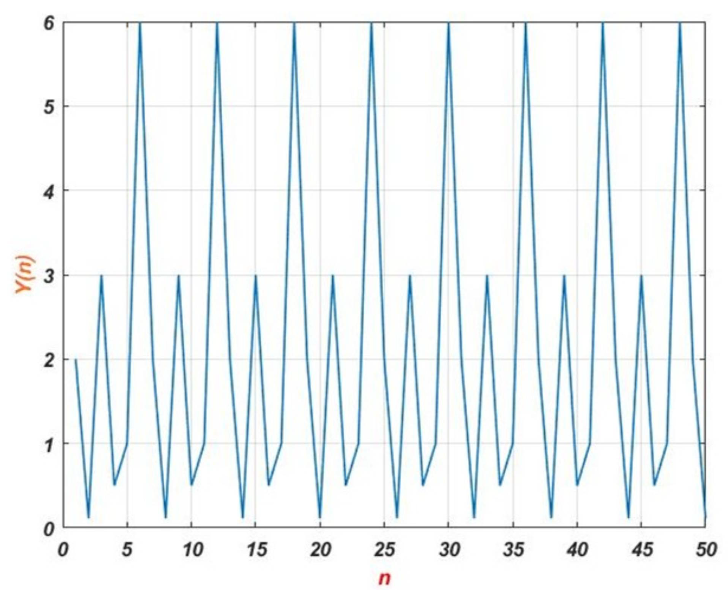
Example 1.

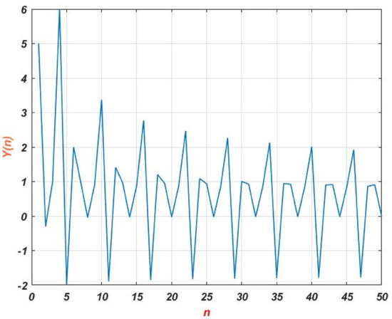
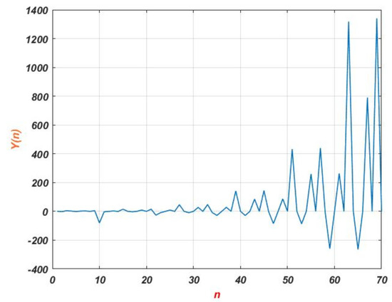
Figure 1 illustrates that the behavior of difference Equation (3) is unstable in response to the random values $Y_{-6}=5$, $Y_{-5}=-0.3$, $Y_{-4}=1$, $Y_{-3}=6$, $Y_{-2}=-2$, $Y_{-1}=2$, and $Y_0=1$.

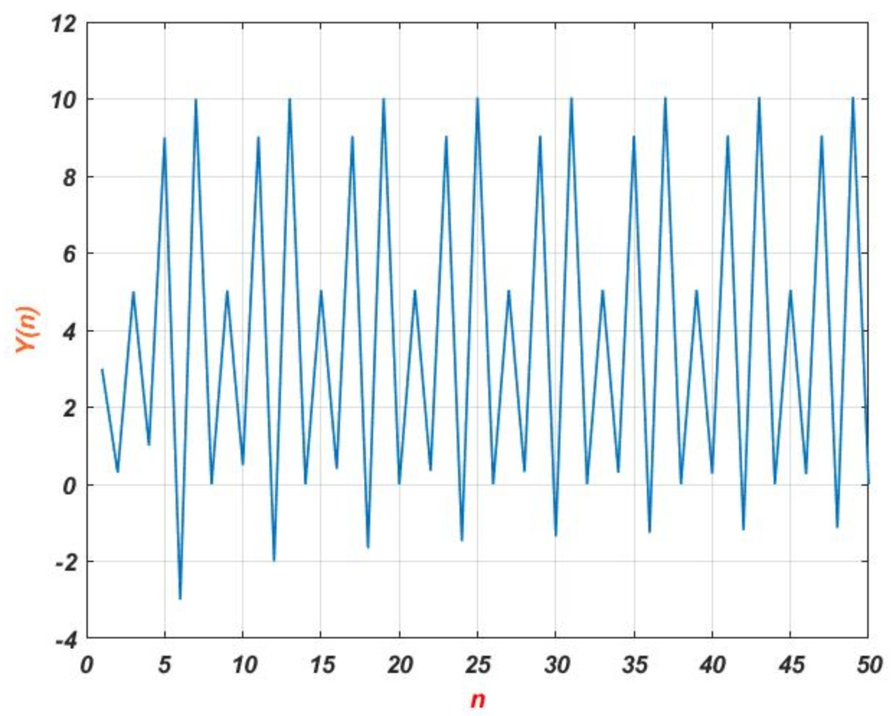
Example 2.

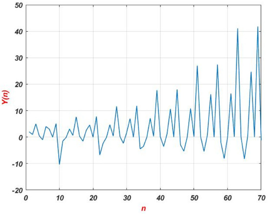
Figure 2 shows that the solution of Equation (8) is unbounded when the initial values are $Y_{-6}=2$, $Y_{-5}=1$, $Y_{-4}=5$, $Y_{-3}=0.5$, $Y_{-2}=-1$, $Y_{-1}=4$, and $Y_0=3$.

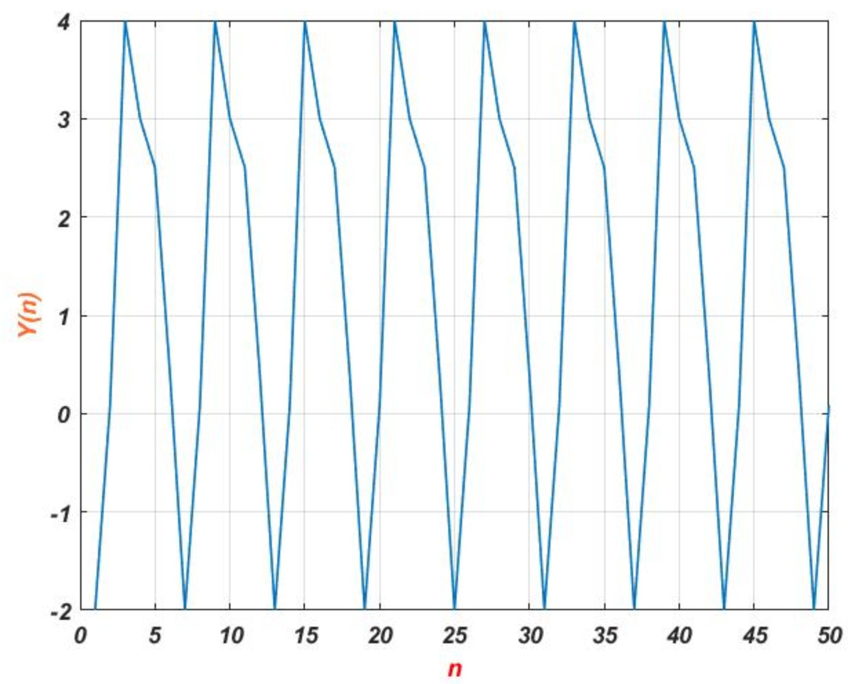
Example 3.

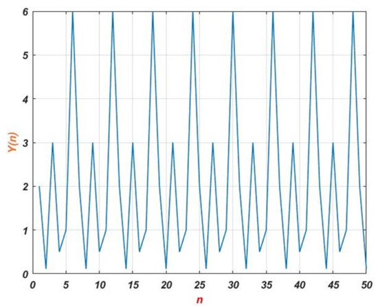
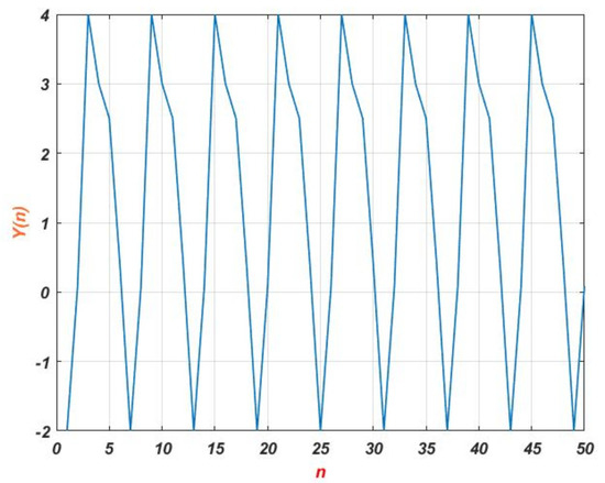
Consider Equation (10) under the initial conditions $Y_{-6}=2$, $Y_{-5}={\displaystyle \frac{1}{9}}$, $Y_{-4}=3$, $Y_{-3}=0.5$, $Y_{-2}=1$, $Y_{-1}=6$, and $Y_0=2$; then, Figure 3 represents a periodic solution of period six.

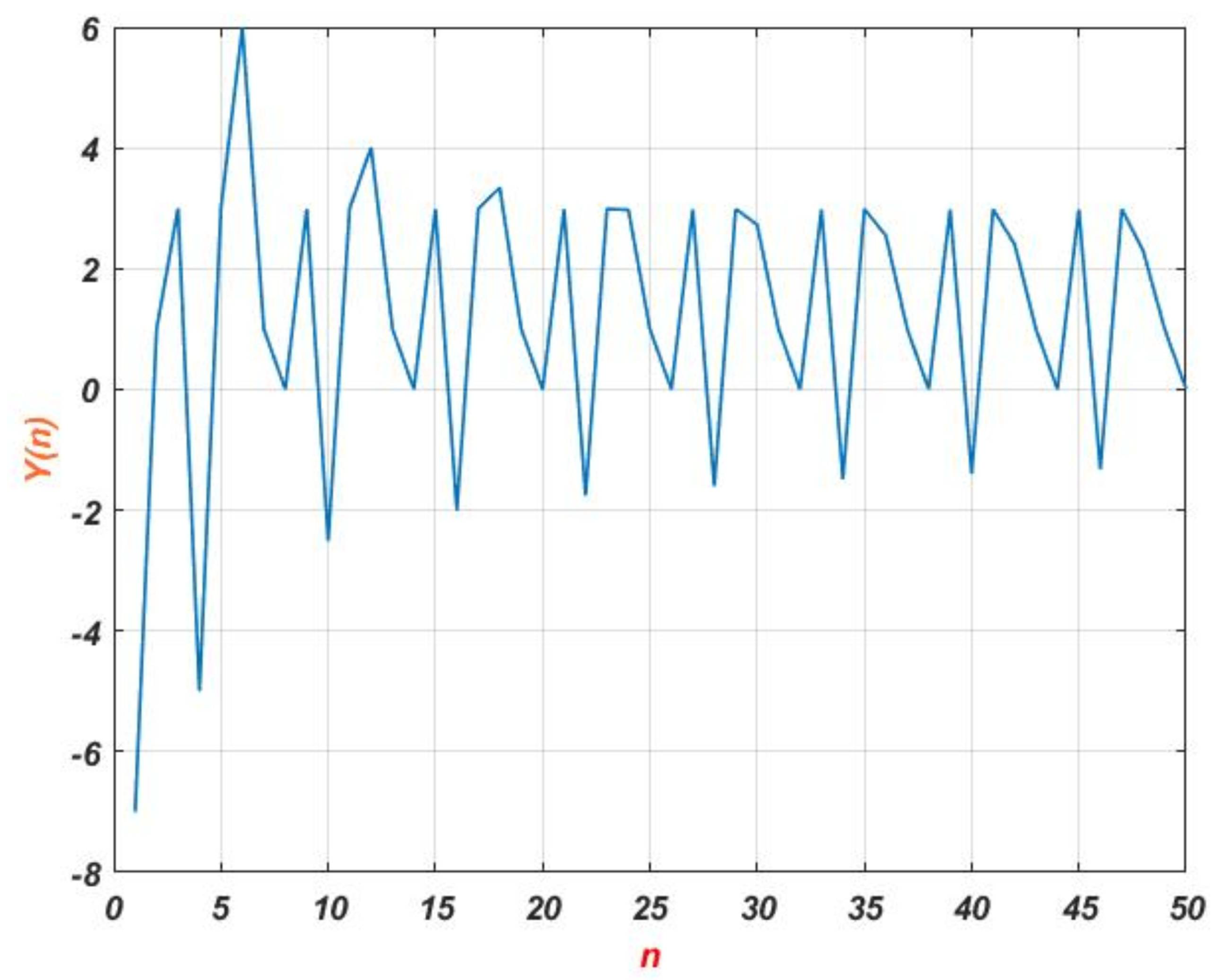
Example 4.

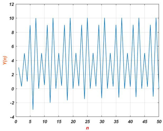
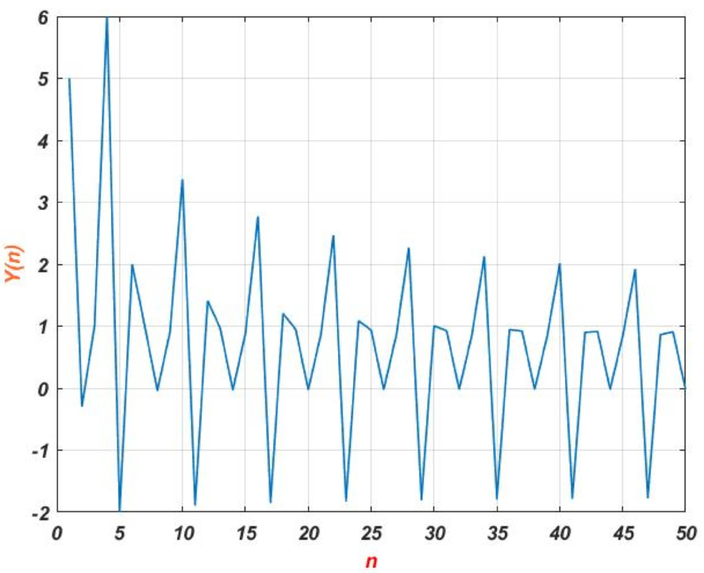
Figure 4 shows the numerical solution of difference Equation (13) with initial values of $Y_{-6}=3$, $Y_{-5}=0.3$, $Y_{-4}=5$, $Y_{-3}=1$, $Y_{-2}=9$, $Y_{-1}=-3$, and $Y_0=10$.

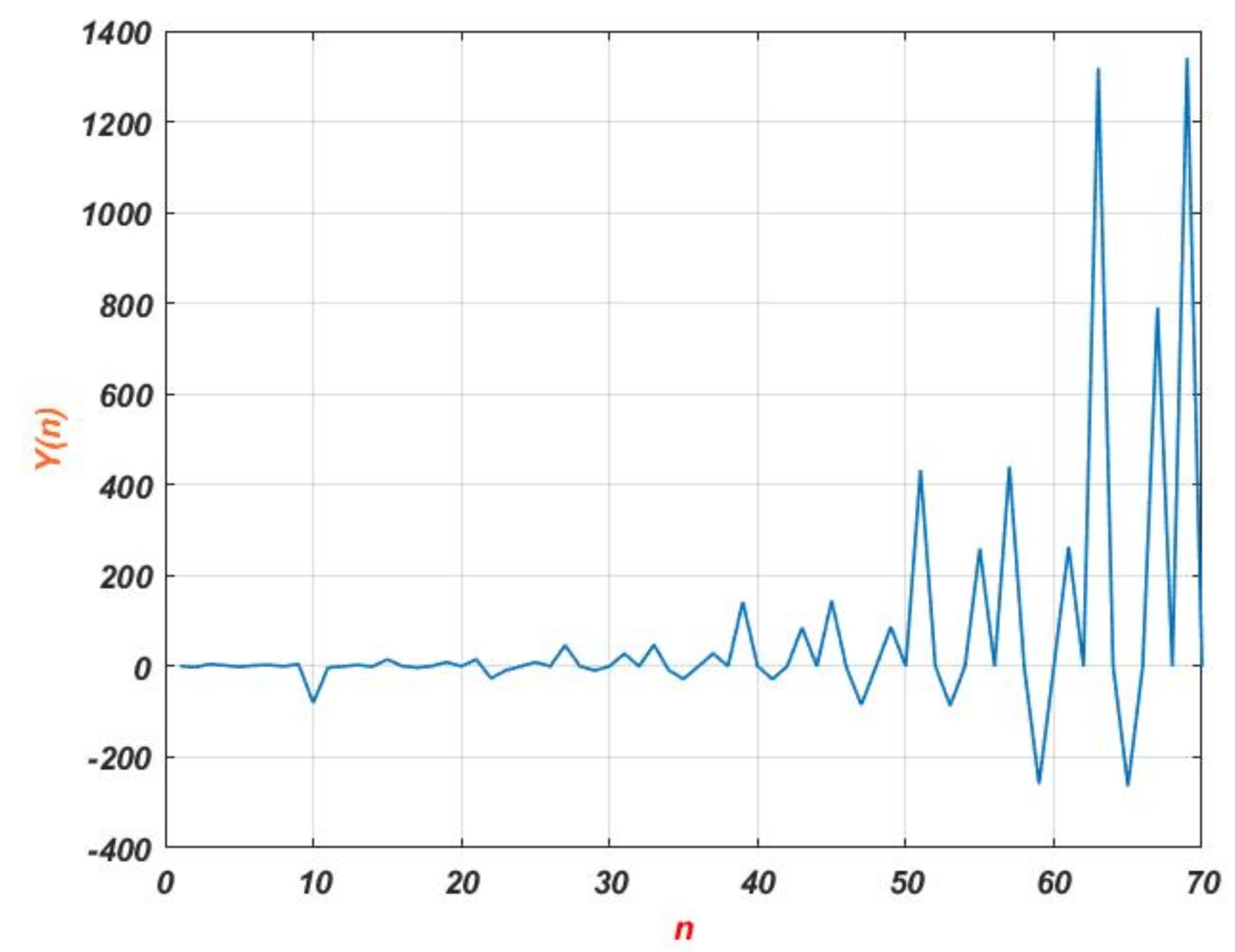
Example 5.

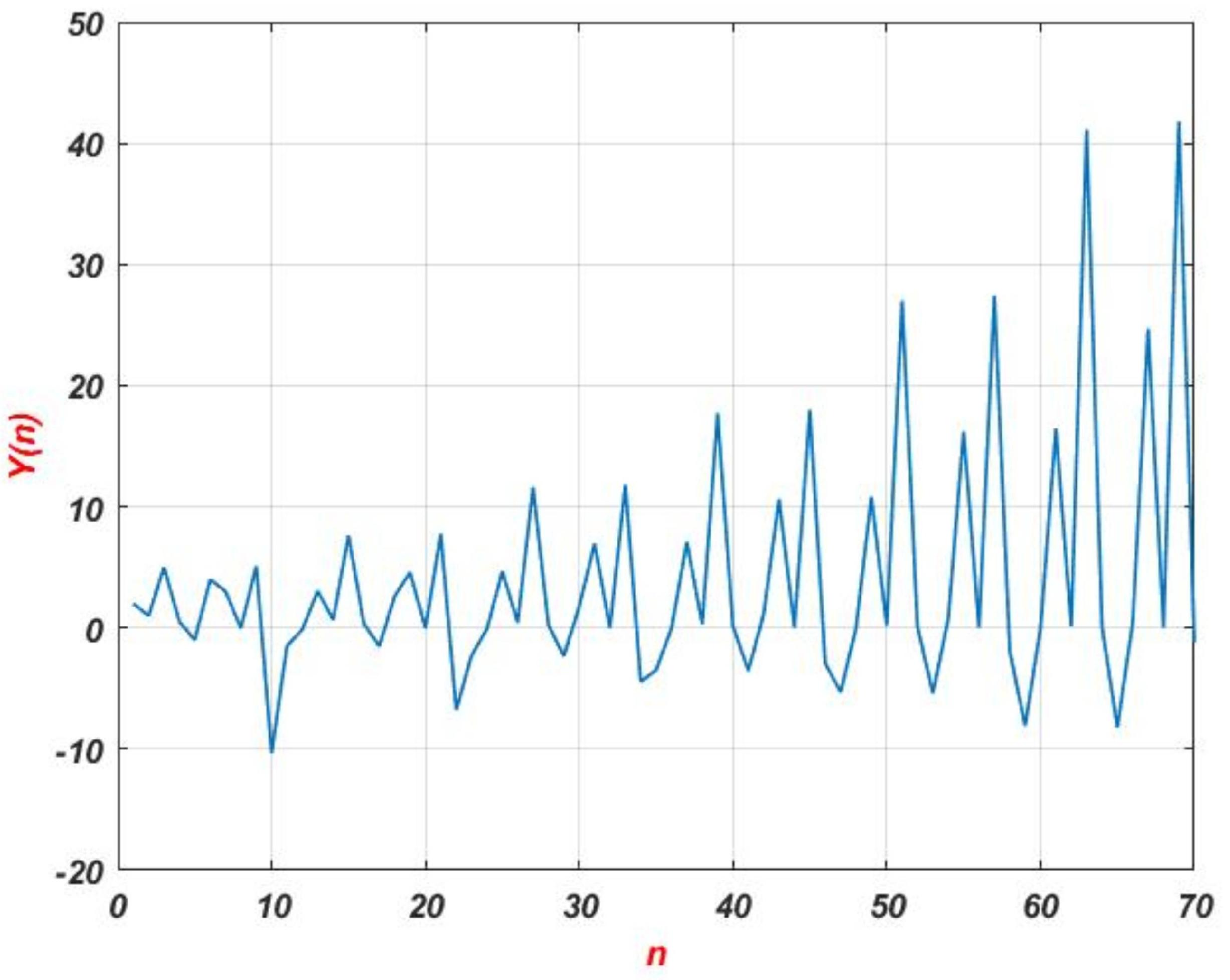
Meanwhile, in Figure 5, the different behavior of solutions for (13) is presented with the following random initial values: $Y_{-6}=-7$, $Y_{-5}=1$, $Y_{-4}=3$, $Y_{-3}=-5$, $Y_{-2}=3$, $Y_{-1}=6$, and $Y_0=1$.

Example 6.

Figure 6 shows the unboundedness solution of Equation (14) when the initial values are $Y_{-6}=1$, $Y_{-5}=-2$, $Y_{-4}=5$, $Y_{-3}=2$, $Y_{-2}=-1$, $Y_{-1}=2$, and $Y_0=3$.

Example 7.

In Figure 7, we show a periodic solution to Equation (14) of period six with the initial values $Y_{-6}=-2$, $Y_{-5}=1/12$, $Y_{-4}=4$, $Y_{-3}=3$, $Y_{-2}=5/2$, $Y_{-1}=2/5$, and $Y_0=-2$.

8. Conclusions

This research examines the solutions and qualitative theory of many higher-order nonlinear difference equations, focusing primarily on their stability, boundedness, and periodicity. Through theoretical methodologies and numerical simulations, we derived explicit solutions for some cases of Equation (1). The results indicate that for these equations, equilibrium points are typically not locally asymptotically stable, leading to chaos, namely, the coexistence of stable unbounded and periodic attractors. Consequently, these findings augment our understanding of nonlinear difference equations, which will be beneficial for their application in mathematical modeling across several scientific disciplines. Future research may focus on applying these methods to other unresolved difference equations and exploring potentially more universal solutions.

References

- Kerker, M.A.; Hadidi, E.; Salmi, A. Qualitative behavior of a higher-order nonautonomous rational difference equation. J. Appl. Math. Comput. 2020, 64, 399–409. [Google Scholar] [CrossRef]
- Almatrafi, M.; Elsayed, E.M.; Alzahrani, F. Investigating Some Properties of a Fourth Order Difference Equation. J. Comput. Anal. Appl. 2019, 28, 243–253. [Google Scholar]
- Garic-Demirovic, M.; Nurkanovic, M.; Nurkanovic, Z. Stability, periodicity and Neimark-Sacker bifurcation of certain homogeneous fractional difference equations. Int. J. Differ. Equations 2017, 12, 27–53. [Google Scholar]
- Tollu, D.T.; Yazlik, Y.; Taskara, N. On a solvable non-inear difference equation of higher order. Turk. J. Math. 2018, 42, 1765–1778. [Google Scholar] [CrossRef]
- El-Metwally, H.; Elsayed, M.E. Qualitative Study of Solutions of Some Difference Equations. Abstr. Appl. Anal. 2012, 16, 248291. [Google Scholar] [CrossRef]
- Jia, L. Dynamic behaviors of a class of high-order fuzzy difference equations. J. Math. 2020, 2020, 1737983. [Google Scholar] [CrossRef]
- Kara, M.; Yazlik, Y.; Tollu, D.T. Solvability of a system of higher order nonlinear difference equations. Hacet. J. Math. Stat. 2020, 49, 1566–1593. [Google Scholar] [CrossRef]
- Ladas, G.; Tzanetopoulos, G.; Tovbis, A. On May’s host parasitoid model. J. Differ. Equations Appl. 1996, 2, 195–204. [Google Scholar] [CrossRef]
- Alayachi, H.S.; Noorani, M.S.; Khan, A.Q.; Almatrafi, M.B. Analytic solutions and stability of sixth order difference equations. Math. Probl. Eng. 2020, 2020, 1230979. [Google Scholar] [CrossRef]
- Ahlbrandt, C.D.; Peterson, A.C. Discrete Hamiltonian Systems: Difference Equations, Continued Fractions, and Riccati Equations; Kluwer Academic Publishers: Amsterdam, The Netherlands, 1996. [Google Scholar]
- Alharbi, T.D.; Elsayed, M.E. Forms of Solution and Qualitative Behavior of Twelfth-Order Rational Difference Equation. Int. J. Differ. Equations 2022, 17, 281–292. [Google Scholar]
- Alharbi, T.D.; Elsayed, M.E. The Solution Expressions and the Periodicity Solutions of Some Nonlinear Discrete Systems. Pan-Amer. J. Math. 2023, 2, 3. [Google Scholar] [CrossRef] [PubMed]
- Alotaibi, A.M.; El-Moneam, M.A. On the dynamics of the nonlinear rational difference equation . AIMS Math. 2022, 7, 7374–7384. [Google Scholar] [CrossRef]
- Beverton, R.J.H.; Holt, S.J. On the Dynamics of Exploited Fish Populations, Fishery Investigations Series II; Blackburn Press: Caldwell, NJ, USA, 2004. [Google Scholar]
- Bektesevic, J.; Mehuljic, M.; Hadziabdic, V. Global Asymptotic Behavior of Some Quadratic Rational Second-Order Difference Equations. Int. J. Differ. Equations 2017, 20, 169–183. [Google Scholar]
- Cull, P.; Flahive, M.; Robson, R. Difference Equations: From Rabbits to Chaos, Undergraduate Texts in Mathematics; Springer: Berlin/Heidelberg, Germany, 2005. [Google Scholar]
- Din, Q.; Elsayed, M.E. Stability analysis of a discrete ecological model. Comput. Ecol. Softw. 2004, 4, 89–103. [Google Scholar]
- Dekkar, I.; Touafek, N.; Din, Q. On the global dynamics of a rational difference equation with periodic coefficients. J. Appl. Math. Comput. 2019, 60, 567–588. [Google Scholar] [CrossRef]
- Elsayed, M.E.; Alharbi, K.N. The expressions and behavior of solutions for nonlinear systems of rational difference equations. J. Innov. Appl. Math. Comput. Sci. (JIAMCS) 2022, 2, 78–91. [Google Scholar]
- Elsayed, M.E.; Alshareef, A. Qualitative Behavior of A System of Second Order Difference Equations. Eur. J. Math. Appl. 2021, 1, 15. [Google Scholar] [CrossRef]
- Elsayed, E.M.; Alofi, B.S.; Khan, A. Qualitative Behavior of Solutions of Tenth-Order Recursive Sequence Equation. Math. Probl. Eng. 2022, 10, 5242325. [Google Scholar] [CrossRef]
- Gümüş, M.; Abo-Zeid, R. Qualitative study of a third order rational system of difference equations. Math. Moravica 2021, 25, 81–97. [Google Scholar] [CrossRef]
- Jana, D.; Elsayed, M.E. Interplay between strong Allee effect, harvesting and hydra effect of a single population discrete—Time system. Int. J. Biomath. 2016, 9, 58–1793. [Google Scholar] [CrossRef]
- Ma, W.X. Global behavior of a higher-order nonlinear difference equation with many arbitrary multivariate functions. East Asian J. Appl. Math. 2019, 9, 643–650. [Google Scholar]
- Moaaz, O.; Chalishajar, C.; Bazighifan, O. Some qualitative behavior of solutions of general class difference equations. Mathematics 2019, 7, 585. [Google Scholar] [CrossRef]
- Murray, J.D. Mathematical Biology: An Introduction; Kluwer Academic Publishers: New York, NY, USA; Springer: Berlin/Heidelberg, Germany, 2002. [Google Scholar]
- Qian, C.; Smith, J. On quasi-periodic solutions of forced higher order nonlinear difference equations. Electron. J. Qual. Theory Differ. Equations 2020, 6, 20. [Google Scholar] [CrossRef]
- Stević, S. On some solvable systems of difference equations. J. Appl. Math. Comput. 2012, 218, 5010–5018. [Google Scholar] [CrossRef]
- Mahmood, B.A.; Yousif, M.A. A novel analytical solution for the modified Kawahara equation using the residual power series method. Nonlinear Dyn. 2017, 89, 1233–1238. [Google Scholar] [CrossRef]
- Yazlik, Y.; Kara, M. On a solvable system of difference equations of higher-order with period two coefficients. Commun. Fac. Sci. Univ. Ank.-Ser.-Math. Stat. 2019, 68, 1675–1693. [Google Scholar] [CrossRef]
- Zayed, E.M.E. On the dynamics of a new nonlinear rational difference. Dyn. Contin. Discret. Impuls. Syst. Math. Anal. 2020, 27, 153–165. [Google Scholar]
- Kulenovic, M.R.S.; Ladas, G. Dynamics of Second Order Rational Difference Equations with Open Problems and Conjectures; Chapman & Hall: New York, NY, USA, 2001. [Google Scholar]
- Kocic, V.L.O.; Ladas, G. Global Behavior of Nonlinear Difference Equations of Higher Order with Applications; Kluwer Academic Publishers: Dordrecht, The Netherlands, 1993. [Google Scholar]
Disclaimer/Publisher’s Note: The statements, opinions and data contained in all publications are solely those of the individual author(s) and contributor(s) and not of MDPI and/or the editor(s). MDPI and/or the editor(s) disclaim responsibility for any injury to people or property resulting from any ideas, methods, instructions or products referred to in the content. |
© 2024 by the authors. Licensee MDPI, Basel, Switzerland. This article is an open access article distributed under the terms and conditions of the Creative Commons Attribution (CC BY) license (https://creativecommons.org/licenses/by/4.0/).