Integral Reinforcement Learning-Based Online Adaptive Dynamic Event-Triggered Control Design in Mixed Zero-Sum Games for Unknown Nonlinear Systems

Abstract

Mixed zero-sum games consider both zero-sum and non-zero-sum differential game problems simultaneously. In this paper, multiplayer mixed zero-sum games (MZSGs) are studied by the means of an integral reinforcement learning (IRL) algorithm under the dynamic event-triggered control (DETC) mechanism for completely unknown nonlinear systems. Firstly, the adaptive dynamic programming (ADP)-based on-policy approach is proposed for solving the MZSG problem for the nonlinear system with multiple players. Secondly, to avoid using dynamic information of the system, a model-free control strategy is developed by utilizing actor–critic neural networks (NNs) for addressing the MZSG problem of unknown systems. On this basis, for the purpose of avoiding wasted communication and computing resources, the dynamic event-triggered mechanism is integrated into the integral reinforcement learning algorithm, in which a dynamic triggering condition is designed to further reduce triggering times. With the help of the Lyapunov stability theorem, the system states and weight values of NNs are proven to be uniformly ultimately bounded (UUB) stable. Finally, two examples are demonstrated to show the effectiveness and feasibility of the developed control method. Compared with static event-triggering mode, the simulation results show that the number of actuator updates in the DETC mechanism has been reduced by 55% and 69%, respectively.

1. Introduction

In recent years, differential games theory has been extensively applied in various fields such as economic and financial decision-making [1,2,3,4], automation control systems [5,6], and computer science [7]. In these studies, multiple participants engaged in continuous games and strove to optimize their respective independent, then conflicting, objectives so the Nash equilibrium could be achieved. In two-player zero-sum games (ZSGs) [8,9], if one player gained, it inevitably resulted in a loss for another player, and precluded any possibility of cooperation. However, in multi-person non-zero-sum games (NZSGs) [7,10], the total sum of benefits or losses for the parties involved were not zero, thus they allowed for the possibility of a win–win scenario and subsequent cooperation. Based on the characteristics and advantages of these two types of games, Ref. [11] proposed a novel game strategy distinct from ZSGs and NZSGs, termed MZSGs. In such scenarios, determining the Nash equilibrium typically involved solving the coupled Hamilton–Jacobi–Bellman (HJB) equations. When the system was linear, the solution could be obtained by simplifying the HJ equations to algebraic Riccati equations. However, when the system was nonlinear, obtaining analytical solutions became challenging due to the presence of coupling terms in the equations.

To address the issue of unattainable analytical solutions, researchers devised a novel method based on the ADP algorithm to approximate optimal solutions [12,13,14,15]. This method was applied in numerous control domains to tackle various problems, such as $H_{\infty }$ control issues [16], time-delay system control [17], optimal spin polarization control [18], and reinforcement learning (RL) control [19]. In the work of [18], a new ADP structure was proposed for three-dimensional spin polarization control. A novel ADP method, entirely independent of system information, was introduced for nonlinear Markov jump systems in order to solve the two-player Stackelberg differential game in [20]. In the work of [21], an iterative ADP algorithm was proposed to iteratively solve the parameterized Bellman equation for the global stabilization of continuous-time linear systems under control constraints.

The integral reinforcement learning (IRL) algorithm was proposed as a derivative of the RL algorithm in [22]. In policy iteration-based ADP algorithms, an approximate optimal solution to the HJB equation was required. However, in the IRL algorithm, model-free implementation was achievable, which means that the HJB equation could be solved without any knowledge of system dynamics [23]. Due to the difficulty in modeling or accurately describing system dynamics in practical problems, the IRL algorithm has been widely applied to address optimal control problems. In [24], it was demonstrated that data-based IRL algorithms were equivalent to model-based policy iteration algorithms. Researchers utilized the IRL algorithm to obtain iterative control, thereby achieving policy evaluation and policy improvement [25]. Moreover, a novel guaranteed cost control was designed using the IRL algorithm, which aimed to relax the system dynamics knowledge of stochastic systems modulated by stochastic time-varying parameters in [26]. In the research by [27], an adaptive optimal bipartite consensus scheme was developed using the IRL algorithm in order to contribute a critic-only controller structure. However, these control methods had all been developed on the basis of a time-triggered mechanism; the defining characteristic of the mechanism was that the sampled data and each control update were periodic. However, as systems gradually stabilized or operated within permissible performance margins, it became desirable for controllers to remain in a static state [28].

In response to these requirements, researchers proposed static event-triggered control (SETC) for sampling processes, which can ensure stable system operation. Specifically, a novel triggering condition was pre-designed by the authors, which mapped to a defined threshold. The controller would only update when this condition was met, significantly reducing the wastage of communication resources [29,30,31,32]. Nevertheless, the triggering rules associated with static event triggers were solely dependent on the current state and error signals and disregarded previous values. This limitation was addressed in Girard’s research in [33], where an internal dynamic variable was incorporated into the previous triggering mechanism. This enhancement made the triggering mechanism contingent not only related to current values but also associated historical data, which led to the development of DETC. The advantage of this new mechanism laid in its ability to extend the interval between triggers. In subsequent studies [34,35,36,37], researchers extensively explored the application of DETC in multi-agent systems, theoretically proving their feasibility. Ref. [38] investigated fault-tolerant control issues based on DETC, where the dynamic variable adopted a form more general than exponential functions. Ref. [39] investigated non-fragile dissipative filters for discrete-time interval type-2 fuzzy Markov jump systems.

In this paper, an online algorithm was proposed based on ADP to address the IRL online adaptive DETC problem for MZSGs with unknown nonlinear systems. The main contributions are given as follows:

1.

Unlike the studies on ZSG or NZSG problems in [8,19,24,30], the ZSG and NZSG problems are considered simultaneously, in which an event-triggered ADP approach is used to solve the problem to reduce communication and computing resources.

2.

By establishing the actor NNs to approximate the optimal control strategies and auxiliary control inputs of each player, a novel event-triggered IRL algorithm is proposed to solve the mixed zero-sum games problem without using the information of system functions.

3.

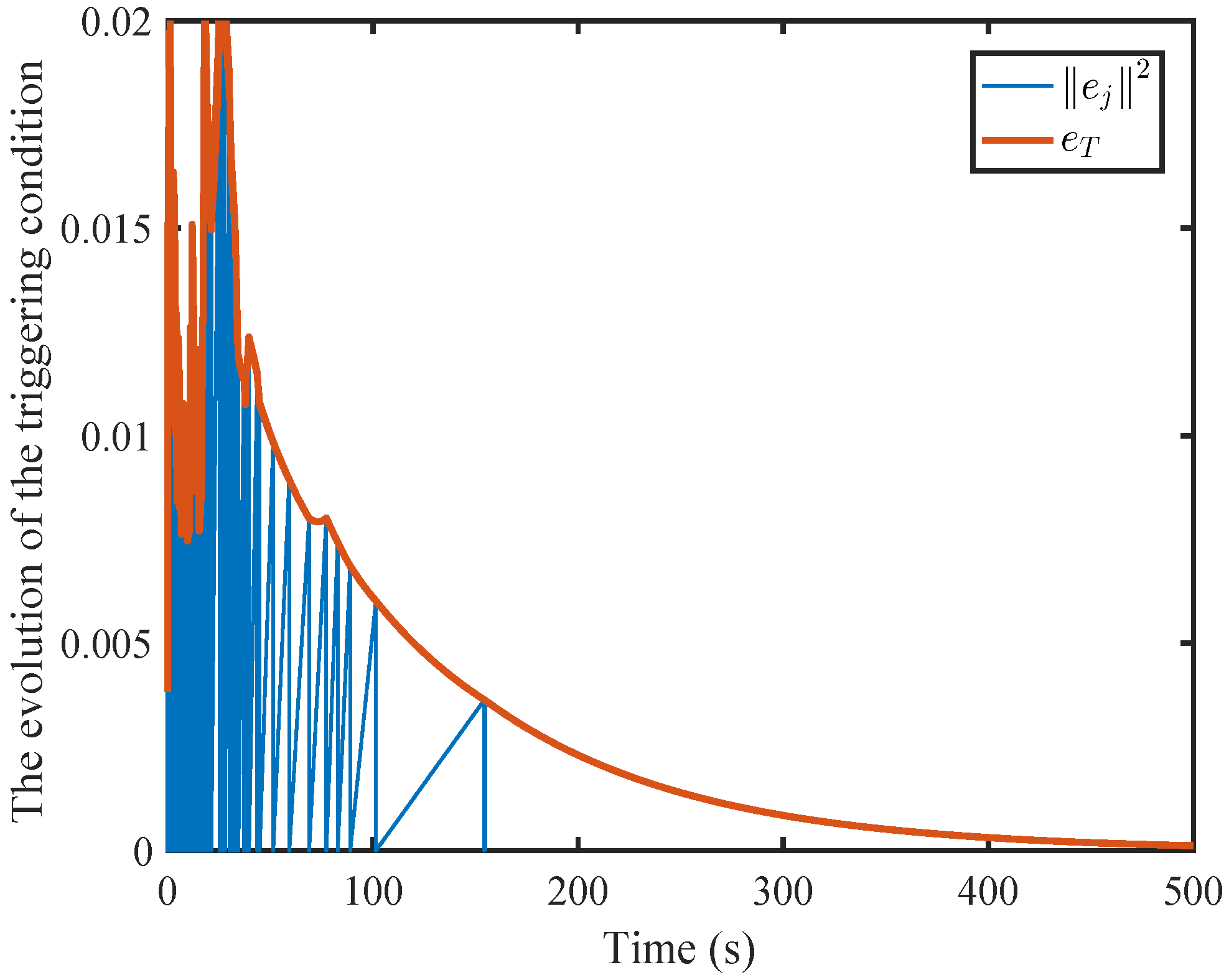
In the developed off-policy DETC method, by introducing the dynamic adaptive parameters to the triggering conditions, compared with the static event-triggered mechanism, the triggering frequency is further reduced, thereby achieving greater utilization of communication resources.

The rest of this paper is organized as follows. Section 2, elaborates on unknown nonlinear systems and introduces knowledge of multiplayer MZSGs. Section 3 proposes ADP-based near-optimal control for MZSGs under the DETC mechanism. Section 4 develops a dynamic event-triggered IRL algorithm for unknown systems. Section 5 proves the UUB properties of closed-loop system states and the convergence of critical NN weight estimation errors. Section 6 provides two example results to validate the effectiveness of the developed algorithms. Finally, Section 7 presents the conclusion of this paper.

2. Problem Formulation

Consider the following multiplayer games system

$$\begin{array}{c}\hfill \dot{\vartheta }=f\left(\vartheta \right)+\sum _{j=1}^{N+1}{h}_j\left(\vartheta \right)v_j,\end{array}$$

(1)

where $\vartheta \in {\Re }^n$ is the system state, $f\left(\vartheta \right)\in {\Re }^n$ and $h_j\left(\vartheta \right)\in {\Re }^{n\times m_j}$ are unknown system and control dynamics, $v_j\in {\mathbb{R}}^{m_j}$ are the control inputs, and $\vartheta \left(0\right)={\vartheta }_0$ is the initial system state.

Assumption 1.

$f\left(0\right)=0,f\left(\vartheta \right)\le {\mathbb{B}}_f∥\vartheta ∥$, ${\mathbb{B}}_f$ is a positive constant. $f\left(\vartheta \right)$ and $h_i\left(\vartheta \right)$ are Lipschitz continuous on a compact set $\Omega \subseteq R^n$, which contains the origin, and the system is stable.

For system (1), these $N+1$ participants exhibit varying competitive dynamics, where the first N participants engage in cooperative relationships akin to NZSGs, and the N-th and ($N+1$)-th participants engage in competitive interactions akin to ZSGs. We can identify equilibrium strategies that stabilize the system, defining the cost function of the i-th participant based on their interactions with others

$$\begin{array}{cc}\hfill J_i\left(\vartheta \right)& ={\int }_0^{\infty }({\vartheta }^T{B}_i\vartheta +\sum _{j=1}^N{v}_j^T{R}_{i,j}{v}_j)ds,i\in {\rm Y},i\ne N,\hfill \end{array}$$

(2)

$$\begin{array}{cc}\hfill J_N\left(\vartheta \right)& ={\int }_0^{\infty }({\vartheta }^T{B}_N\vartheta +\sum _{j=1}^N{v}_j^T{R}_{N,j}{v}_j-{\gamma }^2∥v_{N+1}∥)ds,\hfill \end{array}$$

(3)

where ${\rm Y}=\left\{1,2,\dots ,N\right\}$, $B_i\ge 0,R_{i,j}>0$ and $\gamma$ is a positive constant.

Definition 1.

There is a series of control policy $v=\left\{v_1,\dots ,v_N,v_{N+1}\right\}$ which is continuous on Ω, when the system (1) is stable and the cost functions (2) and (3) are finite over Ω. It is considered as admissible, denoted by $v\in \Theta (\Omega )$.

The value functions corresponding to (4) and (5) are

$$\begin{array}{cc}\hfill Q_i^{*}\left(\vartheta \right)& =\underset{v_i\in \Theta \left(\Omega \right)}{min}{\int }_t^{\infty }({\vartheta }^T{B}_i\vartheta +\sum _{j=1}^N{v}_j^T{R}_{i,j}{v}_j)ds,\hfill \end{array}$$

(4)

$$\begin{array}{cc}\hfill Q_N^{*}\left(\vartheta \right)& =\underset{v_N\in \Theta \left(\Omega \right)}{min}\underset{v_{N+1}\in \Theta \left(\Omega \right)}{max}{\int }_t^{\infty }({\vartheta }^T{B}_N\vartheta +\sum _{j=1}^N{v}_j^T{R}_{N,j}{v}_j\hfill \\ \hfill & -{\gamma }^2{v}_{N+1}^T{v}_{N+1})ds,\hfill \end{array}$$

(5)

where $i\in {\rm Y},i\ne N$. Let ${\vartheta }^T{B}_i\vartheta +{\sum }_{j=1}^N{v}_j^T{R}_{i,j}{v}_j$ = $r_i$, $i\ne N$ and ${\vartheta }^T{B}_N\vartheta +{\sum }_{j=1}^N{v}_j^T{R}_{N,j}{v}_j-{\gamma }^2{v}_{N+1}^T{v}_{N+1}$ = $r_N$. Our intention is to find the optimal control inputs $v^{*}=\left\{v_1^{*},\dots ,v_N^{*},v_{N+1}^{*}\right\}$.

  If the optimal value functions (2) and (3) are differentiable on $\Omega$, the Hamilton functions are defined as

$$\begin{array}{cc}\hfill & H_i\left(\vartheta ,\nabla Q_i,v_1,\dots ,v_N,v_{N+1}\right)\hfill \\ \hfill =& r_i\left(\vartheta ,v_1,\dots ,v_N\right)+{\left(\nabla Q_i\right)}^T\left(f\left(\vartheta \right)+\sum _{j=1}^{N+1}{h}_j\left(\vartheta \right)v_j\right),i\in {\rm Y},i\ne N,\hfill \end{array}$$

(6)

$$\begin{array}{cc}\hfill & H_N\left(\vartheta ,\nabla Q_N,v_1,\dots ,v_N,v_{N+1}\right)\hfill \\ \hfill =& r_N\left(\vartheta ,v_1,\dots ,v_N,v_{N+1}\right)+{\left(\nabla Q_N\right)}^T\left(f\left(\vartheta \right)+\sum _{j=1}^{N+1}{h}_j\left(\vartheta \right)v_j\right),\hfill \end{array}$$

(7)

where $\nabla Q_i=\partial Q_i/\partial \vartheta ,i\in N$. HJ functions are determined by

$$\begin{array}{c}\hfill H_i\left(\vartheta ,\nabla Q_i,v_1,\dots ,v_N,v_{N+1}\right)=0,i\in {\rm Y}.\end{array}$$

(8)

At equilibrium, there exist $N+1$ stability conditions

$$\begin{array}{c}\hfill {\displaystyle \frac{\partial H_i}{\partial v_i}}=0,{\displaystyle \frac{\partial H_N}{\partial v_{N+1}}}=0,i\in {\rm Y}.\end{array}$$

(9)

Next, using stationary conditions, we can obtain

$$\begin{array}{cc}\hfill v_i^{*}\left(\vartheta \right)& =-{\displaystyle \frac{1}{2}}{R}_{i,i}^{-1}{h}_i^T{\displaystyle \frac{\partial Q_i^{*}}{\partial \vartheta }},i\in {\rm Y},\hfill \end{array}$$

(10)

$$\begin{array}{cc}\hfill v_{N+1}^{*}\left(\vartheta \right)& ={\displaystyle \frac{1}{2{\gamma }^2}}{h}_{N+1}^T{\displaystyle \frac{\partial Q_N^{*}}{\partial \vartheta }}.\hfill \end{array}$$

(11)

Remark 1.

From (10) and (11), it follows that if (8) has a unique solution, then N + 1 participants possess optimal control. γ is a parameter ensuring the unique solution of the MZSGs. According to [39], when γ exceeds ${\gamma }^{*}$, the HJB equation admits a unique solution, thus ${\gamma }^{*}$ denotes a threshold.

Substituting the optimal control strategies Equations (10) and (11) into (8), the coupled HJ equation under time-triggered conditions can be obtained by

$$\begin{array}{cc}\hfill & {\vartheta }^T{B}_i\vartheta +{\left(\nabla Q_i^{*}\right)}^T\left(f\left(\vartheta \right)-{\displaystyle \frac{1}{2}}\sum _{j=1}^N{h}_j{R}_{j,j}^{-1}{h}_j^T\nabla Q_j^{*}+{\displaystyle \frac{1}{2{\gamma }^2}}{h}_{N+1}{h}_{N+1}^T\nabla Q_N^{*}\right)\hfill \\ \hfill & +{\displaystyle \frac{1}{4}}\sum _{j=1}^N{\left(\nabla Q_j^{*}\right)}^T{h}_j{R}_{j,j}^{-1}{R}_{i,j}{R}_{j,j}^{-1}{h}_j^T\nabla Q_j^{*}=0,i\in {\rm Y},i\ne N,\hfill \end{array}$$

(12)

$$\begin{array}{cc}\hfill & {\vartheta }^T{B}_N\vartheta +{\displaystyle \frac{1}{4}}\sum _{j=1}^N{\left(\nabla Q_j^{*}\right)}^T{h}_j{R}_{j,j}^{-1}{R}_{N,j}{R}_{j,j}^{-1}{h}_j^T\nabla Q_j^{*}\hfill \\ \hfill & -{\displaystyle \frac{1}{4{\gamma }^2}}{\left(\nabla Q_N^{*}\right)}^T{h}_{N+1}{h}_{N+1}^T\nabla Q_N^{*}\hfill \\ \hfill & +{\left(\nabla Q_N\right)}^T\left(f\left(\vartheta \right)-{\displaystyle \frac{1}{2}}\sum _{j=1}^N{h}_j{R}_{j,j}^{-1}{h}_j^T\nabla Q_j^{*}+{\displaystyle \frac{1}{2{\gamma }^2}}{h}_{N+1}{h}_{N+1}^T\nabla Q_N^{*}\right)=0.\hfill \end{array}$$

(13)

3. ADP-Based Near-Optimal Control for MZSGs Under DETC Mechanism

The dynamic event-triggered mechanism put in this paper represents $\left\{t_k\right\}$ as a singular monotonically increasing sequence of trigger instants, which satisfies that the condition $0=t_0<t_1<\cdots <t_k<\cdots$. ${\overline{\vartheta }}_k\left(t\right)=\vartheta \left(t_k\right)$ is denoted as the state at trigger time $t_k$, and the event-triggered errors are defined as:

$$\begin{array}{c}\hfill e_{k,i}=\vartheta \left(t\right)-{\overline{\vartheta }}_k\left(t\right),t_k\le t\le t_{k+1}.\end{array}$$

(14)

Recalling (10) and (11), the event-triggered optimal control policies are obtained as

$$\begin{array}{cc}\hfill {\overline{v}}_i^{*}\left({\overline{\vartheta }}_k\right)& =-{\displaystyle \frac{1}{2}}{R}_{i,i}^{-1}{h}_i^T\left({\overline{\vartheta }}_k\right)\nabla {\overline{Q}}_i^{*}\left({\overline{\vartheta }}_k\right),i\in {\rm Y},\hfill \end{array}$$

(15)

$$\begin{array}{cc}\hfill {\overline{v}}_{N+1}^{*}\left({\overline{\vartheta }}_k\right)& ={\displaystyle \frac{1}{2{\gamma }^2}}{h}_{N+1}^T\left({\overline{\vartheta }}_k\right)\nabla {\overline{Q}}_N^{*}\left({\overline{\vartheta }}_k\right),\hfill \end{array}$$

(16)

where $\nabla {\overline{Q}}_i^{*}={\displaystyle \frac{\partial Q_i^{*}}{\partial x}}{\mid }_{t=t_k}$ with $i\in \Gamma$. By substituting (15) and (16), the event-triggered HJ equations are represented as:

$$\begin{array}{c}{H}_i\left(\vartheta ,\nabla Q_i^{*},{\overline{v}}_1^{*},\dots ,{\overline{v}}_N^{*},{\overline{v}}_{N+1}^{*}\right)\hfill \\ ={\vartheta }^T{B}_i\vartheta +{\displaystyle \frac{1}{4}}\sum _{j=1}^N{\left(\nabla {\overline{Q}}_j^{*}\left({\overline{\vartheta }}_k\right)\right)}^T{h}_j\left({\overline{\vartheta }}_k\right)R_{j,j}^{-1}{R}_{i,j}{R}_{j,j}^{-1}{h}_j^T\left({\overline{\vartheta }}_k\right)\nabla {\overline{Q}}_j^{*}\left({\overline{\vartheta }}_k\right)\hfill \\ +{\left(\nabla Q_i^{*}\right)}^T\left(f\left(\vartheta \right)-{\displaystyle \frac{1}{2}}\sum _{j=1}^N{h}_j{R}_{j,j}^{-1}{h}_j\left({\overline{\vartheta }}_k\right)\nabla {\overline{Q}}_j^{*}\left({\overline{\vartheta }}_k\right)\right.\hfill \\ \left.+{\displaystyle \frac{1}{2{\gamma }^2}}{h}_{N+1}{h}_{N+1}^T\left({\overline{\vartheta }}_k\right)\nabla {\overline{Q}}_N^{*}\left({\overline{\vartheta }}_k\right)\right),\hfill \end{array}$$

(17)

$$\begin{array}{cc}\hfill & H_N\left(\vartheta ,\nabla Q_N^{*},{\overline{v}}_1^{*},\dots ,{\overline{v}}_N^{*},{\overline{v}}_{N+1}^{*}\right)\hfill \\ \hfill & ={\vartheta }^T{B}_N\vartheta +{\displaystyle \frac{1}{4}}\sum _{j=1}^N{\left(\nabla {\overline{Q}}_j^{*}\left({\overline{\vartheta }}_k\right)\right)}^T{h}_j\left({\overline{\vartheta }}_k\right)R_{j,j}^{-1}{R}_{N,j}{R}_{j,j}^{-1}{h}_j{\left({\overline{\vartheta }}_k\right)}^T\nabla {\overline{Q}}_j^{*}\left({\overline{\vartheta }}_k\right)\hfill \\ \hfill & -{\displaystyle \frac{1}{4{\gamma }^2}}{\left(\nabla {\overline{Q}}_i^{*}\left({\overline{\vartheta }}_k\right)\right)}^T{h}_{N+1}\left({\overline{\vartheta }}_k\right)h_{N+1}^T\left({\overline{\vartheta }}_k\right)\nabla {\overline{Q}}_i^{*}\left({\overline{\vartheta }}_k\right)\hfill \\ \hfill & +{\left(\nabla Q_N^{*}\right)}^T\left(f\left(\vartheta \right)-{\displaystyle \frac{1}{2}}\sum _{j=1}^N{h}_j{R}_{j,j}^{-1}{h}_j^T\left({\overline{\vartheta }}_k\right)\nabla {\overline{Q}}_j^{*}\left({\overline{\vartheta }}_k\right)\right.\hfill \\ \hfill & \left.+{\displaystyle \frac{1}{2{\gamma }^2}}{h}_{N+1}{h}_{N+1}^T\left({\overline{\vartheta }}_k\right)\nabla {\overline{Q}}_N^{*}\left({\overline{\vartheta }}_k\right)\right).\hfill \end{array}$$

(18)

Assumption 2.

All optimal control policies $v_i^{*}$ exhibit local Lipschitz continuity concerning the event-triggered error $e_{k,i}$. That is, with $\forall i\in {\rm Y}$, $k\in {\mathbb{N}}^{+}$ and $t_k\le t\le t_{k+1}$, we can always find a normal number $L_u>0$ that makes $∥v_i^{*}-{\overline{v}}_i^{*}∥\le L_u∥e_{k,i}∥$ hold.

Theorem 1.

Considering system (1), assume that Assumptions 1 and 2 hold and the value of cost performance is finite. The feedback control policies (10) and (11) from (8) are the equilibrium strategy, and a new dynamic triggering condition is applied as

$$\begin{array}{c}\hfill {∥e_{k,i}\left(\vartheta \right)∥}^2\le {\displaystyle \frac{4{\sum }_{i=1}^N{\beta }_i{\omega }_i+\sigma {\lambda }_{min}\left(B\right){∥\vartheta ∥}^2-4{\gamma }^2{∥{\overline{v}}_{N,N+1}^{*}\left({\overline{\vartheta }}_k\right)∥}^2}{4{\lambda }_{max}\left(\Xi \right)\left(N+1\right)L_u^2}},\end{array}$$

(19)

where ${\beta }_i>0$ and internal signal ${\omega }_i$ are defined as

$$\begin{array}{c}\hfill {\dot{\omega }}_i=-{\beta }_i{\omega }_i+{\displaystyle \frac{1}{4N}}\sigma {\lambda }_{min}\left(B\right){∥\vartheta ∥}^2.\end{array}$$

(20)

When this triggering condition is violated, the optimal control policies (15) and (16) under the dynamic event-triggering pattern can make system (1) UUB stable. The tuning parameters $\sigma \in \left[0,1\right)$ can be chosen by the designer, with Ξ and B as defined in the following (23).

Proof. 

The Lyapunov function is $L={\nu }_1+{\nu }_2={\sum }_{i=1}^N{Q}_i^{*}\left(\vartheta \left(t\right)\right)+{\sum }_{i=1}^N{\omega }_i$, where ${\nu }_1={\sum }_{i=1}^N{Q}_i^{*}\left(\vartheta \left(t\right)\right)$ and ${\nu }_2={\sum }_{i=1}^N{\omega }_i$.

  When implementing the optimal control policies (15) and (16) under the DETC method, the derivative of ${\nu }_1$ along the trajectory of system (1) is

$$\begin{array}{c}\hfill {\dot{\nu }}_1=\sum _{i=1}^N{\left(\nabla Q_i^{*}\right)}^T\left(f\left(\vartheta \right)+\sum _{j=1}^{N+1}{h}_j{\overline{v}}_j^{*}\left({\overline{\vartheta }}_k\right)\right).\end{array}$$

(21)

According to the coupled HJB equations (12) and (13), we have

$$\begin{array}{cc}\hfill & \sum _{i=1}^N{\left(\nabla Q_i^{*}\right)}^{T}f\left(\vartheta \right)\hfill \\ \hfill =& -\sum _{i=1}^N\left({\vartheta }^T{B}_i\vartheta +\sum _{j=1}^N{\left(v_j^{*}\right)}^T{R}_{i,j}{v}_j^{*}+{\left(\nabla Q_i^{*}\right)}^T\sum _{j=1}^{N+1}{h}_j\left(\vartheta \right)v_j^{*}\right)\hfill \\ \hfill & +{\gamma }^2{v}_{N,N+1}^{*T}{v}_{N,N+1}^{*}.\hfill \end{array}$$

(22)

The augmented optimal control signal can be indicated by $v^{*}={\left[v_1^{*T},\dots ,v_N^{*T}\right]}^T$ and the augmented control error can be indicated by ${\breve{v}}^{*}={\left[{\left({\overline{v}}_1^{*}-v_1^{*}\right)}^T,\dots ,{\left({\overline{v}}_N^{*}-v_N^{*}\right)}^T\right]}^T$. Substituting (22) into (21) yields:

$$\begin{array}{cc}\hfill {\dot{\nu }}_1& =-\sum _{i=1}^N{\vartheta }^T{B}_i\vartheta -\sum _{i=1}^N\sum _{j=1}^N{v}_j^{*T}{R}_{i,j}{v}_j^{*}\hfill \\ \hfill & -\sum _{i=1}^N{\left(\nabla Q_i^{*}\right)}^T\sum _{j=1}^{N+1}{h}_j\left(\vartheta \right)\left(v_j^{*}-{\overline{v}}_j^{*}\right)+{\gamma }^2{v}_{N,N+1}^{*T}{v}_{N,N+1}^{*}\hfill \\ \hfill & =-{\vartheta }^{T}B\vartheta -v^{*T}R{v}^{*}-2v^{*T}Y{\overline{v}}^{*}+{\gamma }^2{v}_{N,N+1}^{*T}{v}_{N,N+1}^{*}\hfill \\ \hfill & \le -{\vartheta }^{T}B\vartheta -v^{*T}R{v}^{*}+v^{*T}R{v}^{*}\hfill \\ \hfill & +{\breve{v}}^{*T}{Y}^T{R}^{-1}Y{\breve{v}}^{*}+{\gamma }^2{∥{\overline{v}}_{N,N+1}^{*}\left({\overline{\vartheta }}_k\right)∥}^2\hfill \\ \hfill & =-{\vartheta }^{T}B\vartheta +{\breve{v}}^{*T}\Xi {\breve{v}}^{*}+{\gamma }^2{∥{\overline{v}}_{N,N+1}^{*}\left({\overline{\vartheta }}_k\right)∥}^2,\hfill \end{array}$$

(23)

where $B={\sum }_{i=1}^N{B}_i$, $R=diag\left\{{\sum }_{i=1}^N{R}_{i,1},\dots ,{\sum }_{i=1}^N{R}_{i,N}\right\}$, $\Xi =Y^T{R}^{-1}Y$ and

$Y=\left[\begin{array}{cccc}{R}_{1,1}{h}_1^{-P}{h}_1& R_{1,1}{h}_1^{-P}{h}_2& \cdots & R_{1,1}{h}_1^{-P}{h}_{N+1}\\ ⋮& & & ⋮\\ R_{N,N}{h}_N^{-P}{h}_1& R_{N,N}{h}_N^{-P}{h}_2& \cdots & R_{N,N}{h}_N^{-P}{h}_{N+1}\end{array}\right]$. $h_i^{-P}$ is the pseudo-inverse of $h_i$.

  It can be observed that B, R, and $R^{-1}$ are all positive definite, thus the eigenvalues of $\Xi$ are greater than zero. Because Y is not a zero matrix, both the smallest eigenvalue of B and the largest eigenvalue of $\Xi$ are greater than zero; then, we have

$$\begin{array}{cc}\hfill {\dot{\nu }}_1& \le -\left(1-{\displaystyle \frac{1}{2}}\sigma \right){\vartheta }^{T}B\vartheta -{\displaystyle \frac{1}{2}}\sigma {\lambda }_{min}\left(B\right){∥\vartheta ∥}^2\hfill \\ \hfill & +{\lambda }_{max}\left(\Xi \right)\sum _{j=1}^{N+1}{∥{\overline{v}}_j^{*}-v_j^{*}∥}^2+{\gamma }^2∥{\overline{v}}_{N,N+1}^{*}\left({\overline{\vartheta }}_k\right)∥\hfill \\ \hfill & \le -\left(1-{\displaystyle \frac{1}{2}}\sigma \right){\vartheta }^{T}B\vartheta -{\displaystyle \frac{1}{2}}\sigma {\lambda }_{min}\left(B\right){∥\vartheta ∥}^2\hfill \\ \hfill & +{\lambda }_{max}\left(\Xi \right)\left(N+1\right)L_u^2{∥e_{k,i}∥}^2+{\gamma }^2∥{\overline{v}}_{N,N+1}^{*}\left({\overline{\vartheta }}_k\right)∥.\hfill \end{array}$$

(24)

On the other hand (20), we have

$$\begin{array}{c}\hfill {\dot{\nu }}_2\le -\sum _{i=1}^N{\beta }_i{\omega }_i+{\displaystyle \frac{1}{4}}\sigma {\lambda }_{min}\left(B\right){∥\vartheta ∥}^2.\end{array}$$

(25)

Combining (24) and (25), it yields

$$\begin{array}{cc}\hfill L\le & -\left(1-{\displaystyle \frac{1}{2}}\sigma \right){\vartheta }^{T}B\vartheta -\sum _{i=1}^N{\beta }_i{\omega }_i-{\displaystyle \frac{1}{4}}\sigma {\lambda }_{min}\left(B\right){∥\vartheta ∥}^2\hfill \\ \hfill & +{\lambda }_{max}\left(\Xi \right)\left(N+1\right)L_u^2{∥e_{k,i}∥}^2+{\gamma }^2∥{\overline{v}}_{N,N+1}^{*}\left({\overline{\vartheta }}_k\right)∥.\hfill \end{array}$$

(26)

When the dynamic triggering condition (19), designed by us, is satisfied, it yields that $L\le -\left(1-{\displaystyle \frac{1}{2}}\sigma \right){\vartheta }^{T}B\vartheta <0$. According to Lyapunov’s theorem, the state vector of system (1) can gradually approach zero.

This proof is completed.   □

Remark 2.

Using Young’s inequality, the unknown term $v^{*T}Y{\overline{v}}^{*}$ can be eliminated. Through this operation, it becomes possible in the calculation of triggering conditions to dispense with the need for control input information, while simultaneously ensuring the stability of the system. Consequently, it also allows for greater conservation of system resources in computation while simultaneously making certain the stability of the system.

4. Dynamic Event-Triggered IRL Algorithm for MZSG Problem

Proposing an on-policy iterative algorithm is valuable for solving the HJI equation using the Bellman equation. The core concept of the model-based ADP algorithm outlined above forms the basis for the subsequent unknown system online learning-based Algorithm 1.

Algorithm 1 On-Policy ADP Algorithm

Step 1: The initial admissible control inputs are expressed as $v^{\left(0\right)}=(v_1^{\left(0\right)},\dots ,v_N^{\left(0\right)},$$v_{N+1}^{\left(0\right)})$ also let $s=0$. Step 2: Solve the following Bellman Equation (27) for $V_i^{\left(s+1\right)}$. Step 3: Update the control policies by (28) and (29). Step 4: If max $\left\{∥Q_i^{\left(s+1\right)}-Q_i^{\left(s\right)}∥\right\}\le \mathfrak{h}$ ($\mathfrak{h}$ is a set positive number), stop at step 3; otherwise, return to step 2.

Inspired by [38], we can establish the Bellman equations as follows:

$$\begin{array}{c}\hfill \nabla Q_i^{(s+1)T}\left(f\left(\vartheta \right)+\sum _{j=1}^{N+1}{h}_j\left(\vartheta \right)v_j^{\left(s\right)}\right)+r_i^{\left(s\right)}=0,\end{array}$$

(27)

where $r_i^{\left(s\right)}={\vartheta }^T{B}_i\vartheta +{\sum }_{j=1}^N{v}_j^{\left(s\right)T}{R}_{i,j}{v}_j^{\left(s\right)},i\in {\rm Y},i\ne N,r_N^{\left(s\right)}={\vartheta }^T{B}_N\vartheta +$${\sum }_{j=1}^N{v}_j^{\left(s\right)T}{R}_{N,j}{v}_j^{\left(s\right)}-{\gamma }^2{v}_{N+1}^{\left(s\right)T}{v}_{N+1}^{\left(s\right)}$.

Based on the equilibrium condition, we have

$$\begin{array}{cc}\hfill v_i^{(s+1)}\left(\vartheta \right)& =-{\displaystyle \frac{1}{2}}{R}_{i,i}^{-1}{h}_i^T\nabla Q_i^{(s+1)},i\in {\rm Y},\hfill \end{array}$$

(28)

$$\begin{array}{cc}\hfill v_{N+1}^{(s+1)}\left(\vartheta \right)& ={\displaystyle \frac{1}{2{\gamma }^2}}{h}_{N+1}^T\nabla Q_N^{(s+1)}.\hfill \end{array}$$

(29)

In this section, motivated by the iterative idea of Algorithm 2, a model-free IRL algorithm for MZSGs problem is given. The system dynamics are entirely unknown, i.e., $f\left(x\right)$ and $h\left(x\right)$ are unknown, so by introducing a series of exploration signals $e_j$ into the control inputs $v_j$ to relax the need for precise knowledge of $f\left(x\right)$ and $h\left(x\right)$, the traditional system (1) can be reformulated as:

$$\begin{array}{c}\hfill \dot{\vartheta }=f\left(\vartheta \right)+\sum _{j=1}^{N+1}{h}_j\left(\vartheta \right)(v_j+e_j).\end{array}$$

(30)

Algorithm 2 Model-Free IRL Algorithm for MZSGs

Step 1: Set initial policies $v^{\left(0\right)}$. Step 2: Solve the Bellman Equation (31) to acquire $(Q^{\left(s+1\right)},v^{\left(s+1\right)})$ Step 3: If max $\left\{∥Q_i^{\left(s+1\right)}-Q_i^{\left(s\right)}∥\right\}\le \mathfrak{h}$ ($\mathfrak{h}$ is a set positive number), stop it; otherwise, return to step 2.

Based on [23,38], the auxiliary detection signals are considered, and the Bellman equation can be given in the following form:

$$\begin{array}{cc}\hfill & Q_i^{(s+1)}\left(\vartheta (t+T)\right)-Q_i^{(s+1)}\left(\vartheta \left(t\right)\right)\hfill \\ \hfill & =-2{\int }_t^{t+T}\sum _{j=1}^N\left(v_{i,j}^{(s+1)T}\left(\vartheta \right)\right)R_{i,j}{e}_{j}ds\hfill \\ \hfill & +2{\gamma }^2{\int }_t^{t+T}\left(v_{i,N+1}^{(s+1)T}\left(\vartheta \right)\right)e_{N+1}ds-{\int }_t^{t+T}{r}_i^{\left(s\right)}ds.\hfill \end{array}$$

(31)

Considering (6) and (7), we have

$$\begin{array}{cc}\hfill {\dot{Q}}_i^{(s+1)}\left(\vartheta \right)& =\left(\nabla Q_i^{(s+1)T}\left(\vartheta \right)\right)\left(f\left(\vartheta \right)+\sum _{j=1}^{N+1}{h}_j\left(\vartheta \right)v_j^{\left(s\right)}\right)\hfill \\ \hfill & +\left(\nabla Q_i^{(s+1)T}\left(\vartheta \right)\right)\sum _{j=1}^{N+1}{h}_j\left(\vartheta \right)e_j\hfill \\ \hfill & =\left(\nabla Q_i^{(s+1)T}\left(\vartheta \right)\right)\sum _{j=1}^{N+1}{h}_j\left(\vartheta \right)e_j-r_i^{\left(s\right)}.\hfill \end{array}$$

(32)

Integrate both sides of Equation (32) over the interval from t to $t+T$, where $T\in \left(0,t\right)$; then, we have

$$\begin{array}{cc}\hfill & Q_i^{(s+1)}\left(\vartheta (t+T)\right)-Q_i^{(s+1)}\left(\vartheta \left(t\right)\right)\hfill \\ \hfill =& {\int }_t^{t+T}\left(\nabla Q_i^{(s+1)T}\left(\vartheta \right)\right)\sum _{j=1}^{N+1}{h}_j\left(\vartheta \right)e_{j}ds-{\int }_t^{t+T}{r}_i^{\left(s\right)}ds.\hfill \end{array}$$

(33)

To eliminate the requirement for input dynamics, the control defined similar to Equations (28) and (29) are defined as:

$$\begin{array}{cc}\hfill v_{i,j}^{(s+1)}\left(\vartheta \right)& =-{\displaystyle \frac{1}{2}}{R}_{i,j}^{-1}{h}_j^T\nabla Q_i^{(s+1)},i,j\in {\rm Y},\hfill \end{array}$$

(34)

$$\begin{array}{cc}\hfill v_{i,N+1}^{(s+1)}\left(\vartheta \right)& ={\displaystyle \frac{1}{2{\gamma }^2}}{h}_{N+1}^T\nabla Q_i^{(s+1)},i\in {\rm Y},i\ne N.\hfill \end{array}$$

(35)

Theorem 2.

$(Q^{\left(s+1\right)},v^{\left(s+1\right)})$ is the solution of Equations (27)–(29) if and only if it is the solution of Equation (31).

Proof. 

$(Q^{\left(s+1\right)}$, $v^{\left(s+1\right)})$ satisfies Equations (27)–(29) if and only if it is a solution to Equation (31). To establish the sufficient condition, it is sufficient to demonstrate that Equation (31) has a unique solution. This is proven through reasoning involving contradictions.

Assuming there exists another solution ($Q_{i,\alpha },v_{i,\alpha }$) to Equation (31), it can be easily demonstrated as

$$\begin{array}{c}\hfill {\dot{Q}}_{i,\alpha }\left(\vartheta \left(t\right)\right)=-2\sum _{j=1}^N{v}_{i,j,\alpha }^T\left(\vartheta \right)R_{i,j}{e}_j+2{\gamma }^2{v}_{i,N+1,\alpha }^T\left(\vartheta \right)e_j-r_i^{\left(s\right)}.\end{array}$$

(36)

In addition, one has

$$\begin{array}{cc}\hfill {\left(Q_i^{\left(s+1\right)}-Q_{i,\alpha }\right)}^{\prime }=& -2\sum _{j=1}^N{\left(v_{i,j}^{(s+1)}\left(\vartheta \right)-v_{i,j,\alpha }\left(\vartheta \right)\right)}^T{R}_{i,j}{e}_j\hfill \\ \hfill & +2{\gamma }^2{\left(v_{i,N+1}^{(s+1)}\left(\vartheta \right)-v_{i,N+1,\alpha }\left(\vartheta \right)\right)}^T{e}_{N+1}.\hfill \end{array}$$

(37)

It is known that Equation (37) holds $\forall e_j$. Let $e_j=0$, and it is concluded that $Q_i^{\left(s+1\right)}-Q_{i,\alpha }=a$. From $Q_i^{\left(s+1\right)}\left(0\right)-Q_{i,\alpha }\left(0\right)=0$, constant $a=0$. Furthermore, $Q_i^{\left(s+1\right)}=Q_{i,\alpha }$, to $\forall x\in \Omega \times \Omega$.

In this part of the document, we utilize the below NNs to estimate the value functions and the control inputs over the compact $\Omega$, which is given as follows:

$$\begin{array}{c}\hfill Q_i\left(\vartheta \right)=W_i^T{\varphi }_i\left(\vartheta \right)+{\epsilon }_i\left(\vartheta \right),\end{array}$$

(38)

where $W_i\in {\mathbb{R}}^{L_1}$ are the ideal weight vectors. ${\varphi }_i\left(\vartheta \right)\in {\mathbb{R}}^{L_1}$ are the activation function vectors for the NN. ${\epsilon }_i\left(\vartheta \right)$ are the NN approximation errors.

The estimated value of ${\widehat{V}}_i\left(\vartheta \right)$ can be expressed as

$$\begin{array}{c}\hfill {\widehat{Q}}_i\left(\vartheta \right)={\widehat{W}}_i^T{\varphi }_i\left(\vartheta \right),\end{array}$$

(39)

with ${\widehat{W}}_i$ representing the estimated critic weight vector.

The target control policies are estimated by

$$\begin{array}{c}\hfill v_{i,j}\left(\vartheta \right)=M_{i,j}^T{\phi }_{i,j}\left(\vartheta \right)+{ϵ}_{i,j}\left(\vartheta \right),j\in \left\{1,2,···,N+1\right\},\end{array}$$

(40)

where $M_{i,j}\in {\mathbb{R}}^{L_2\times m_j}$ are the ideal weight vectors. ${\phi }_{i,j}\left(\vartheta \right)\in {\mathbb{R}}^{L_2}$ are the activation functions for the actor NNs. ${ϵ}_{i,j}\left(\vartheta \right)$ are the NN approximation errors.

Denote the estimated values of $M_{i,j}$ as ${\widehat{M}}_{i,j}$. The estimated value of $v_{i,j}\left(\vartheta \right)$ is given as follows:

$$\begin{array}{c}\hfill v_{i,j}\left(\vartheta \right)={\widehat{M}}_{i,j}^T{\phi }_{i,j}\left(\vartheta \right),j\in \left\{1,2,···,N+1\right\}.\end{array}$$

(41)

Refer to the event as the sampled reconstruction error ${ϵ}_{i,j}\left({\overline{\vartheta }}_k\right)=M_{i,j}^T[{\phi }_{i,j}({\overline{\vartheta }}_k-e_{k,i})-{\phi }_{i,j}\left({\overline{\vartheta }}_k\right)]+{ϵ}_{i,j}({\overline{\vartheta }}_k-e_{k,i})$. When $\forall t\in \left[t_k,t_{k+1}\right)$, the optimal control signals are designed as

$$\begin{array}{c}\hfill v_{i,j}\left(\vartheta \right)=M_{i,j}^T{\phi }_{i,j}\left({\overline{\vartheta }}_k\right)+{ϵ}_{i,j}\left({\overline{\vartheta }}_k\right),j\in \left\{1,2,···,N+1\right\}.\end{array}$$

(42)

□

Assumption 3.

(1) The ideal NN weight vectors $W_i$ and $M_{i,j}$ are bounded by $∥W_i∥\le W_{i,\alpha }$, $∥M_{i,j}∥\le M_{i,\alpha }$. (2) The NN activation functions ${\varphi }_i$ and ${\phi }_{i,j}$ are all bounded by $∥{\varphi }_i∥\le {\varphi }_{i,\alpha }$, $∥{\phi }_{i,j}∥\le {\phi }_{i,\alpha }$. (3) The gradients of NN activation functions and the NN approximation error and its gradient are bounded by $∥\nabla {\varphi }_i∥\le {\varphi }_{i,\beta }$, $∥\nabla {\phi }_{i,j}∥\le {\phi }_{i,\beta }$ and $∥\nabla {\epsilon }_i∥\le {\epsilon }_{i,b}$.

Substituting (38) and (42) into (12) and (13), respectively, the HJI equation becomes

$$\begin{array}{cc}\hfill & {\vartheta }^T{B}_i\vartheta -2\sum _{j=1}^{N+1}{\left(M_{i,j}^T{\phi }_{i,j}\left({\overline{\vartheta }}_k\right)\right)}^T{R}_{i,j}\left(M_{i,j}^T{\phi }_{i,j}\left({\overline{\vartheta }}_k\right)\right)+W_i^T\nabla {\varphi }_i\left(\vartheta \right)f\left(\vartheta \right)\hfill \\ \hfill & +\sum _{j=1}^N{\left(M_{i,j}^T{\phi }_{i,j}\left({\overline{\vartheta }}_k\right)\right)}^T{R}_{i,j}\left(M_{i,j}^T{\phi }_{i,j}\left({\overline{\vartheta }}_k\right)\right)+{\epsilon }_{HJI1}=0,i\in {\rm Y},i\ne N,\hfill \end{array}$$

(43)

$$\begin{array}{cc}\hfill & {\vartheta }^T{B}_N\vartheta +\sum _{j=1}^N{\left(M_{N,j}^T{\phi }_{N,j}\left({\overline{\vartheta }}_k\right)\right)}^T{R}_{N,j}\left(M_{N,j}^T{\phi }_{N,j}\left({\overline{\vartheta }}_k\right))+W_N^T\nabla {\varphi }_N\left(\vartheta \right)f\left(\vartheta \right)\right.\hfill \\ \hfill & -{\gamma }^2{\left(M_{N,N+1}^T{\phi }_{N,N+1}\left({\overline{\vartheta }}_k\right)\right)}^T\left(M_{N,N+1}^T{\phi }_{N,N+1}\left({\overline{\vartheta }}_k\right)\right)\hfill \\ \hfill & -2\sum _{j=1}^{N+1}{\left(M_{N,j}^T{\phi }_{N,j}\left({\overline{x}}_k\right)\right)}^T{R}_{N,j}\left(M_{N,j}^T{\phi }_{N,j}\left({\overline{x}}_k\right)\right)+{\epsilon }_{HJI2}=0,\hfill \end{array}$$

(44)

where ${\epsilon }_{HJI1}=2{\sum }_{j=1}^N{\left(M_{i,j}^T{\phi }_{i,j}\left({\overline{\vartheta }}_k\right)\right)}^T{R}_{i,j}{ϵ}_{i,j}\left({\overline{\vartheta }}_k\right)+{\sum }_{j=1}^N{ϵ}_{i,j}^T\left({\overline{\vartheta }}_k\right)R_{i,j}{ϵ}_{i,j}\left({\overline{\vartheta }}_k\right)-4{\sum }_{j=1}^{N+1}\left(M_{i,j}^T{\phi }_{i,j}\right.{\left.\left({\overline{\vartheta }}_k\right)\right)}^T{R}_{i,j}{ϵ}_{i,j}\left({\overline{\vartheta }}_k\right)-2{\sum }_{j=1}^{N+1}{ϵ}_{i,j}^T\left({\overline{\vartheta }}_k\right)R_{i,j}{ϵ}_{i,j}\left({\overline{\vartheta }}_k\right)+\nabla {\epsilon }_i^T\left(\vartheta \right)f\left(\vartheta \right)$ and ${\epsilon }_{HJI2}=2{\sum }_{j=1}^N\left(M_{N,j}^T{\phi }_{N,j}\right.{\left.\left({\overline{\vartheta }}_k\right)\right)}^T{R}_{N,j}{ϵ}_{N,j}\left({\overline{\vartheta }}_k\right)+{\sum }_{j=1}^N{ϵ}_{N,j}^T\left({\overline{\vartheta }}_k\right)R_{N,j}{ϵ}_{i,j}\left({\overline{\vartheta }}_k\right)-2{\gamma }^2{\left(M_{N,N+1}^T{\phi }_{N,N+1}\left({\overline{\vartheta }}_k\right)\right)}^T{ϵ}_{N,N+1}\left({\overline{\vartheta }}_k\right)-4{\sum }_{j=1}^{N+1}{\left(M_{N,j}^T{\phi }_{N,j}\left({\overline{\vartheta }}_k\right)\right)}^T{R}_{N,j}{ϵ}_{N,j}\left({\overline{\vartheta }}_k\right)-2{\sum }_{j=1}^{N+1}{ϵ}_{N,j}^T\left({\overline{\vartheta }}_k\right)R_{N,j}{ϵ}_{N,j}\left({\overline{\vartheta }}_k\right)+\nabla {\epsilon }_N^T\left(\vartheta \right)f\left(\vartheta \right)$.

The estimated value functions are shown in (39) and control signals can be obtained as

$$\begin{array}{cc}\hfill {\widehat{v}}_{i,j}\left(\vartheta \right)& ={\widehat{M}}_{i,j}^T{\phi }_{i,j}\left({\overline{\vartheta }}_k\right).\hfill \end{array}$$

(45)

Based on (31) and (39), one has the residual error as

$$\begin{array}{cc}\hfill {\overline{e}}_i=& {\widehat{W}}_i^T{\varphi }_i\left(\vartheta (t+T)\right)-{\widehat{W}}_i^T{\varphi }_i\left(\vartheta \left(t\right)\right)+{\int }_t^{t+T}{\widehat{r}}_{i}ds\hfill \\ \hfill & +{\int }_t^{t+T}2\sum _{j=1}^N\left(\left(e_j^T{R}_{i,j}\right)⨂{\phi }_{i,j}\left({\overline{\vartheta }}_k\right)\right)ds·vec\left({\widehat{M}}_{i,j}\right)\hfill \\ \hfill & -{\int }_t^{t+T}\left({\gamma }^2{e}_{N+1}^T\right)⨂{\phi }_{N,N+1}\left({\overline{\vartheta }}_k\right)ds·vec\left({\widehat{M}}_{N,N+1}\right),\hfill \end{array}$$

(46)

where ${\widehat{r}}_i={\vartheta }^T{B}_i\vartheta +{\sum }_{j=1}^N{\widehat{v}}_{i,j}^T{R}_{i,j}{\widehat{v}}_{i,j},i\in {\rm Y},i\ne N$ and ${\widehat{r}}_N={\vartheta }^T{B}_N\vartheta +{\sum }_{j=1}^N{\widehat{v}}_{N,j}^T{R}_{N,j}{\widehat{v}}_{N,j}-{\gamma }^2{\widehat{v}}_{N,N+1}^T{\widehat{v}}_{N,N+1}$.

Define the estimated value of the augmented NN weight vectors as

$$\begin{array}{c}\hfill \widehat{{\Gamma }_i}=\left[\begin{array}{c}{\widehat{W}}_i\\ vec\left({\widehat{M}}_{i,j}\right)\\ vec\left({\widehat{M}}_{N,N+1}\right)\end{array}\right].\end{array}$$

(47)

The desired weight vector of $\widehat{{\Gamma }_i}$ is denoted as

$$\begin{array}{c}\hfill {\Gamma }_i=\left[\begin{array}{c}{W}_i\\ vec\left(M_{i,j}\right)\\ vec\left(M_{N,N+1}\right)\end{array}\right].\end{array}$$

(48)

Define

$$\begin{array}{cc}\hfill {\mathcal{F}}_1& ={\int }_t^{t+T}{\widehat{r}}_{i}ds,\hfill \\ \hfill {\mathcal{F}}_2& ={\varphi }_i\left(\vartheta (t+T)\right)-{\varphi }_i\left(\vartheta \left(t\right)\right),\hfill \\ \hfill {\mathcal{F}}_3& ={\int }_t^{t+T}2\sum _{j=1}^N\left(\left(e_j^T{R}_{i,j}\right)⨂{\phi }_{i,j}\left({\overline{\vartheta }}_k\right)\right)ds,\hfill \\ \hfill {\mathcal{F}}_4& =-{\int }_t^{t+T}\left({\gamma }^2{e}_{N+1}^T\right)⨂{\phi }_{i,N+1}\left({\overline{\vartheta }}_k\right)ds.\hfill \end{array}$$

Then, the residual error ${\overline{e}}_i$ becomes

$$\begin{array}{c}\hfill {\overline{e}}_i={\mathcal{F}}_1+\overline{\mathcal{F}}\widehat{\Gamma },\end{array}$$

(49)

where $\overline{\mathcal{F}}=\left[{\mathcal{F}}_2,{\mathcal{F}}_3,{\mathcal{F}}_4\right]$.

Let ${\eta }_1={\displaystyle \frac{1}{2}}{\overline{e}}_i^T{\overline{e}}_i$, updating the augmented weight vectors using the gradient descent algorithm as

$$\begin{array}{c}\hfill {\dot{\widehat{\Gamma }}}_i=-{\lambda }_i{\displaystyle \frac{{\overline{\mathcal{F}}}^T}{{\left(\overline{\mathcal{F}}{\overline{\mathcal{F}}}^T+1\right)}^2}}{\overline{e}}_i,\end{array}$$

(50)

where ${\lambda }_i$ is an adaptive gain value.

Assumption 4.

Consider the system in (1), let $\overline{\sigma }={\displaystyle \frac{{\overline{\mathcal{F}}}^T}{\overline{\mathcal{F}}{\overline{\mathcal{F}}}^T+1}}$, and there exist constants $m_1$ and $m_2$ and $T>0$ satisfies

$$\begin{array}{c}\hfill m_{1}I\le {\int }_t^{t+T}\overline{\rho }\left(t\right){\overline{\rho }}^T\left(t\right)dt\le m_{2}I,\end{array}$$

(51)

which ensures that $\overline{\rho }$ remains persistently exciting over the interval $\left[t,t+T\right]$.

Remark 3.

The flowchart of the proposed method in Theorem 3 is given in Figure 1. In order to ensure the thorough learning of the neural network, variable $\overline{\sigma }\left(t\right)$ should be consistently incentivized, whereby the estimated weights ${\widehat{\Gamma }}_i$ can converge to the ideal weights ${\Gamma }_i$, and a term involving ${\left(\overline{\mathcal{F}}{\overline{\mathcal{F}}}^T+1\right)}^2$ is incorporated into the weight adjustment rule of NNs for stability analysis.

Considering the system dynamic (1), the augmented system state is set as $\S ={\left[{\vartheta }^T,{\overline{\vartheta }}_k^T,{\tilde{\Gamma }}_i^T\right]}^T$ with ${\tilde{\Gamma }}_i={\Gamma }_i-{\widehat{\Gamma }}_i$, and the combined control system can be derived as

$$\begin{array}{c}\hfill \dot{\S }\left(t\right)=\left[\begin{array}{c}f\left(\vartheta \right)+\sum _{j=1}^{N+1}{h}_j\left(\vartheta \right){\widehat{v}}_j\left({\overline{\vartheta }}_k\right)\\ 0\\ {\lambda }_i{\displaystyle \frac{{\overline{F}}^T}{{\left(\overline{F}{\overline{F}}^T+1\right)}^2}}{\overline{e}}_i\end{array}\right],t\in \left[t_k,t_{k+1}\right).\end{array}$$

(52)

Additionally, we have

$$\begin{array}{c}\hfill \S \left(t\right)=\S \left(t^{-}\right)+\left[\begin{array}{c}0\\ \vartheta -{\overline{\vartheta }}_k\\ 0\end{array}\right],t=t_{k+1},\end{array}$$

(53)

where $\S \left(t^{-}\right)={lim}_{n\to 0}\S (t-n)$, where $n\in (0,t_{k+1}-t_k)$.

5. Stability Analysis

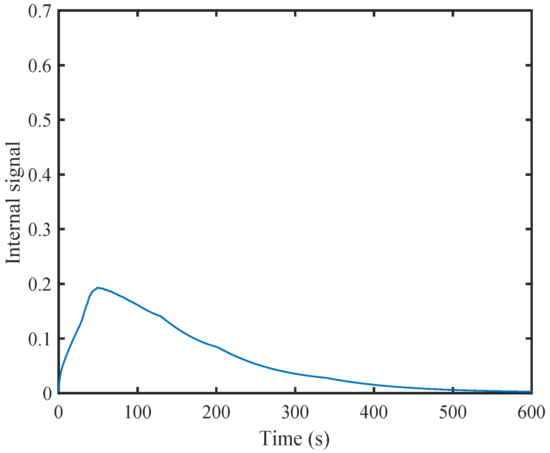
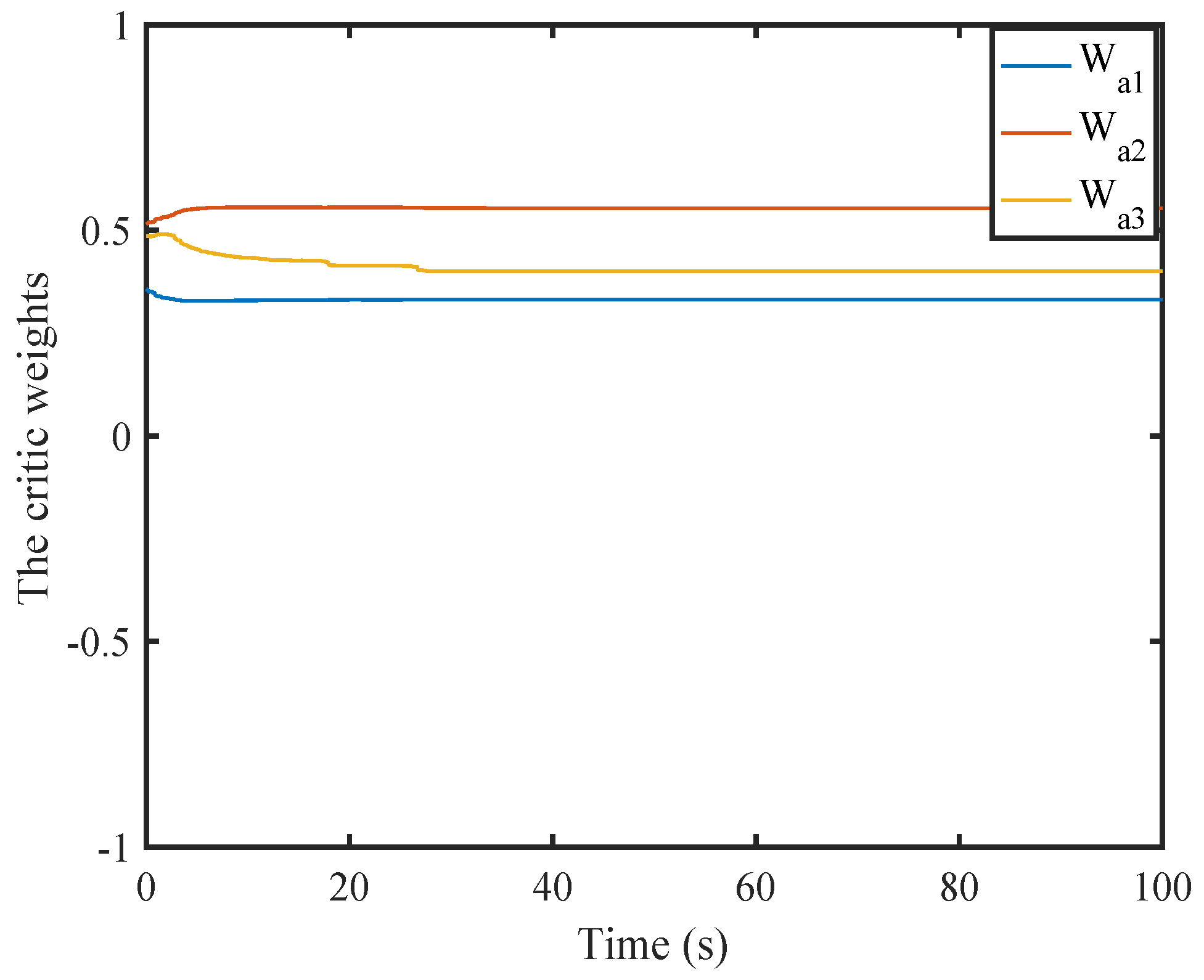
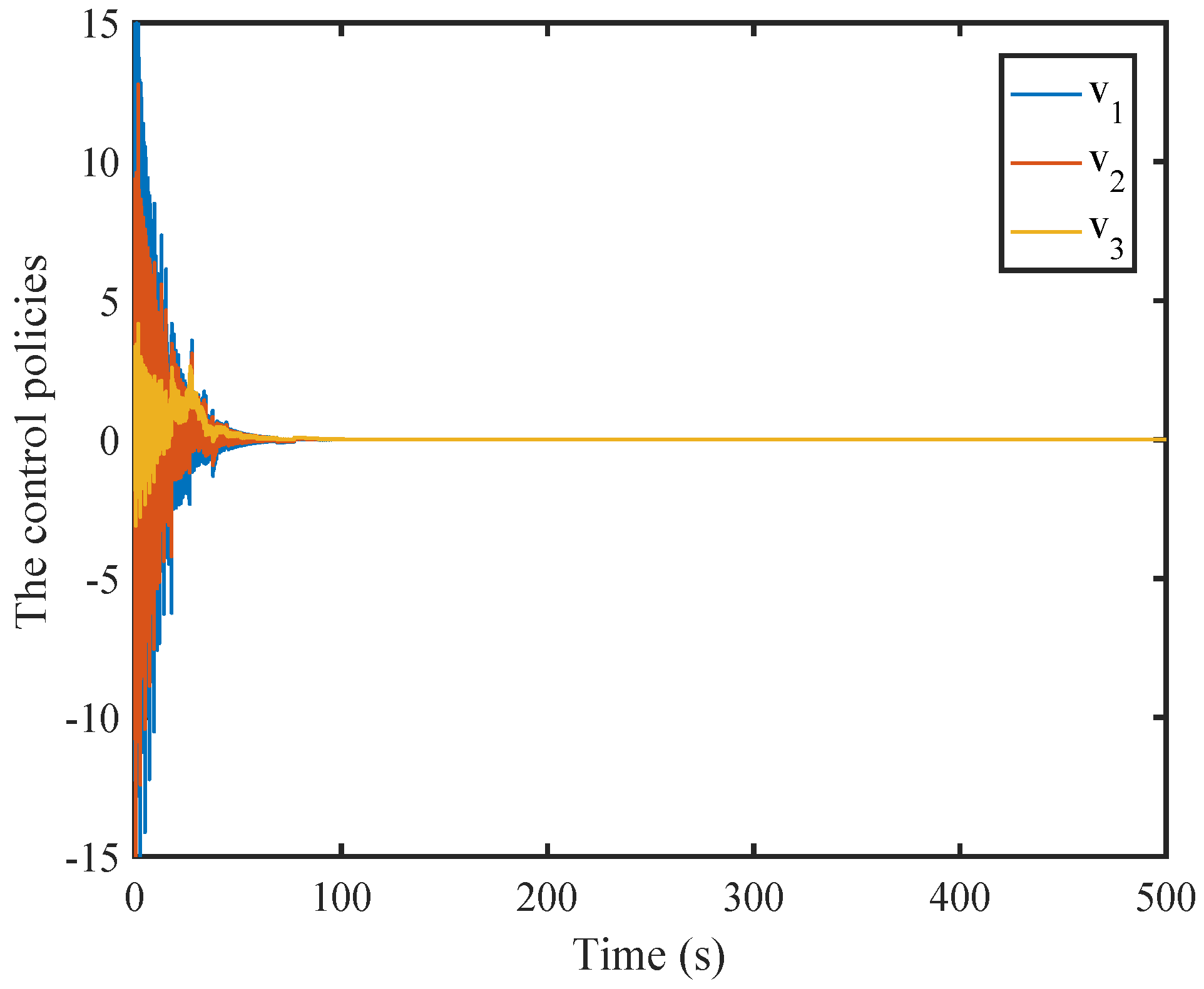
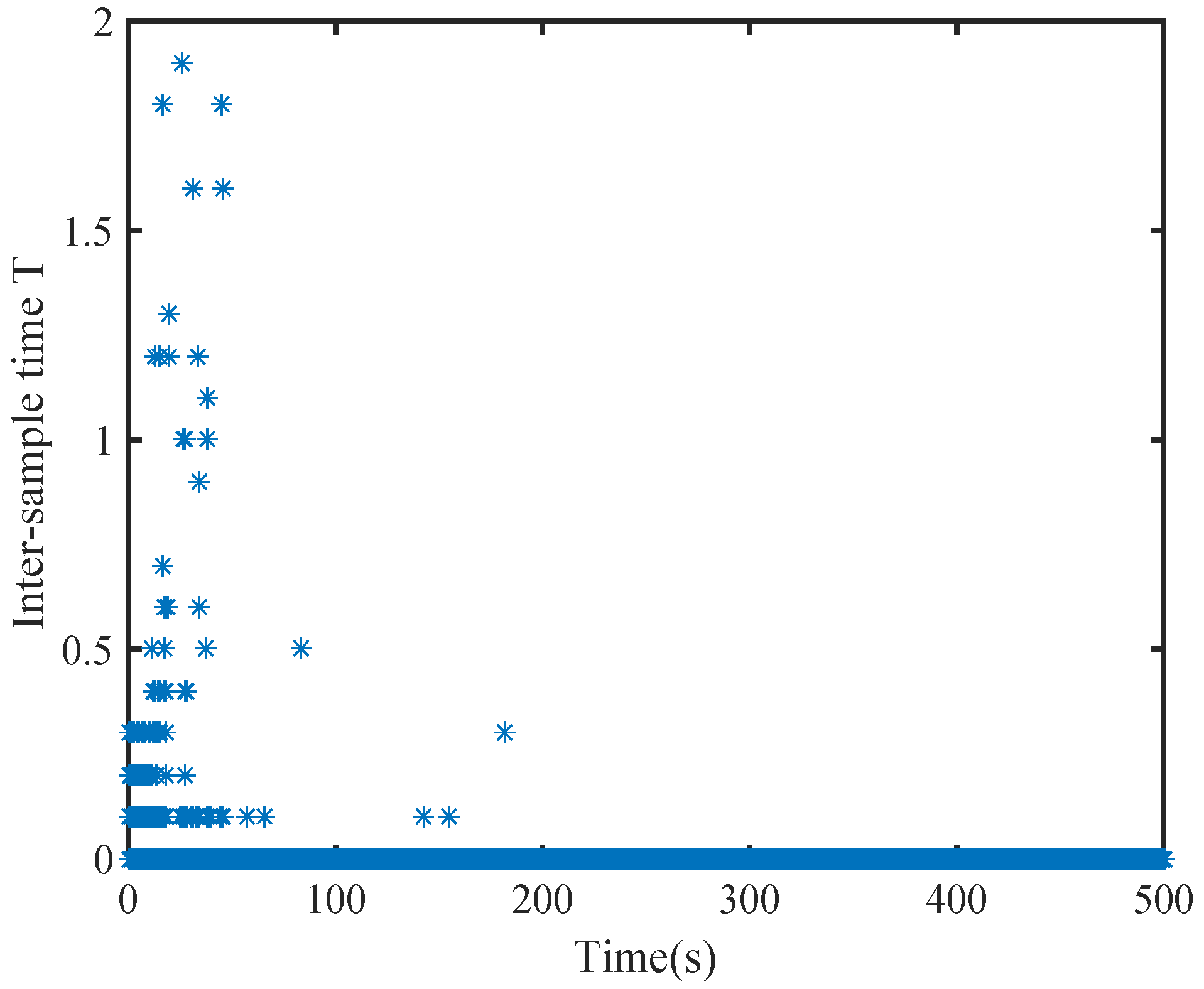
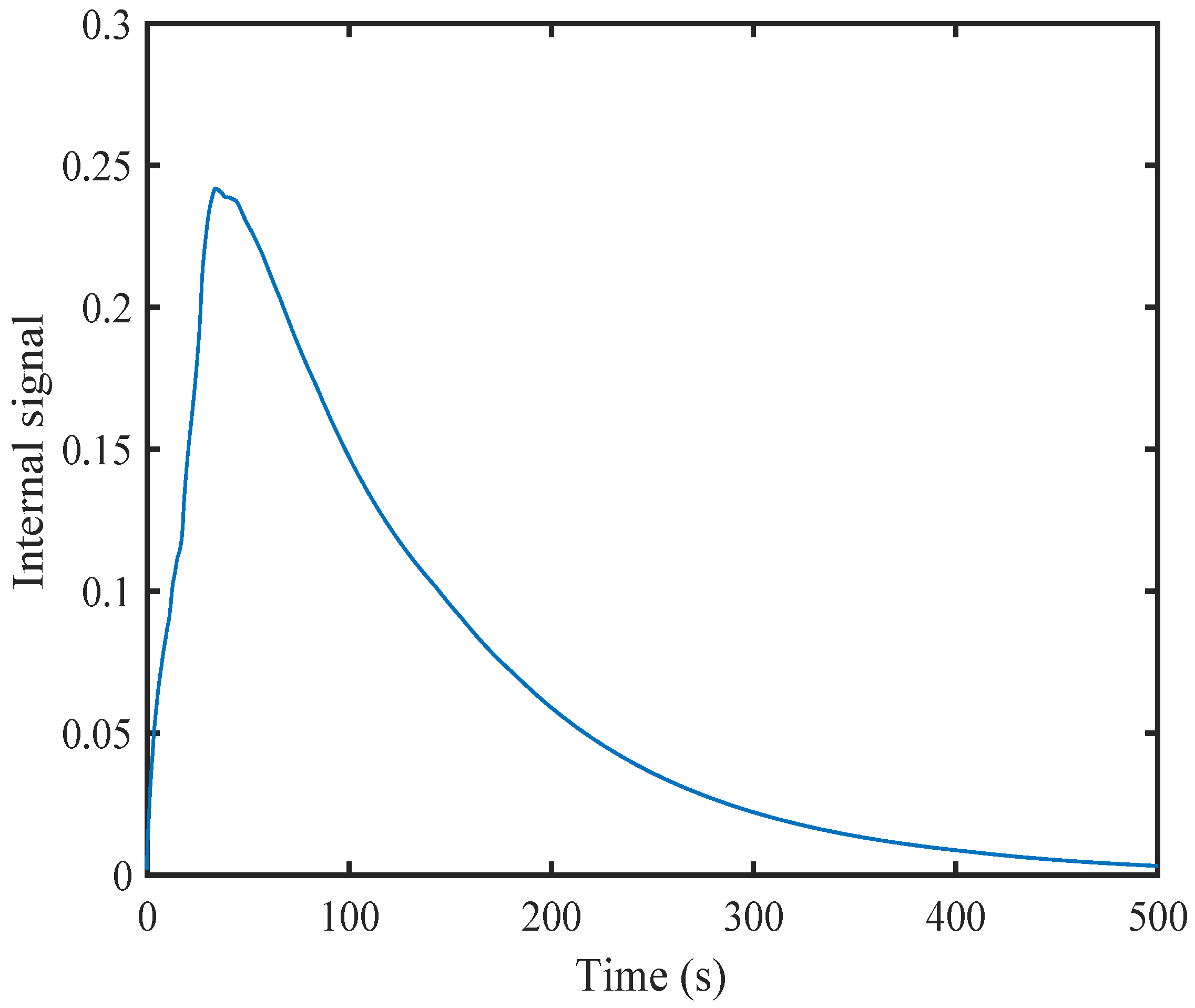
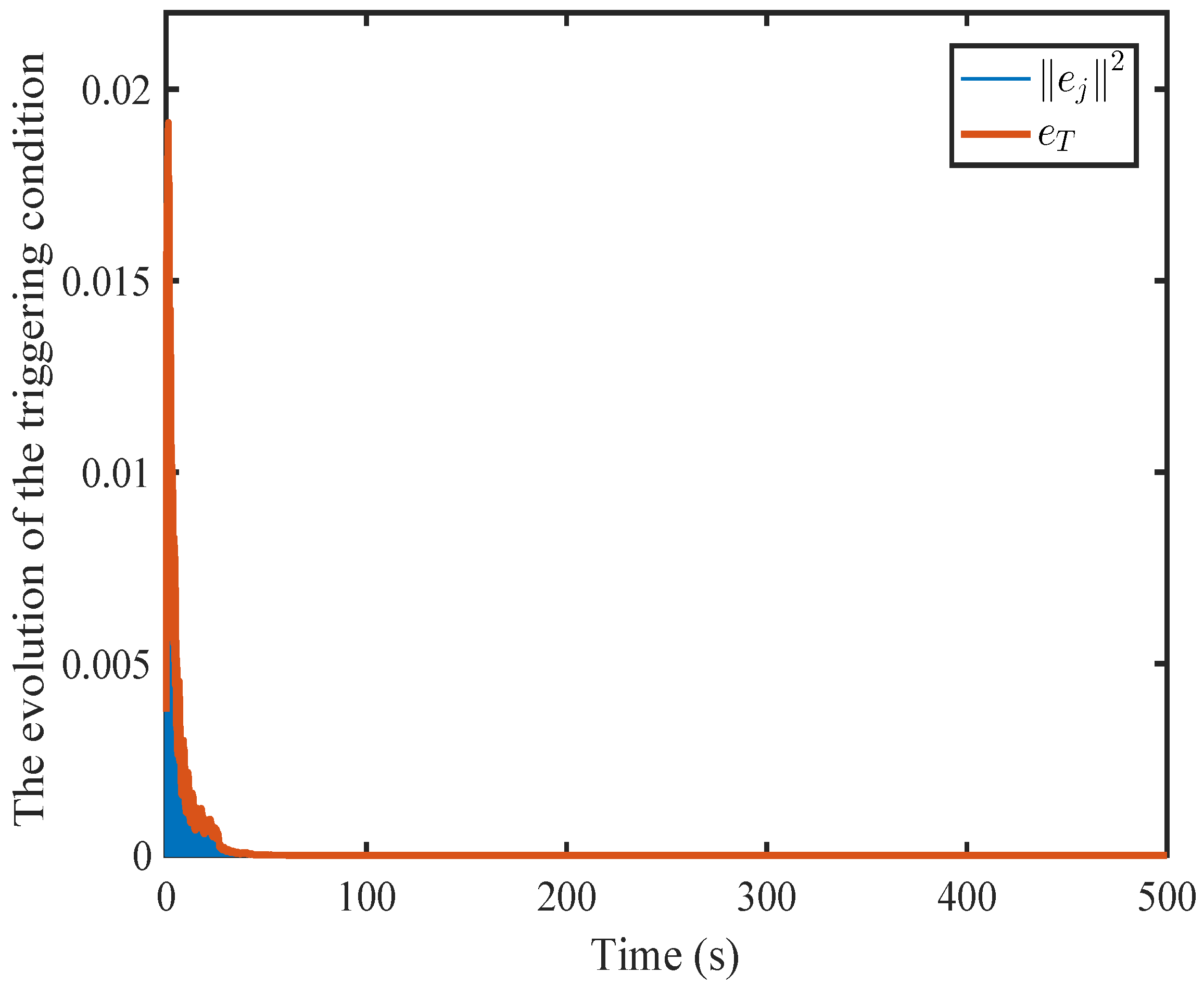
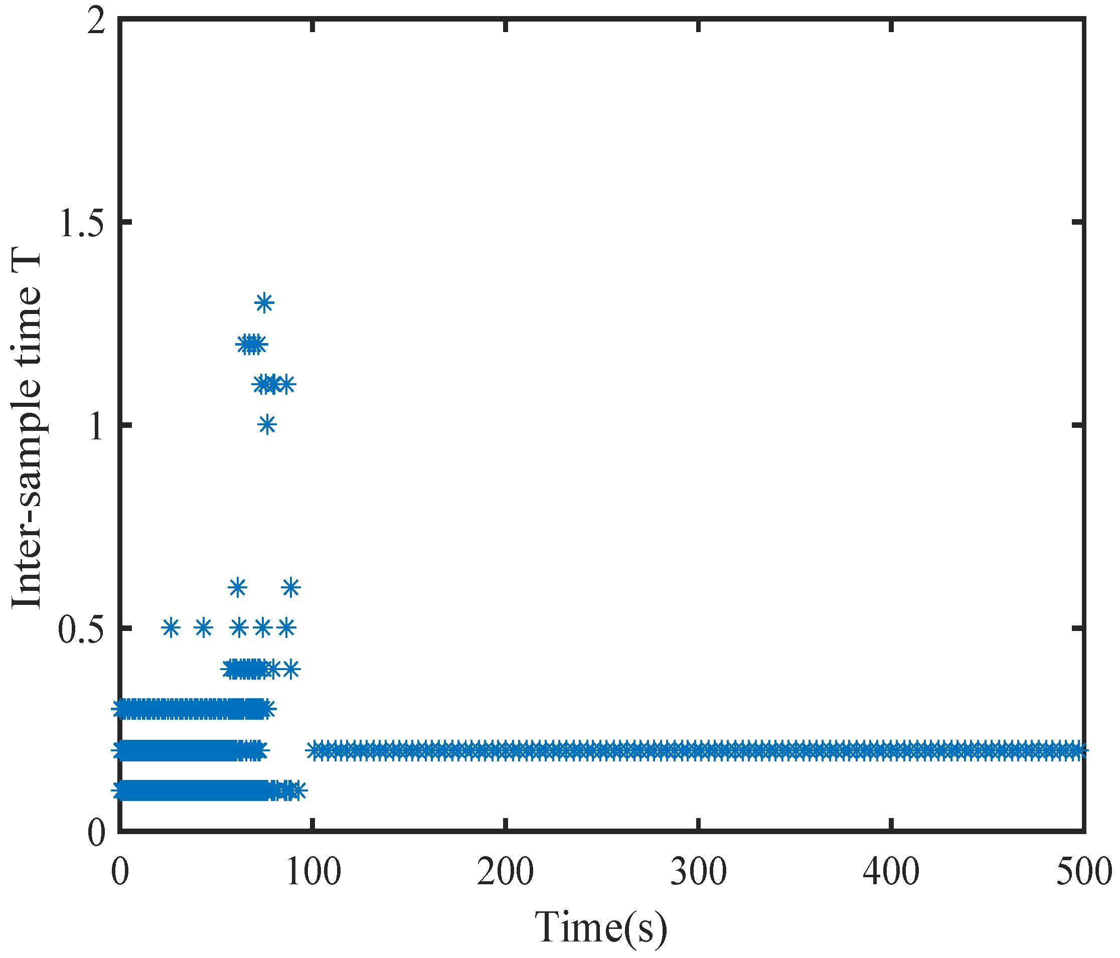
Theorem 3.

Assume that Assumptions 1–4 hold and the solution of Bellman Equation (31) exists. The DETC strategies are given in (39) and (41) for systems (1), and the augmented weight vector ${\widehat{\Gamma }}_i$ is updated based on (50). Providing the triggering condition is as

$$\begin{array}{c}\hfill {∥e_{k,i}∥}^2⩽{\displaystyle \frac{4({\sum }_{i=1}^N{\beta }_{1i}{\Re }_i-G\left({\overline{\vartheta }}_k\right)-{\sum }_{i=1}^N\mathbb{Z}\left({\overline{\vartheta }}_k\right))+{\varpi }^2{\lambda }_{min}\left(B\right){∥\vartheta ∥}^2}{4(L_u^2{\sum }_{i=1}^N{\sum }_{j=1}^N{∥{\overline{\mathfrak{r}}}_{i,j}∥}^2-2{\gamma }^{2}N{L}_u^2)}},\end{array}$$

(54)

where $G\left({\overline{\vartheta }}_k\right)$ and ${\mathbb{Z}}_i\left({\overline{\vartheta }}_k\right)$ are proposed in (59) and (64), $\varpi \in (0,1)$ is a design parameter.

$$\begin{array}{cc}\hfill {\dot{\Re }}_i=& -{\beta }_{1i}{\Re }_i+{\displaystyle \frac{{\varpi }^2{\lambda }_{min}\left(B\right){\parallel \vartheta \parallel }^2}{4N}}.\hfill \end{array}$$

(55)

Proof. 

The Lyapunov function is chosen as

$$\begin{array}{c}\hfill \Lambda ={\Lambda }_1+{\Lambda }_2+{\Lambda }_3,\end{array}$$

(56)

where ${\Lambda }_1={\mathbb{K}}_1+{\mathbb{K}}_2={\sum }_{i=1}^N{Q}_i^{*}\left(\vartheta \right)+{\sum }_{i=1}^N{\Re }_i$ with ${\mathbb{K}}_1={\sum }_{i=1}^N{Q}_i^{*}\left(\vartheta \right)$ and ${\mathbb{K}}_2={\sum }_{i=1}^N{\Re }_i$, ${\Lambda }_2={\sum }_{i=1}^N{\displaystyle \frac{1}{2{\lambda }_i}}{\tilde{\Gamma }}_i^T{\tilde{\Gamma }}_i$ and ${\Lambda }_3={\sum }_{i=1}^N{Q}_i^{*}\left({\overline{\vartheta }}_k\right)$.

Case 1: When $\forall t\in \left[t_k,t_{k+1}\right)$, $k\in \Gamma$, considering system dynamics (1) and applying the DETC policies in (45), it has ${\dot{\Lambda }}_1\left(t\right)={\dot{\mathbb{K}}}_1+{\dot{\mathbb{K}}}_2$ with ${\dot{\mathbb{K}}}_1={\sum }_{i=1}^N{\left(\nabla Q_i^{*}\left(\vartheta \right)\right)}^T(f\left(\vartheta \right)+{\sum }_{i=1}^{N+1}{h}_j{\widehat{v}}_{i,j}\left({\overline{\vartheta }}_k\right))$ and ${\dot{\mathbb{K}}}_2={\sum }_{i=1}^N{\dot{\Re }}_i$, ${\dot{\Lambda }}_2\left(t\right)={\sum }_{i=1}^N{\displaystyle \frac{1}{{\lambda }_i}}{\tilde{\Gamma }}_i^T{\dot{\tilde{\Gamma }}}_i$ and ${\dot{\Lambda }}_3\left(t\right)=0$.

Considering (38), ${\dot{\mathbb{K}}}_1\left(t\right)$ becomes

$$\begin{array}{c}\hfill \sum _{i=1}^N{\dot{Q}}_i\left(\vartheta \right)=\sum _{i=1}^N{W}_i^T\nabla {\varphi }_i\left(\vartheta \right)\left(f\left(\vartheta \right)+\sum _{j=1}^{N+1}{h}_j{\widehat{M}}_{i,j}^T{\phi }_{i,j}\left({\overline{\vartheta }}_k\right)\right)+\Im \left(x\right),\end{array}$$

(57)

where $\Im \left(\vartheta \right)={\sum }_{i=1}^N\nabla {\epsilon }_i\left(\vartheta \right)\left(f\left(\vartheta \right)+{\sum }_{j=1}^{k+1}{h}_j{\widehat{M}}_{i,j}^T{\phi }_{i,j}\left({\overline{\vartheta }}_k\right)\right)$.

Based on Equations (10)–(13), we have

$$\begin{array}{cc}\hfill \sum _{i=1}^N{\left(\nabla Q_i^{*}\left(\vartheta \right)\right)}^{T}f\left(\vartheta \right)=& -\sum _{i=1}^N{\vartheta }^T{B}_i\vartheta -\sum _{i=1}^N{\left(\nabla Q_i^{*}\left(\vartheta \right)\right)}^T{h}_{N+1}{v}_{i,N+1}^{*}\hfill \\ \hfill & +\sum _{i=1}^N\sum _{j=1}^N{v}_{i,j}^{*T}{R}_{i,j}{v}_{i,j}^{*}+{\gamma }^2{v}_{N,N+1}^{*T}{v}_{N,N+1}^{*}.\hfill \end{array}$$

(58)

In light of (10), (11), and (58) and based on the fact $R_{i,j}={\overline{\mathfrak{r}}}_{i,j}^T{\overline{\mathfrak{r}}}_{i,j}$ and Assumption 2, ${\dot{\mathbb{K}}}_1$ becomes

$$\begin{array}{cc}\hfill {\dot{\mathbb{K}}}_1& =-\sum _{i=1}^N{\vartheta }^T{B}_i\vartheta -2{\gamma }^2\sum _{i=1}^N{v}_{i,N+1}^{*T}\left(\vartheta \right)v_{i,N+1}^{*}\left(\vartheta \right)\hfill \\ \hfill & +\sum _{i=1}^N\sum _{j=1}^N{v}_{i,j}^{*T}\left(\vartheta \right)R_{i,j}{v}_{i,j}^{*}\left(\vartheta \right)+{\gamma }^2{v}_{N,N+1}^{*T}\left(\vartheta \right)v_{N,N+1}^{*}\left(\vartheta \right)\hfill \\ \hfill & -2\sum _{i=1}^N\sum _{j=1}^N{v}_{i,j}^{*T}\left(\vartheta \right)R_{i,j}{\widehat{v}}_{i,j}\left({\overline{\vartheta }}_k\right)+2{\gamma }^2\sum _{i=1}^N{v}_{i,N+1}^{*T}\left(\vartheta \right){\widehat{v}}_{i,N+1}\left({\overline{\vartheta }}_k\right)\hfill \\ \hfill & \le -{\vartheta }^{T}B\vartheta +\sum _{i=1}^N\sum _{j=1}^N{∥{\overline{\mathfrak{r}}}_{i,j}∥}^2{∥{\widehat{v}}_{i,j}\left({\overline{\vartheta }}_k\right)-v_{i,j}^{*}\left(\vartheta \right)∥}^2\hfill \\ \hfill & -\sum _{i=1}^N\sum _{j=1}^N{∥{\overline{\mathfrak{r}}}_{i,j}∥}^2{∥{\widehat{v}}_{i,j}\left({\overline{\vartheta }}_k\right)∥}^2-2{\gamma }^2\sum _{i=1}^N{∥{\widehat{v}}_{i,N+1}\left({\overline{\vartheta }}_k\right)-v_{i,N+1}^{*}\left(\vartheta \right)∥}^2\hfill \end{array}$$

$$\begin{array}{cc}\hfill & +2{\gamma }^2\sum _{i=1}^N{∥{\widehat{v}}_{i,N+1}\left({\overline{\vartheta }}_k\right)∥}^2+\mathcal{T}\hfill \\ \hfill & \le -{\vartheta }^{T}B\vartheta +(L_u^2\sum _{i=1}^N\sum _{j=1}^N{∥{\overline{\mathfrak{r}}}_{i,j}∥}^2-2{\gamma }^{2}N{L}_u^2){∥e_{k,i}∥}^2+\mathcal{T}\hfill \\ \hfill & -\sum _{i=1}^N\sum _{j=1}^N{∥{\overline{\mathfrak{r}}}_{i,j}∥}^2{∥{\widehat{v}}_{i,j}\left({\overline{\vartheta }}_k\right)∥}^2+2{\gamma }^2\sum _{i=1}^N{∥{\widehat{v}}_{i,N+1}\left({\overline{\vartheta }}_k\right)∥}^2\hfill \\ \hfill & =-{\vartheta }^{T}B\vartheta +(L_u^2\sum _{i=1}^N\sum _{j=1}^N{∥{\overline{\mathfrak{r}}}_{i,j}∥}^2-2{\gamma }^{2}N{L}_u^2){∥e_{k,i}∥}^2+G\left({\overline{\vartheta }}_k\right)\hfill \\ \hfill & \le -(1-{\displaystyle \frac{{\varpi }^2}{2}}){\vartheta }^{T}B\vartheta -{\displaystyle \frac{{\varpi }^2}{2}}{\lambda }_{min}\left(B\right){∥\vartheta ∥}^2\hfill \\ \hfill & +(L_u^2\sum _{i=1}^N\sum _{j=1}^N{∥{\overline{\mathfrak{r}}}_{i,j}∥}^2-2{\gamma }^{2}N{L}_u^2){∥e_{k,i}∥}^2+G\left({\overline{\vartheta }}_k\right),\hfill \end{array}$$

(59)

where B is given in (23) and $G\left({\overline{\vartheta }}_k\right)=\mathcal{T}-{\sum }_{i=1}^N{\sum }_{j=1}^N{∥{\overline{\mathfrak{r}}}_{i,j}∥}^2{∥{\widehat{v}}_{i,j}\left({\overline{\vartheta }}_k\right)∥}^2+2{\gamma }^2{\sum }_{i=1}^N{∥{\widehat{v}}_{i,N+1}\left({\overline{\vartheta }}_k\right)∥}^2$ where according to assumption 3, $\mathcal{T}$ is a normal number. And based on (49), we obtain

$$\begin{array}{c}\hfill {\overline{e}}_i=\overline{F}({\Gamma }_i-{\tilde{\Gamma }}_i)+{\int }_t^{t+T}\left({\vartheta }^T{B}_i\vartheta +{\widehat{U}}_i\right)ds,\end{array}$$

(60)

where ${\widehat{U}}_i={\sum }_{j=1}^N{\widehat{v}}_{i,j}^T\left({\overline{\vartheta }}_k\right)R_{i,j}{\widehat{v}}_{i,j}\left({\overline{\vartheta }}_k\right),i\in {\rm Y},i\ne N$ and ${\widehat{U}}_N={\sum }_{j=1}^N{\widehat{v}}_{N,j}^T\left({\overline{\vartheta }}_k\right)R_{N,j}{\widehat{v}}_{N,j}\left({\overline{\vartheta }}_k\right)-{\gamma }^2{\widehat{v}}_{N,N+1}^T\left({\overline{\vartheta }}_k\right){\widehat{v}}_{N,N+1}\left({\overline{\vartheta }}_k\right)$.

Based on (43) and (44), we have

$$\begin{array}{cc}\hfill & {\int }_t^{t+T}\left({\vartheta }^T{B}_i\vartheta +{\widehat{U}}_i\right)ds\hfill \\ \hfill =& {\int }_t^{t+T}(-W_i^T\nabla {\varphi }_i\left(\vartheta \right)f\left(\vartheta \right)-{\epsilon }_{HJI1}+{\widehat{U}}_i-{\overline{U}}_1+{\overline{U}}_2)dsi\in {\rm Y},i\ne N,\hfill \\ \hfill & {\int }_t^{t+T}\left({\vartheta }^T{B}_N\vartheta +{\widehat{U}}_N\right)ds\hfill \\ \hfill =& {\int }_t^{t+T}\left(-W_N^T\nabla {\varphi }_N\left(\vartheta \right)f\left(\vartheta \right)-{\epsilon }_{HJI2}+{\widehat{U}}_N-{\overline{U}}_3+{\overline{U}}_4\right.\hfill \end{array}$$

(61)

$$\begin{array}{c}\hfill \left.+{\gamma }^2{\left(M_{N,N+1}^T{\phi }_{N,N+1}\left({\overline{\vartheta }}_k\right)\right)}^T\left(M_{N,N+1}^T{\phi }_{N,N+1}\left({\overline{\vartheta }}_k\right)\right)\right)ds,\end{array}$$

(62)

where ${\overline{U}}_1={\sum }_{j=1}^N{\left(M_{i,j}^T{\phi }_{i,j}\left({\overline{\vartheta }}_k\right)\right)}^T{R}_{i,j}{M}_{i,j}^T{\phi }_{i,j}\left({\overline{\vartheta }}_k\right),{\overline{U}}_2=2{\sum }_{j=1}^{N+1}{\left(M_{i,j}^T{\phi }_{i,j}\left({\overline{\vartheta }}_k\right)\right)}^T{R}_{i,j}{M}_{i,j}^T{\phi }_{i,j}\left({\overline{\vartheta }}_k\right),{\epsilon }_{HJI1}⩽{\epsilon }_{hm1}$ and ${\overline{U}}_3={\sum }_{j=1}^N{\left(M_{N,j}^T{\phi }_{N,j}\left({\overline{\vartheta }}_k\right)\right)}^T{R}_{N,j}{M}_{N,j}^T{\phi }_{N,j}\left({\overline{\vartheta }}_k\right),{\overline{U}}_4=2{\sum }_{j=1}^{N+1}{\left(M_{N,j}^T{\phi }_{N,j}\left({\overline{\vartheta }}_k\right)\right)}^T{R}_{N,j}{M}_{N,j}^T{\phi }_{N,j}\left({\overline{\vartheta }}_k\right),{\epsilon }_{HJI2}\le {\epsilon }_{hm2}$. Define $S_{1i}={\int }_t^{t+T}\left({\overline{U}}_2-{\overline{U}}_1-{\epsilon }_{HJI1}\right)ds,S_{2i}={\int }_t^{t+T}\left({\widehat{U}}_i\right)ds,i\in {\rm Y},i\ne N,S_{3i}={\int }_t^{t+T}\left(-.W_i^T\nabla {\varphi }_i\left(\vartheta \right)f\left(\vartheta \right)\right)ds$ and $S_{1N}={\int }_t^{t+T}\left({\overline{U}}_4-{\overline{U}}_3-{\epsilon }_{HJI2}+\right.{\gamma }^2{\left(M_{N,N+1}^T{\phi }_{N,N+1}\left({\overline{\vartheta }}_k\right)\right)}^T{M}_{N,N+1}^T{\phi }_{N,N+1}\left({\overline{\vartheta }}_k\right)-{\gamma }^2{\left({\widehat{M}}_{N,N+1}^T{\phi }_{N,N+1}\left({\overline{\vartheta }}_k\right)\right)}^T{\widehat{M}}_{N,N+1}^T{\phi }_{N,N+1}\left.\left({\overline{\vartheta }}_k\right)\right)ds,S_{2N}={\int }_t^{t+T}\left({\sum }_{j=1}^N{\left({\widehat{M}}_{N,j}^T{\phi }_{N,j}\left({\overline{\vartheta }}_k\right)\right)}^T{R}_{N,j}{\widehat{M}}_{N,j}^T{\phi }_{N,j}\left({\overline{\vartheta }}_k\right)\right)ds$.

If the sampling interval T is sufficiently small, the integral terms $S_{1i}$, $S_{2i}$, $S_{3i}$, $S_{1N}$, and $S_{2N}$ can be approximated asb$S_{1i}=T\left({\overline{U}}_2-{\overline{U}}_1-{\epsilon }_{HJI1}\right),S_{2i}=T{\widehat{U}}_i,i\in {\rm Y},i\ne N,S_{3i}=T\left(-W_i^T\nabla {\varphi }_i\left(\vartheta \right)f\left(\vartheta \right)\right)$. When $i=N$, $S_{1N}=T\left({\overline{U}}_4-{\overline{U}}_3-{\epsilon }_{HJI2}+{\gamma }^2{\left(M_{N,j}^T{\phi }_{N,j}\left({\overline{\vartheta }}_k\right)\right)}^T{M}_{N,j}^T\right.\left.{\phi }_{N,j}\left({\overline{\vartheta }}_k\right)-{\gamma }^2{\left({\widehat{M}}_{N,j}^T{\phi }_{N,j}\left({\overline{\vartheta }}_k\right)\right)}^T{\widehat{M}}_{N,j}^T{\phi }_{N,j}\left({\overline{\vartheta }}_k\right)\right),S_{2N}=T{\sum }_{j=1}^N{\left({\widehat{M}}_{N,j}^T{\phi }_{N,j}\left({\overline{\vartheta }}_k\right)\right)}^T{R}_{N,j}{\widehat{M}}_{N,j}^T{\phi }_{N,j}\left({\overline{\vartheta }}_k\right)$.

Review Assumption 3; there is a constant $d_i$ that satisfies $∥S_{1i}∥\le d_i$.

Then, ${\mathcal{F}}_1=S_{1i}+S_{2i}+S_{3i}$. Thus, we have

$$\begin{array}{c}\hfill {\overline{e}}_i=\overline{\mathcal{F}}({\Gamma }_i-{\tilde{\Gamma }}_i)+S_{1i}+S_{2i}+S_{3i},i\in {\rm Y}.\end{array}$$

(63)

According to (50) and (60), one has

$$\begin{array}{cc}\hfill {\dot{\Lambda }}_2& =\sum _{i=1}^N{\displaystyle \frac{1}{{\lambda }_i}}{\tilde{\Gamma }}_i^T{\dot{\tilde{\Gamma }}}_i\hfill \\ \hfill & =\sum _{i=1}^N{\displaystyle \frac{{\tilde{\Gamma }}_i^T{\overline{\mathcal{F}}}^T}{{(\overline{\mathcal{F}}{\overline{\mathcal{F}}}^T+1)}^2}}\left(-\overline{\mathcal{F}}{\tilde{\Gamma }}_i+\overline{\mathcal{F}}{\Gamma }_i+S_{1i}+S_{2i}+S_{3i}\right)\hfill \\ \hfill & \le \sum _{i=1}^N(-{\tilde{\Gamma }}_i^T\overline{\rho }{\overline{\rho }}^T{\tilde{\Gamma }}_i+{\tilde{\Gamma }}_i^T\overline{\rho }{\overline{\rho }}^T{\Gamma }_i+{\displaystyle \frac{1}{2}}{d}_i∥{\tilde{\Gamma }}_i∥\hfill \\ \hfill & +{\displaystyle \frac{1}{4}}{∥{\tilde{\Gamma }}_i∥}^2+{\mathbb{Z}}_i\left({\overline{\vartheta }}_k\right)+{\displaystyle \frac{1}{4}}{∥{\tilde{\Gamma }}_i∥}^2+{\displaystyle \frac{1}{4}}{D}_1^2{∥\vartheta ∥}^2)\hfill \\ \hfill & \le \sum _{i=1}^N(-({\displaystyle \frac{m_1}{T}}-{\displaystyle \frac{1}{2}}){∥{\tilde{\Gamma }}_i∥}^2+{\mathbb{Z}}_i\left({\overline{\vartheta }}_k\right)+{\displaystyle \frac{1}{4}}{D}_1^2{∥\vartheta ∥}^2\hfill \\ \hfill & +\left({\displaystyle \frac{m_2}{T}}\sqrt{W_{i,\alpha }^2+M_{i,\alpha }^{\prime 2}}+{\displaystyle \frac{d_i}{2}}\right)∥{\tilde{\Gamma }}_i∥),i\in {\rm Y},\hfill \end{array}$$

(64)

where $\mathbb{Z}\left({\overline{\vartheta }}_k\right)={\displaystyle \frac{T^2}{4}}{\left({\sum }_{j=1}^N{\widehat{v}}_{i,j}^T\left({\overline{\vartheta }}_k\right)R_{i,j}{\widehat{v}}_{i,j}\left({\overline{\vartheta }}_k\right)\right)}^2$ and $D_1=T{W}_{i,\alpha }{\varphi }_{i,\beta }{\mathbb{B}}_f$.

Using (55), (56), (59), and (64), $\dot{\Lambda }$ becomes

$$\begin{array}{cc}\hfill \dot{\Lambda }\le & \left(-\sum _{i=1}^N{\beta }_{1i}{\mathfrak{R}}_i-(1-{\displaystyle \frac{{\varpi }^2}{2}}){\vartheta }^{T}B\vartheta -{\displaystyle \frac{{\varpi }^2}{4}}{\lambda }_{min}\left(B\right){∥\vartheta ∥}^2\right.\hfill \\ & \left.+(L_u^2\sum _{i=1}^N\sum _{j=1}^N{∥{\overline{\mathfrak{r}}}_{i,j}∥}^2-2{\gamma }^{2}N{L}_u^2){∥e_{k,i}∥}^2+G\left({\overline{\vartheta }}_k\right)\right)\hfill \\ \hfill & +\sum _{i=1}^N\left(-({\displaystyle \frac{m_1}{T}}-{\displaystyle \frac{1}{2}}){∥{\tilde{\Gamma }}_i∥}^2+{\mathbb{Z}}_i\left({\overline{\vartheta }}_k\right)+{\displaystyle \frac{1}{4}}{D}_1^2{∥\vartheta ∥}^2\right.\hfill \end{array}$$

$$\begin{array}{c}\hfill \left.+\left({\displaystyle \frac{m_2}{T}}\sqrt{W_{i,\alpha }^2+M_{i,\alpha }^{\prime 2}}+{\displaystyle \frac{d_i}{2}}\right)∥{\tilde{\Gamma }}_i∥\right).\end{array}$$

(65)

If the triggering condition (54) is satisfied, we have

$$\begin{array}{cc}\dot{\Lambda }\hfill & \le -(1-{\displaystyle \frac{{\varpi }^2}{2}}){\vartheta }^{T}B\vartheta -\sum _{i=1}^N\left(({\displaystyle \frac{m_1}{T}}-{\displaystyle \frac{1}{2}}){∥{\tilde{\Gamma }}_i∥}^2+{\displaystyle \frac{1}{4}}{D}_1^2{∥\vartheta ∥}^2\right.\hfill \\ & \left.+\left({\displaystyle \frac{m_2}{T}}\sqrt{W_{i,\alpha }^2+M_{i,\alpha }^{\prime 2}}+{\displaystyle \frac{d_i}{2}}\right)∥{\tilde{\Gamma }}_i∥\right)\hfill \\ \hfill & \le -(1-{\displaystyle \frac{{\varpi }^2}{2}}){\vartheta }^{T}B\vartheta -\sum _{i=1}^N{ð}_1{\left(\parallel {\tilde{\Gamma }}_i\parallel -{\displaystyle \frac{2m_2\sqrt{W_{i,\alpha }^2+M_{i,\alpha }^{\prime 2}}+T{d}_i}{2\left(2m_1-T\right)}}\right)}^2\hfill \\ \hfill & +\sum _{i=1}^N(m_3+{ð}_2{\parallel \vartheta \parallel }^2),\hfill \end{array}$$

(66)

where ${ð}_1=\left({\displaystyle \frac{m_1}{T}}-{\displaystyle \frac{1}{2}}\right),{ð}_2={\displaystyle \frac{1}{4}}{D}_1^2,m_3={\displaystyle \frac{{\left(2m_2\sqrt{W_{i,\alpha }^2+M_{i,\alpha }^{\prime 2}}+d_{i}T\right)}^2}{8T\left(2m_1-T\right)}}$.

Let the parameter $\varpi$, $m_1$ and the interval T be chosen such that ${\varpi }^2{\lambda }_{min}\left(B\right)-1/4D_1^2>0$ and $m_1>{\displaystyle \frac{T}{2}}$. Then, $\dot{\Lambda }\left(t\right)<0$ if

$$\begin{array}{cc}\hfill ∥\vartheta ∥& >\sqrt{{\displaystyle \frac{m_3}{{ð}_2}}},\hfill \\ \hfill ∥{\tilde{\Gamma }}_i∥& >\sqrt{{\displaystyle \frac{m_3}{{ð}_1}}}+{\displaystyle \frac{2m_2\sqrt{W_{i,\alpha }^2+M_{i,\alpha }^{\prime 2}}+T{d}_i}{2\left(2m_1-T\right)}}.\hfill \end{array}$$

(67)

Therefore, the system states and the NN weight estimation errors are UUB.

Case 2: When $\forall t=t_{k+1}$, the differential of this function can be expressed as

$$\begin{array}{cc}\hfill \Delta \Lambda \left(t\right)=& {\displaystyle \frac{1}{2}}{\tilde{\Gamma }}_i^T\left(\overline{\vartheta }\left(t_k^{+}\right)\right){\tilde{\Gamma }}_i\left(\overline{\vartheta }\left(t_k^{+}\right)\right)\hfill \\ \hfill & -{\displaystyle \frac{1}{2}}{\tilde{\Gamma }}_i^T\left(\overline{\vartheta }\left(t_k\right)\right){\tilde{\Gamma }}_i\left(\overline{\vartheta }\left(t_k\right)\right)\hfill \\ \hfill & +Q_i^{*}\left({\overline{\vartheta }}_{k+1}\right)-Q_i^{*}\left({\overline{\vartheta }}_k\right)+Q_i^{*}\left(\overline{\vartheta }\left(t_k^{*}\right)\right)-Q_i^{+}\left({\overline{t}}_k\right).\hfill \end{array}$$

(68)

Based on Case 1, $Q\left(t\right)$ is monotonically decreasing on $[t_k,t_{k+1})$. Thus, one obtains $Q(t_k+\aleph )<Q\left(t_k\right)$, $\aleph \in (0,t_{k+1}-t_k)$. Applying the limit to each side of the inequality, it has $\Lambda \left(t_k^{+}\right)\le \Lambda \left(t_k\right)$. Based on that fact, we have

$$\begin{array}{c}{Q}_i^{*}\left(\overline{\vartheta }\left(s_k^{+}\right)\right)+{\displaystyle \frac{1}{2}}{\tilde{\Gamma }}_i^T\left(\overline{\vartheta }\left(t_k^{+}\right)\right){\tilde{\Gamma }}_i\left(\overline{\vartheta }\left(t_k^{+}\right)\right)\hfill \\ \le Q_i^{*}\left(\overline{\vartheta }\left(t_k\right)\right)+{\displaystyle \frac{1}{2}}{\tilde{\Gamma }}_i^T\left(\overline{\vartheta }\left(t_k\right)\right){\tilde{\Gamma }}_i\left(\overline{\vartheta }\left(t_k\right)\right).\hfill \end{array}$$

(69)

Moreover, $Q_i^{*}\left(\vartheta \right)$ is a continuous difference function at the triggering instant $t_k$ with $k\in \Gamma$. According to the results of Case 1, one has $Q_i^{*}\left({\overline{\vartheta }}_{k+1}\right)\le Q_i^{*}\left({\overline{\vartheta }}_k\right)$. According to the analysis presented above, it obtains $\Delta \Lambda \left(t\right)\le 0$. □

6. Simulation

In this section, examples of connecting two nonlinear systems are provided to verify the effectiveness of the algorithm.

6.1. A Nonlinear Example

In this example, to assess the efficacy of our method, we consider four players by [39]:

$$\begin{array}{cc}\hfill \dot{\vartheta }& =\left[\begin{array}{c}{\vartheta }_2\\ -0.5{\vartheta }_1-0.5{\vartheta }_2\left(1+{\left(cos\left(2{\vartheta }_1\right)+2\right)}^2\right)\end{array}\right]\hfill \\ \hfill & +\left[\begin{array}{c}0\\ sin\left({\vartheta }_1\right)\end{array}\right]v_1\left(\vartheta \right)+\left[\begin{array}{c}0\\ 2cos\left(2{\vartheta }_1\right)+4\end{array}\right]v_2\left(\vartheta \right)\hfill \\ \hfill & +\left[\begin{array}{c}0\\ sin\left({\vartheta }_2\right)\end{array}\right]v_3\left(\vartheta \right)+\left[\begin{array}{c}0\\ 2sin\left(2{\vartheta }_1\right)+4\end{array}\right]d_1\left(\vartheta \right).\hfill \end{array}$$

(70)

Define the cost performances as

$$\begin{array}{cc}\hfill Q_1& ={\int }_{t=0}^{\infty }{\vartheta }^T{B}_1\vartheta +v_1^T{R}_{11}{v}_1+v_2^T{R}_{12}{v}_2+v_3^T{R}_{13}{v}_{3}ds,\hfill \end{array}$$

(71)

$$\begin{array}{cc}\hfill Q_2& ={\int }_{t=0}^{\infty }{\vartheta }^T{B}_2\vartheta +v_1^T{R}_{21}{v}_1+v_2^T{R}_{22}{v}_2+v_3^T{R}_{23}{v}_{3}ds,\hfill \end{array}$$

(72)

$$\begin{array}{cc}\hfill Q_3& ={\int }_{t=0}^{\infty }{\vartheta }^T{B}_3\vartheta +v_1^T{R}_{31}{v}_1+v_2^T{R}_{32}{v}_2+v_3^T{R}_{33}{v}_3-{\gamma }^2{d}_1^T{d}_{1}ds.\hfill \end{array}$$

(73)

Set $\gamma =8$, $R_{11}=R_{12}=R_{13}=R_{21}=R_{22}=R_{23}=2I$, $R_{31}=R_{32}=R_{33}=I$, and I has appropriate dimensions, and let $B_1=B_2=\left[\begin{array}{cc}9& 0\\ 0& 9\end{array}\right]$, $B_3=\left[\begin{array}{cc}5& 0\\ 0& 5\end{array}\right]$. The values of other quantities are the same as the previous simulation.

In the design, assume that the all initial probing control inputs are $a=37e^{-0.061t}({sin}^2\left(t\right)cos\left(t\right)+{sin}^2\left(2t\right)cos\left(0.1t\right))$. The simulation parameters are shown in

Table 1. Parameter settings.

simulation 1	$\gamma$	${\lambda }_i$	${\beta }_1$	${\beta }_2$	$\sigma$	$L_u$	$\omega$
	8	0.75	0.1	0.1	0.1	1.2	0.5
simulation 2	$\gamma$	${\lambda }_i$	${\beta }_1$	${\beta }_2$	$\sigma$	$L_u$	$\omega$
	5	0.7	0.1	0.1	0.1	1.2	0.5

.

The weight values of the first critic NN converge to [0.0735, −0.0450, −0.0391, 0.0933, −0.0863, 0.0406, −0.0506, 0.0049].

The weight values of the second critic NN converge to [0.0630, 0.1011, −0.0737, 0.0608, −0.0660, 0.0269, −0.0443, −0.0504].

The weight values of the third critic NN converge to [−0.0478, 0.0633, −0.0894, 0.0563, −0.0596, 0.0573, −0.0492, −0.0533].

The weight values of the first actor NN converge to [−0.0841, 0.0986, −0.0840, −0.0064, 0.1016, −0.0182, −0.0609, −0.0122].

The weight values of the second actor NN converge to [0.0368, 0.0522, −0.0989, −0.0856, 0.0639, −0.0972, −0.0370, 0.0443].

The weight values of the third actor NNconverge to [−0.0234, 0.0595, −0.0533, 0.0918, −0.0593, −0.0925, 0.1057, 0.0467].

The weight values of the fourth actor NN converge to [−0.0901, −0.0371, −0.0823, −0.0966, 0.0726, 0.0672, −0.0004, 0.0482].

It is clear that the system state converges to zero.

It is obvious that the control input converges to zero.

It can be found that the norm of sampling error under dynamic event-triggering converges to zero.

It is obvious that compared to static event-triggering, the number of actuator updates triggered by dynamic events decreased by 55%.

It can be found that the internal dynamic signals converges to zero.

Figure 2, Figure 3, Figure 4, Figure 5, Figure 6, Figure 7, Figure 8, Figure 9, Figure 10, Figure 11, Figure 12, Figure 13, Figure 14 and Figure 15 display the simulation results. Figure 2, Figure 3, Figure 4, Figure 5, Figure 6, Figure 7 and Figure 8 show the convergence of the weight vectors of the critic and actor NNs.

It is clear that the norm of sampling error under static event-triggering converges to zero.

In Figure 12 and Figure 15, the horizontal axis of symbol “*” represents the triggering instant, and the vertical axis of symbol “*” denotes the difference between the current triggering instant and the previous triggering instant. The evolutions of the system states and the control inputs are displayed in Figure 9 and Figure 10, respectively. They illustrate that the system will rapidly converge to zero. The Figure 11 and Figure 14, respectively, provide curves of the sampling error norms triggered by dynamic and static events and the triggering threshold specifications. The sampling times triggered by dynamic and static events are shown in Figure 10 and Figure 15. Figure 13 shows the internal signal. From the graph, it can be seen that the internal signal is positive.

By comparison, it is evident that dynamic event-triggering strategies containing dynamic internal signals have larger thresholds and fewer event-triggering times. Compared to static event-triggering, the number of actuator updates have been reduced by 55%. This indicates that compared to other triggering mechanisms, the dynamic event-triggering mechanism proposed in this paper can significantly reduce computational complexity.

6.2. A Comparison Simulation

Consider the following system dynamics in [38]

$$\begin{array}{cc}\hfill \dot{\vartheta }& =\left[\begin{array}{c}\left({\vartheta }_2-2{\vartheta }_1\right)\\ (-{\displaystyle \frac{1}{2}}{\vartheta }_1-{\vartheta }_2+{\displaystyle \frac{1}{4}}{\vartheta }_2{\left(cos\left(2{\vartheta }_1+2\right)\right)}^2\\ +{\displaystyle \frac{1}{4}}{\vartheta }_2{\left(sin\left(4{\vartheta }_1^2\right)+2\right)}^2)\end{array}\right]+\left[\begin{array}{c}0\\ cos\left(2{\vartheta }_1\right)+2\end{array}\right]v_1\left(\vartheta \right)\hfill \\ \hfill & +\left[\begin{array}{c}0\\ sin\left(4{\vartheta }_1^2\right)+2\end{array}\right]v_2\left(\vartheta \right)+\left[\begin{array}{c}0\\ sin\left(4{\vartheta }_1\right)+2\end{array}\right]d_1\left(\vartheta \right).\hfill \end{array}$$

(74)

Define the cost performances as

$$\begin{array}{cc}\hfill Q_1& ={\int }_{t=0}^{\infty }{\vartheta }^T{B}_1\vartheta +v_1^T{R}_{11}{v}_1+v_2^T{R}_{12}{v}_{2}ds,\hfill \end{array}$$

(75)

$$\begin{array}{cc}\hfill Q_2& ={\int }_{t=0}^{\infty }{\vartheta }^T{B}_2\vartheta +v_1^T{R}_{21}{v}_1+v_2^T{R}_{22}{v}_2-{\gamma }^2{d}_1^T{d}_{1}ds.\hfill \end{array}$$

(76)

Set $\gamma =8$, $R_{11}=R_{12}=2I$, $R_{21}=R_{22}=I$, and I has appropriate dimensions, $B_1=\left[\begin{array}{cc}2& 0\\ 0& 2\end{array}\right]$, and $B_2=\left[\begin{array}{cc}1& 0\\ 0& 1\end{array}\right]$. For critic NNs, the initial weights are set to [−0.1, 0.1], and the initial weight vectors of the actor NNs are randomly set in the interval $[-1,1]$. Select the NN activation function as ${\varphi }_i\left(\vartheta \right)={\phi }_{i,j}\left(\vartheta \right)={[{\vartheta }_1^2,{\vartheta }_1{\vartheta }_2,{\vartheta }_2^2]}^T$. The initial system state is ${\vartheta }_0={[-1,1]}^T$, and set the sampling time as $T=0.005$ s. Moreover, select the parameter ${\lambda }_i=0.75$. The probing control inputs are added, which are $a=37e^{-0.061t}({sin}^2\left(t\right)cos\left(t\right)+{sin}^2\left(2t\right)cos\left(0.1t\right))$.

The weight values of the first critic NN converge to $\left[0.3315,0.5437,0.4726\right]$.

The weight values of the second critic NN converge to $\left[0.0832,0.5894,-0.1181\right]$.

The weight values of the first actor NN converge to $\left[-0.1354,0.1913,-0.4494\right]$.

The weight values of the second actor NN converge to $\left[0.4913,-1.054,-0.2434\right]$.

The weight values of the third actor NN converge to $\left[-0.8691,-0.8623,-0.5519\right]$.

It is clear that the system state converges to zero.

Figure 16, Figure 17, Figure 18, Figure 19 and Figure 20 illustrate the convergence of the critic and actor NNs weight vector. The evolutions of the system states and the control inputs are displayed in Figure 21 and Figure 22, which show that the system states converge and the control signals rapidly converge to zero. Figure 23 and Figure 24 present the norm of the sampling error ${∥e_j∥}^2$ and the norm of the trigger threshold $e_T$, and the sampling time $T_1$, respectively. The internal dynamic signals $\mathfrak{R}$ are depicted in Figure 25. It can be seen that the internal signal is positive.

It is obvious that the control input converges to zero.

It can be found that the norm of sampling error under dynamic event-triggering converges to zero.

To highlight the benefits of the proposed dynamic event-triggering mechanism, Figure 26 and Figure 27 show the sampling error, threshold norm, and the sample interval of the systems under the static event-triggering condition. By comparing Figure 23 and Figure 24 with Figure 26 and Figure 27, it is evident that the dynamic event-triggering strategy incorporating the positive dynamic internal signal $\mathfrak{R}$ has a larger threshold and fewer event-triggering occurrences. The dynamic event-triggering mechanism introduced in this paper can significantly reduce the computational burden.

In Figure 24 and Figure 27, the horizontal axis of symbol “*” represents the triggering instant, and the vertical axis of symbol “*” denotes the difference between the current triggering instant and the previous triggering instant.

It can be found that compared to static event-triggering, the number of actuator updates triggered by dynamic events decreased by 69%.

It can be found that the internal dynamic signals converges to zero.

It is clear that the norm of sampling error under static event-triggering converges to zero.

7. Conclusions

In this paper, a DETC approach based on IRL has been designed for the MZSG problem in nonlinear systems with completely unknown dynamics. This algorithm has relaxed the requirements on the system drift dynamics. In the adaptive control process, an actor–critic approach has been adopted to design synchronized adjustment rules for weight updates. The IRL algorithm designed in this framework has been implemented online, providing a new approach for combining NN and DETC to solve the MZSG problem. The method has proposed dynamic event-triggering conditions, which reduces communication resources for the controlled object. Finally, the effectiveness of the proposed method has been validated through two examples. The simulation results show that the number of actuator updates in the DETC mechanism has been reduced by 55% and 69%, respectively, compared with static event-triggering mode.

References

1. Chen, L.; Yu, Z.Y. Maximum principle for nonzero-sum stochastic differential game with delays. IEEE Trans. Automa. Control 2014, 60, 1422–1426. [Google Scholar] [CrossRef]
2. Yasini, S.; Sitani, M.B.N.; Kirampor, A. Reinforcement learning and neural networks for multi-agent nonzero-sum games of nonlinear constrained-input systems. Int. J. Mach. Learn. Cybern. 2016, 7, 967–980. [Google Scholar] [CrossRef]
3. Rupnik Poklukar, D.; Žerovnik, J. Double Roman Domination: A Survey. Mathematics 2023, 11, 351. [Google Scholar] [CrossRef]
4. Leon, J.F.; Li, Y.; Peyman, M.; Calvet, L.; Juan, A.A. A Discrete-Event Simheuristic for Solving a Realistic Storage Location Assignment Problem. Mathematics 2023, 11, 1577. [Google Scholar] [CrossRef]
5. Tanwani, A.; Zhu, Q.Y.Z. Feedback nash equilibrium for randomly switching differential-algebraic games. IEEE Trans. Automa. Control 2020, 65, 3286–3301. [Google Scholar] [CrossRef]
6. Peng, B.W.; Stancu, A.; Dang, S.P. Differential graphical games for constrained autonomous vehicles based on viability theory. IEEE Trans. Cybern. 2022, 52, 8897–8910. [Google Scholar] [CrossRef]
7. Wu, S. Linear-quadratic non-zero sum backward stochastic differential game with overlapping information. IEEE Trans. Autom. Control 2023, 60, 1800–1806. [Google Scholar] [CrossRef]
8. Dong, B.; Feng, Z.; Cui, Y.M. Event-triggered adaptive fuzzy optimal control of modular robot manipulators using zero-sum differential game through value iteration. Int. J. Adapt. Control Signal Process. 2023, 37, 2364–2379. [Google Scholar] [CrossRef]
9. Wang, D.; Zhao, M.M.; Ha, M.M. Stability and admissibility analysis for zero-sum games under general value iteration formulation. IEEE Trans. Neural Netw. Learn. Syst. 2023, 34, 8707–8718. [Google Scholar] [CrossRef]
10. Du, W.; Ding, S.F.; Zhang, C.L. Modified action decoder using Bayesian reasoning for multi-agent deep reinforcement learning. Int. J. Mach. Learn. Cybern. 2021, 12, 2947–2961. [Google Scholar] [CrossRef]
11. Lv, Y.F.; Ren, X.M. Approximate nash solutions for multiplayer mixed-zero-sum game with reinforcement learning. IEEE Trans. Syst. Man Cybern. Syst. 2019, 49, 2739–2750. [Google Scholar] [CrossRef]
12. Qin, C.B.; Zhang, Z.W.; Shang, Z.Y. Adaptive optimal safety tracking control for multiplayer mixed zero-sum games of continuous-time systems. Appl. Intell. 2023, 53, 17460–17475. [Google Scholar] [CrossRef]
13. Ming, Z.Y.; Zhang, H.G.; Zhang, J.; Xie, X.P. A novel actor-critic-identifier architecture for nonlinear multiagent systems with gradient descent method. Automatica 2023, 155, 645–657. [Google Scholar] [CrossRef]
14. Ming, Z.Y.; Zhang, H.G.; Wang, Y.C.; Dai, J. Policy iteration Q-learning for linear ito stochastic systems with markovian jumps and its application to power systems. IEEE Trans. Cybern. 2024, 54, 7804–7813. [Google Scholar] [CrossRef] [PubMed]
15. Song, R.Z.; Liu, L.; Xia, L.; Frank, L. Online optimal event-triggered H control for nonlinear systems with constrained state and input. IEEE Trans. Syst. Man Cybern. Syst. 2023, 53, 1–11. [Google Scholar] [CrossRef]
16. Liu, Y.; Zhang, H.G.; Yu, R. H tracking control of discrete-time system with delays via data-based adaptive dynamic programming. IEEE Trans. Syst. Man Cybern. Syst. 2020, 50, 4078–4085. [Google Scholar] [CrossRef]
17. Zhang, H.G.; Liu, Y.; Xiao, G.Y. Data-based adaptive dynamic programming for a class of discrete-time systems with multiple delays. IEEE Trans. Syst. Man Cybern. Syst. 2020, 50, 432–441. [Google Scholar] [CrossRef]
18. Wang, R.G.; Wang, Z.; Liu, S.X. Optimal spin polarization control for the spin-exchange relaxation-free system using adaptive dynamic programming. IEEE Trans. Neural Netw. Learn. Syst. 2024, 35, 5835–5847. [Google Scholar] [CrossRef]
19. Wen, Y.; Si, J.; Brandt, A. Online reinforcement learning control for the personalization of a robotic knee prosthesis. IEEE Trans. Cybern. 2020, 50, 2346–2356. [Google Scholar] [CrossRef]
20. Yu, S.H.; Zhang, H.G.; Ming, Z.Y. Adaptive optimal control via continuous-time Q-learning for Stackelberg-Nash games of uncertain nonlinear systems. IEEE Trans. Syst. Man Cybern. Syst. 2023, 54, 2346–2356. [Google Scholar] [CrossRef]
21. Rizvi, S.A.A.; Lin, Z.L. Adaptive dynamic programming for model-free global stabilization of control constrained continuous-time systems. IEEE Trans. Cybern. 2022, 52, 1048–1060. [Google Scholar] [CrossRef] [PubMed]
22. Vrabie, D.; Pastravanu, O.; Abu-Khalaf, M. Adaptive optimal control for continuous-time linear systems based on policy iteration. Automatica 2009, 45, 477–484. [Google Scholar] [CrossRef]
23. Cui, X.H.; Zhang, H.G.; Luo, Y.H. Adaptive dynamic programming for tracking design of uncertain nonlinear systems with disturbances and input constraints. Int. J. Adapt. Control Signal. Process. 2017, 31, 1567–1583. [Google Scholar] [CrossRef]
24. Zhang, Q.C.; Zhao, D.B. Data-based reinforcement learning for nonzero-sum games with unknown drift dynamics. IEEE Trans. Cybern. 2019, 48, 2874–2885. [Google Scholar] [CrossRef] [PubMed]
25. Song, R.Z.; Lewis, F.L.; Wei, Q.L. Off-policy integral reinforcement learning method to solve nonlinear continuous-time multiplayer nonzero-sum games. IEEE Trans. Neural Netw. Learn. Syst. 2017, 28, 704–713. [Google Scholar] [CrossRef]
26. Liang, T.L.; Zhang, H.G.; Zhang, J. Event-triggered guarantee cost control for partially unknown stochastic systems via explorized integral reinforcement learning strategy. IEEE Trans. Neural Netw. Learn. Syst. 2024, 35, 7830–7844. [Google Scholar] [CrossRef]
27. Ren, H.; Dai, J.; Zhang, H.G. Off-policy integral reinforcement learning algorithm in dealing with nonzero sum game for nonlinear distributed parameter systems. Trans. Inst. Meas. Control 2024, 42, 2919–2928. [Google Scholar] [CrossRef]
28. Yoo, J.; Johansson, K.H. Event-triggered model predictive control with a statistical learning. IEEE Trans. Syst. Man Cybern. Syst. 2021, 51, 2571–2581. [Google Scholar] [CrossRef]
29. Huang, Y.L.; Xiao, X.; Wang, Y.H. Event-triggered pinning synchronization and robust pinning synchronization of coupled neural networks with multiple weights. Int. J. Adapt. Control Signal. Process. 2022, 37, 584–602. [Google Scholar] [CrossRef]
30. Sun, L.B.; Huang, X.C.; Song, Y.D. A novel dual-phase based approach for distributed event-triggered control of multiagent systems with guaranteed performance. IEEE Trans. Cybern. 2024, 54, 4229–4240. [Google Scholar] [CrossRef]
31. Li, Z.X.; Yan, J.; Yu, W.W. Adaptive event-triggered control for unknown second-order nonlinear multiagent systems. IEEE Trans. Cybern. 2021, 51, 6131–6140. [Google Scholar] [CrossRef] [PubMed]
32. Fan, Y.; Yang, Y.; Zhang, Y. Sampling-based event-triggered consensus for multi-agent systems. Neurocomputing 2016, 191, 141–147. [Google Scholar] [CrossRef]
33. Girard, A. Dynamic triggering mechanisms for event-triggered control. IEEE Trans. Autom. Control 2015, 60, 1992–1997. [Google Scholar] [CrossRef]
34. Zhang, J.; Yang, D.; Wang, Y.; Zhou, B. Dynamic event-based tracking control of boiler turbine systems with guaranteed performance. IEEE Trans. Autom. Sci. Eng. 2023, 21, 4272–4282. [Google Scholar] [CrossRef]
35. Xu, H.C.; Zhu, F.L.; Ling, X.F. Observer-based semi-global bipartite average tracking of saturated discrete-time multi-agent systems via dynamic event-triggered control. IEEE Trans. Circuits Syst. II Express Briefs 2024, 71, 3156–3160. [Google Scholar] [CrossRef]
36. Chen, J.J.; Chen, B.S.; Zeng, Z.G. Adaptive dynamic event-triggered fault-tolerant consensus for nonlinear multiagent systems with directed/undirected networks. IEEE Trans. Cybern. 2023, 53, 3901–3912. [Google Scholar] [CrossRef]
37. Hou, Q.H.; Dong, J.X. Cooperative fault-tolerant output regulation of linear heterogeneous multiagent systems via an adaptive dynamic event-triggered mechanism. IEEE Trans. Cybern. 2023, 53, 5299–5310. [Google Scholar] [CrossRef]
38. Song, R.Z.; Yang, G.F.; Lewis, F.L. Nearly optimal control for mixed zero-sum game based on off-policy integral reinforcement learning. IEEE Trans. Neural Netw. Learn. Syst. 2024, 35, 2793–2804. [Google Scholar] [CrossRef]
39. Han, L.H.; Wang, Y.C.; Ma, Y.C. Dynamic event-triggered non-fragile dissipative filtering for interval type-2 fuzzy Markov jump systems. Int. J. Mach. Learn. Cybern. 2024, 15, 4999–5013. [Google Scholar] [CrossRef]
Figure 1. The flowchart of the proposed method in Theorem 3.
Mathematics 12 03916 g001
Figure 2. Weight history of the first critic NN.
Mathematics 12 03916 g002
Figure 3. Weight history of the second critic NN.
Mathematics 12 03916 g003
Figure 4. Weight history of the third critic NN.
Mathematics 12 03916 g004
Figure 5. Weight history of the first actor NN.
Mathematics 12 03916 g005
Figure 6. Weight history of the second actor NN.
Mathematics 12 03916 g006
Figure 7. Weight history of the third actor NN.
Mathematics 12 03916 g007
Figure 8. Weight history of the fourth actor NN.
Mathematics 12 03916 g008
Figure 9. The evolutions of the system state.
Mathematics 12 03916 g009
Figure 10. The control input.
Mathematics 12 03916 g010
Figure 11. Sampling error norm and triggering threshold norm under DETC.
Mathematics 12 03916 g011
Figure 12. Sampling period of the learning stage by DETC.
Mathematics 12 03916 g012
Figure 13. The internal dynamic signals.
Mathematics 12 03916 g013
Figure 14. Sampling error norm and triggering threshold using static mechanisms proposed in [29].
Mathematics 12 03916 g014
Figure 15. Sampling period of the learning stage using static mechanisms proposed in [29].
Mathematics 12 03916 g015
Figure 16. Weight history of the first critic NN.
Mathematics 12 03916 g016
Figure 17. Weight history of the second critic NN.
Mathematics 12 03916 g017
Figure 18. Weight history of the first actor NN.
Mathematics 12 03916 g018
Figure 19. Weight history of the second actor NN.
Mathematics 12 03916 g019
Figure 20. Weight history of the third actor NN.
Mathematics 12 03916 g020
Figure 21. The evolutions of the system state.
Mathematics 12 03916 g021
Figure 22. The control input.
Mathematics 12 03916 g022
Figure 23. Sampling error norm and triggering threshold norm under DETC.
Mathematics 12 03916 g023
Figure 24. Sampling period of the learning stage by DETC.
Mathematics 12 03916 g024
Figure 25. The internal dynamic signals.
Mathematics 12 03916 g025
Figure 26. Sampling error norm and triggering threshold using static mechanisms proposed in [31].
Mathematics 12 03916 g026
Figure 27. Sampling period of the learning stage using static mechanisms proposed in [31].
Mathematics 12 03916 g027