The Orbits of Twisted Crossed Cubes

Abstract

Two vertices u and v in a graph $G=(V,E)$ are in the same orbit if there exists an automorphism $\varphi$ of G such that $\varphi \left(u\right)=v$. The orbit number of a graph G, denoted by $Orb\left(G\right)$, is the number of orbits that partition $V\left(G\right)$. All vertex-transitive graphs G satisfy $Orb\left(G\right)=1$. Since the n-dimensional hypercube, denoted by $Q_n$, is vertex-transitive, it follows that $Orb\left(Q_n\right)=1$ for $n\ge 1$. The twisted crossed cube, denoted by $TC{Q}_n$, is a variant of the hypercube. In this paper, we prove that $Orb\left(TC{Q}_n\right)=1$ if $n\le 4$, $Orb\left(TC{Q}_5\right)=Orb\left(TC{Q}_6\right)=2$, and $Orb\left(TC{Q}_n\right)=2^{\lfloor {\displaystyle \frac{n-1}{2}}\rfloor }$ if $n\ge 7$.

1. Introduction

Interconnection networks are usually modeled as undirected simple graphs $G=(V,E)$, where the vertex set V represents processing elements and the edge set E represents communication channels. The graph parameters of an interconnection network can serve as metrics to evaluate the reliability of a multiprocessor system. A key aspect of interconnection networks is their symmetry, which plays a pivotal role in their design and functionality. An automorphism of a graph $G=(V,E)$ is a mapping $\varphi$: $V\left(G\right)\to V\left(G\right)$ such that there is an edge $uv\in E\left(G\right)$ if and only if $\varphi \left(u\right)\varphi \left(v\right)$ is also an edge in $E\left(G\right)$. A graph is vertex-transitive if, for any two vertices u and v of G, there exists an automorphism $\varphi$ such that $\varphi \left(u\right)=v$. Intuitively, a vertex-transitive graph appears identical from the perspective of any vertex. This property is particularly advantageous for designing and simulating algorithms on graphs, as it ensures uniformity and symmetry across all vertices. Clearly, every vertex-transitive graph is regular, for example, hypercubes. However, not all regular graphs are vertex-transitive, such as crossed cubes and locally twisted cubes [1,2,3,4].

Definition 1 

([5]). Two vertices u and v in a graph $G=(V,E)$ are in the same orbit if there exists an automorphism ϕ of G such that $\varphi \left(u\right)=v$. The orbit number of a graph G, denoted by $Orb\left(G\right)$, is the number of orbits, which form a partition of $V\left(G\right)$, in G.

The automorphism group of an interconnection network is significant in many aspects. Within the network, every processor in the same orbit is identical in relation to its position, ensuring uniformity. This property facilitates straightforward implementation and simplifies routing using consistent rules, particularly in distributed environments. The Frucht graph, introduced by Robert Frucht in [6], is a cubic graph consisting of 12 vertices and 18 edges. It is a 3-regular graph, but its automorphism group consists of only the trivial automorphism. Liu, Lan, Chou, and Chen [3] discovered that although locally twisted cubes $LT{Q}_n$ are not vertex-transitive for $n\ge 4$, these cubes exhibit the property of even–odd vertex-transitivity, meaning that they have exactly two orbits, with each orbit containing all vertices of the same parity. Kulasinghe and Bettayeb [4] proved that the n-dimensional crossed cube, denoted by $C{Q}_n$ (also referred to as the multiply-twisted hypercube in their paper), is not vertex-transitive for $n\ge 5$. Shiau, Wang, and Pai [5] further demonstrated that $Orb\left(C{Q}_n\right)=2^{\lceil {\displaystyle \frac{n}{2}}\rceil -2}$ for $n\ge 3$. The folded crossed cube, a variation of the crossed cube, was studied by Liu [7], who showed that $Orb\left(FC{Q}_n\right)=2^{\lceil {\displaystyle \frac{n}{2}}\rceil -1}$ when $n\ge 3$ is odd, and $Orb\left(FC{Q}_n\right)=2^{\lceil {\displaystyle \frac{n}{2}}\rceil -2}$ when $n\ge 6$ is even.

The twisted crossed cube, a variant of the twisted cube [8,9,10,11,12,13,14,15,16] and the crossed cube, was introduced by Wang, Liang, Qi and Lin in [17]. They investigated its basic network properties in terms of regularity, connectivity, fault tolerance, recursiveness, and so on. In this paper, we prove that $Orb\left(TC{Q}_n\right)=1$ if $n\le 4$, $Orb\left(TC{Q}_5\right)=Orb\left(TC{Q}_6\right)=2$, and $Orb\left(TC{Q}_n\right)=2^{\lfloor {\displaystyle \frac{n-1}{2}}\rfloor }$ if $n\ge 7$. The main results are presented in Section 2. Section 3 contains our concluding remarks.

2. Twisted Crossed Cubes

An n-dimensional twisted crossed cube $TC{Q}_n$ can be modeled as a graph with a vertex set $V\left(TC{Q}_n\right)$ and an edge set $E\left(TC{Q}_n\right)$ such that every node v is distinctly labeled by an n-bit binary string $v_{n-1}{v}_{n-2}\dots v_1{v}_0$. The negate of $v_i$ for $0\le i\le n-1$ is denoted by $\overline{v_i}$. Define ${\theta }_i^v=v_j\oplus v_{j-2}\oplus \dots \oplus v_2$, where j is the largest even number such that $i>j\ge 2$, and ⊕ is the exclusive operation. For simplicity, we also use ${\theta }_i$ to represent ${\theta }_i^v$ when the context is clear.

Two 2-bit binary strings, $a=a_1{a}_0$ and $b=b_1{b}_0$, are called pair-related, denoted by $a\sim b$, if and only if $(a,b)\in \left\{\right(00,00),(10,10),(01,11),(11,01\left)\right\}$. For notational convenience, we also represent string b as $\tilde{a}$ if $a\sim b$. In addition, we say a and b are crossed pair-related, denoted by $a\stackrel{c}{\sim }b$, if and only if $(a,b)\in \left\{\right(00,10),(10,00),(01,01),(11,11\left)\right\}$, and represent string b as $\widehat{a}$ if $a\stackrel{c}{\sim }b$.

Definition 2 

([17]). The n-dimensional $TC{Q}_n$ can be defined recursively as follows: $TC{Q}_1$ is $K_2$, with the complete graph of two vertices having the labels 0 and 1; for $n>1$, $TC{Q}_n$ consists of two $(n-1)$-dimensional twisted crossed cubes, $TC{Q}_{n-1}^0$ and $TC{Q}_{n-1}^1$, where $V\left(TC{Q}_{n-1}^i\right)$ = $\{v_{n-1}{v}_{n-2}\dots v_0\}$, where $v_{n-1}=i$ and $i\in \{0,1\}$. The vertex v = $0v_{n-2}\dots v_0$ in $TC{Q}_{n-1}^0$ and the vertex u = $1u_{n-2}\dots u_0$ in $TC{Q}_{n-1}^1$ are adjacent in $TC{Q}_n$ if and only if

1. 

$v_{n-2}=u_{n-2}$ if n is even, and

2. 

For $1\le i\le \lceil {\displaystyle \frac{n}{2}}-2\rceil$, $v_{2i+1}{v}_{2i}\sim u_{2i+1}{u}_{2i}$, and

3. 

If ${\theta }_{n-1}^v=1$, $u_1{u}_0=\widehat{v_1{v}_0}$; otherwise, $u_1{u}_0=\widetilde{v_1{v}_0}$.

We say that vertex u is the kth-neighbor of vertex v, denoted by $v^k$, if u and v are adjacent along dimension k for $i\in \{0,1,2,3,\dots ,n-1\}$. According to Definition 2, vertex u satisfies the following conditions:

• $v^0=v_{n-1}{v}_{n-2}\dots v_1\overline{v_0}$;
• $v^1=v_{n-1}{v}_{n-2}\dots \overline{v_1}{v}_0$;
• $v^2=v_{n-1}{v}_{n-2}\dots \overline{v_2}\widetilde{v_1{v}_0}$;
• If $v_2=0$, $v^3=v_{n-1}{v}_{n-2}\dots \overline{v_3}{v}_2\widetilde{v_1{v}_0}$;
• If $v_2=1$, $v^3=v_{n-1}{v}_{n-2}\dots \overline{v_3}{v}_2\widehat{v_1{v}_0}$;
• If even $k\ge 4$ and ${\theta }_k^v=0$, $v^k=v_{n-1}{v}_{n-2}\dots \overline{v_k}\widetilde{v_{k-1}{v}_{k-2}}\dots \widetilde{v_3{v}_2}\widetilde{v_1{v}_0}$;
• If even $k\ge 4$ and ${\theta }_k^v=1$, $v^k=v_{n-1}{v}_{n-2}\dots \overline{v_k}\widetilde{v_{k-1}{v}_{k-2}}\dots \widetilde{v_3{v}_2}\widehat{v_1{v}_0}$;
• If odd $k\ge 5$ and ${\theta }_k^v=0$, $v^k=v_{n-1}{v}_{n-2}\dots \overline{v_k}{v}_{k-1}\widetilde{v_{k-2}{v}_{k-3}}\dots \widetilde{v_3{v}_2}\widetilde{v_1{v}_0}$;
• If odd $k\ge 5$ and ${\theta }_k^v=1$, $v^k=v_{n-1}{v}_{n-2}\dots \overline{v_k}{v}_{k-1}\widetilde{v_{k-2}{v}_{k-3}}\dots \widetilde{v_3{v}_2}\widehat{v_1{v}_0}$.

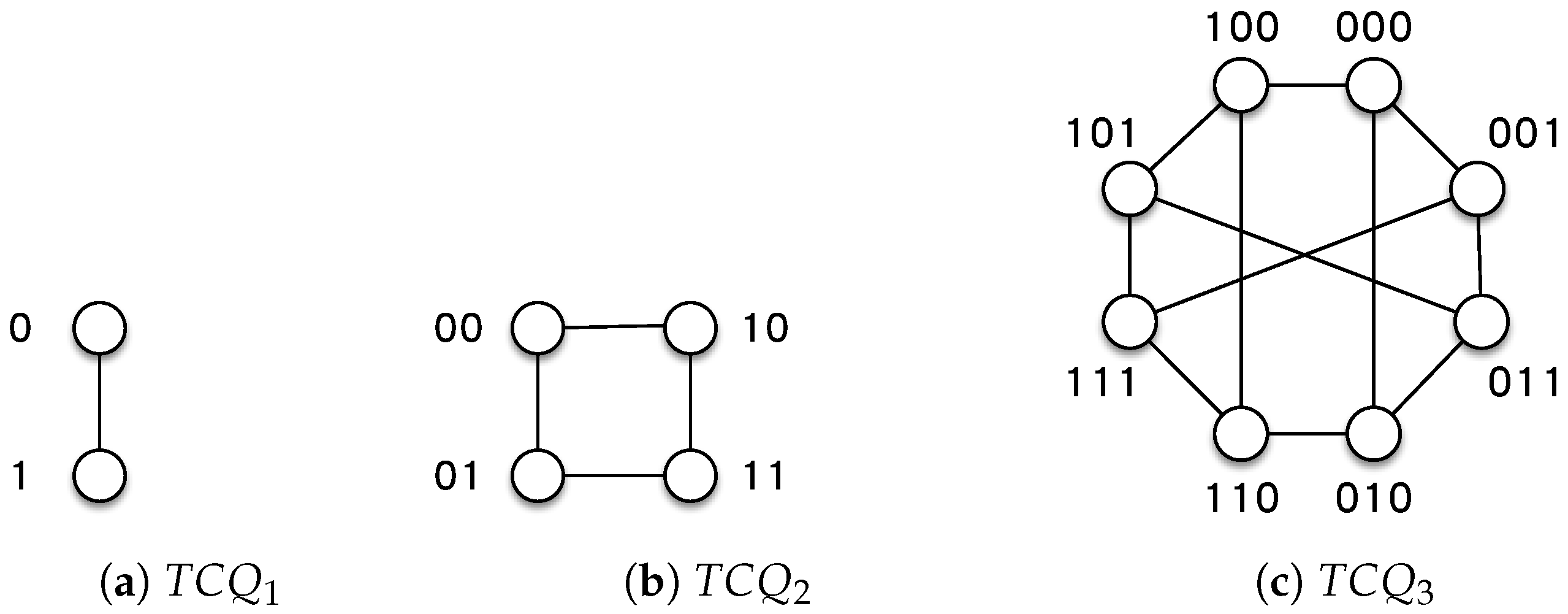
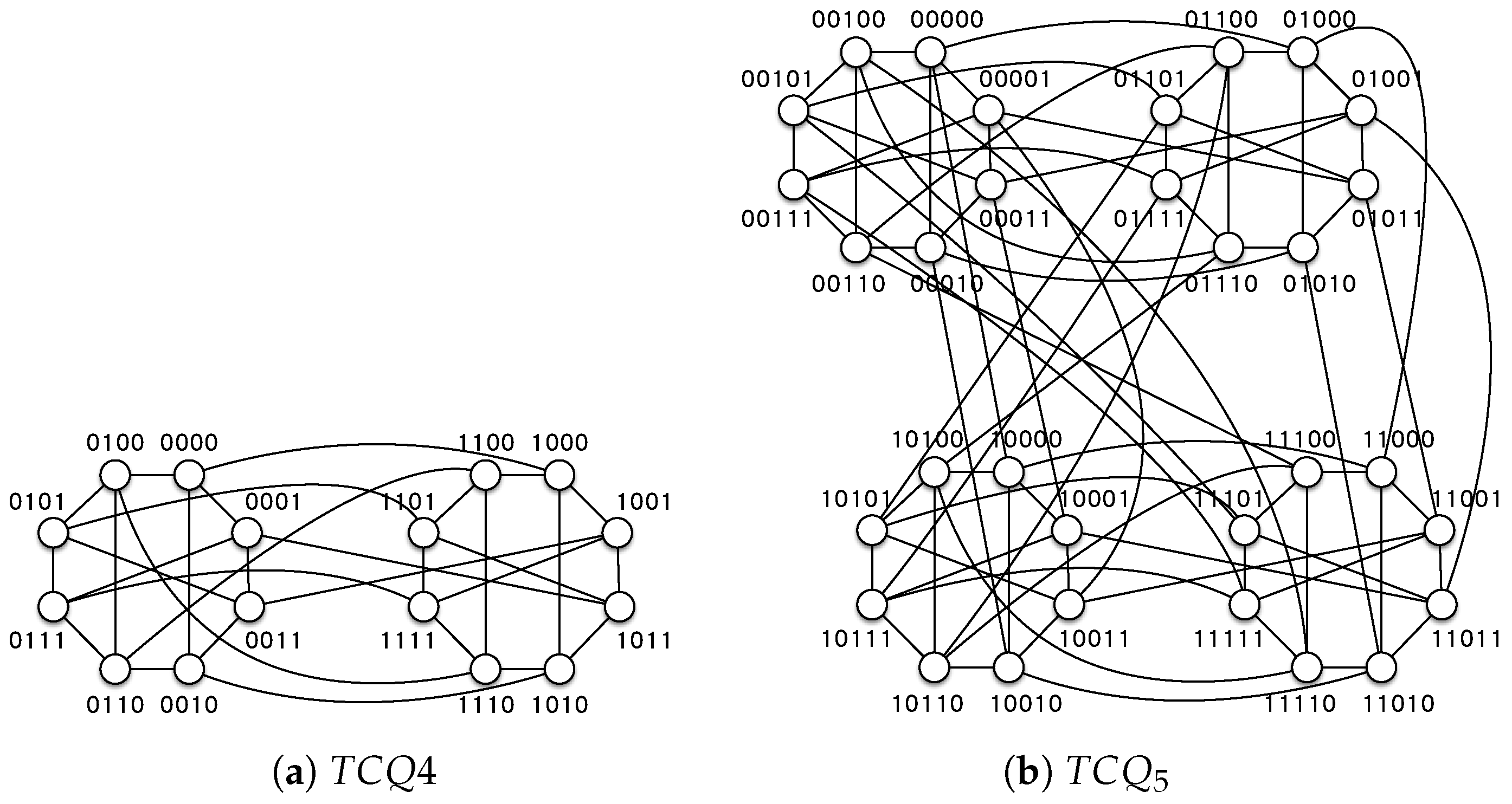
For example, let $v=11011$. Then, $v^0=11010$, $v^1=11001$, $v^2=11101$, $v^3=10001$, and $v^4=01001$. Figure 1 and Figure 2 demonstrate the twisted crossed cubes $TC{Q}_1$, $TC{Q}_2$, $TC{Q}_3$, $TC{Q}_4$, and $TC{Q}_5$.

Figure 1. The twisted crossed cubes $TC{Q}_1$, $TC{Q}_2$, and $TC{Q}_3$.

Figure 2. The twisted crossed cubes $TC{Q}_4$ and $TC{Q}_5$.

Lemma 1. 

$Orb\left(TC{Q}_1\right)=Orb\left(TC{Q}_2\right)$.

Proof. 

According to Figure 1, it is easy to see that $Orb\left(TC{Q}_1\right)=Orb\left(TC{Q}_2\right)=1$. □

2.1. The Upper Bound of $Orb\left(TC{Q}_n\right)$

Let $f_i\left(v\right)$ denote $v_{n-1}\cdots v_{i+1}\overline{v_i}{v}_{i-1}\cdots v_0$ for some $0\le i\le n-1$ for all $v\in V\left(TC{Q}_n\right)$. We use ★ to represent any possible character, i.e., 0 or 1. A function is bijective if and only if it is invertible; that is, a function $f:X\to Y$ is bijective if and only if there is a function $f^{-1}:Y\to X$, the inverse of f, such that each of the two ways for composing the two functions produces the identity function $f^{-1}\left(f\left(x\right)\right)=x$ for each x in X and $f\left(f^{-1}\left(y\right)\right)=y$ for each y in Y.

According to the definition of automorphisms, to prove that $f_i\left(v\right)$ for some i, is an automorphism of $TC{Q}_n$, we need to show that for every edge, $uv\in E\left(TC{Q}_n\right)$ if and only if there exists an edge $\varphi \left(u\right)\varphi \left(v\right)\in E\left(TC{Q}_n\right)$. Since $f_i\left(v\right)$ (=$f_i^{-1}\left(v\right)$) is bijective, it suffices to focus on one direction of the proof.

Lemma 2. 

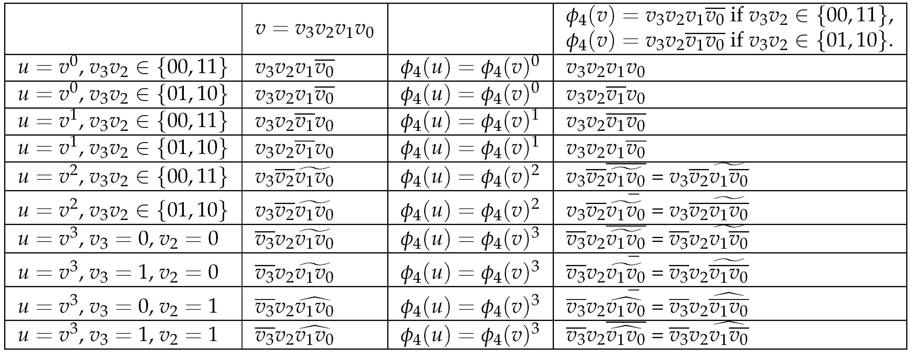
For any n, the function $\varphi \left(v\right)=f_{n-1}\left(v\right)$ for all vertices $v\in V\left(TC{Q}_n\right)$ is an automorphism of $TC{Q}_n$.

Proof. 

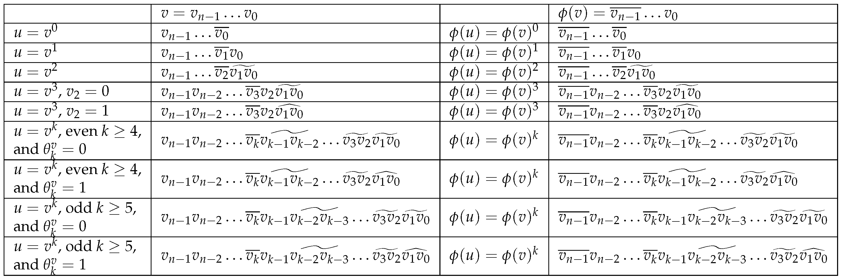
Let $v=v_{n-1}{v}_{n-2}\dots v_1{v}_0$. All possible vertices u and $\varphi \left(u\right)$, corresponding to v and $\varphi \left(v\right)$, are depicted in Figure 3. It is straightforward to verify that $\varphi \left(u\right)\varphi \left(v\right)$ forms an edge in $E\left(TC{Q}_n\right)$, thereby confirming the validity of this lemma. □

Figure 3. All possible vertices u and $\varphi \left(u\right)$ with respect to v and $\varphi \left(v\right)$, where $\varphi \left(v\right)=f_{n-1}\left(v\right)$.

Proposition 1. 

$\stackrel{-}{\widetilde{v_1{v}_0}}=\widetilde{\overline{v_1}{v}_0}$ and $\stackrel{-}{\widehat{v_1{v}_0}}=\widehat{\overline{v_1}{v}_0}$.

Lemma 3. 

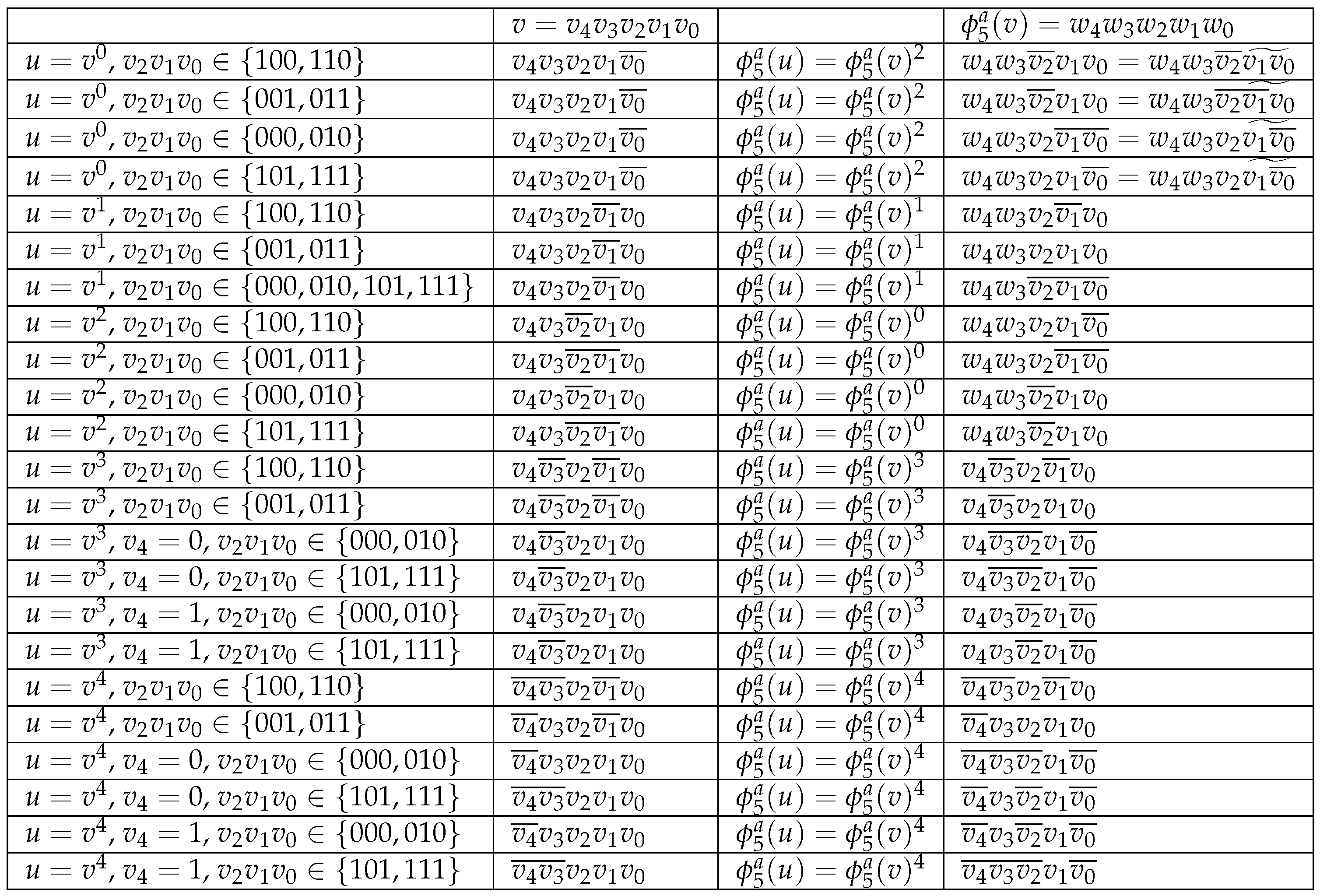
The function $\varphi \left(v\right)=f_h\left(v\right)$, where $h<n-1$ is odd, defines an automorphism of $TC{Q}_n$ for all vertices $v\in V\left(TC{Q}_n\right)$.

Proof. 

Let $v=v_{n-1}{v}_{n-2}\dots v_1{v}_0$. All possible vertices u and $\varphi \left(u\right)$, corresponding to v and $\varphi \left(v\right)$, are depicted in Figure 4. It is straightforward to verify that $\varphi \left(u\right)\varphi \left(v\right)$ forms an edge in $E\left(TC{Q}_n\right)$, thereby confirming the validity of this lemma. □

Figure 4. All possible vertices u and $\varphi \left(u\right)$ with respect to v and $\varphi \left(v\right)$, where $\varphi \left(v\right)=f_h\left(v\right)$ for $h<n-1$ is odd.

Lemma 4. 

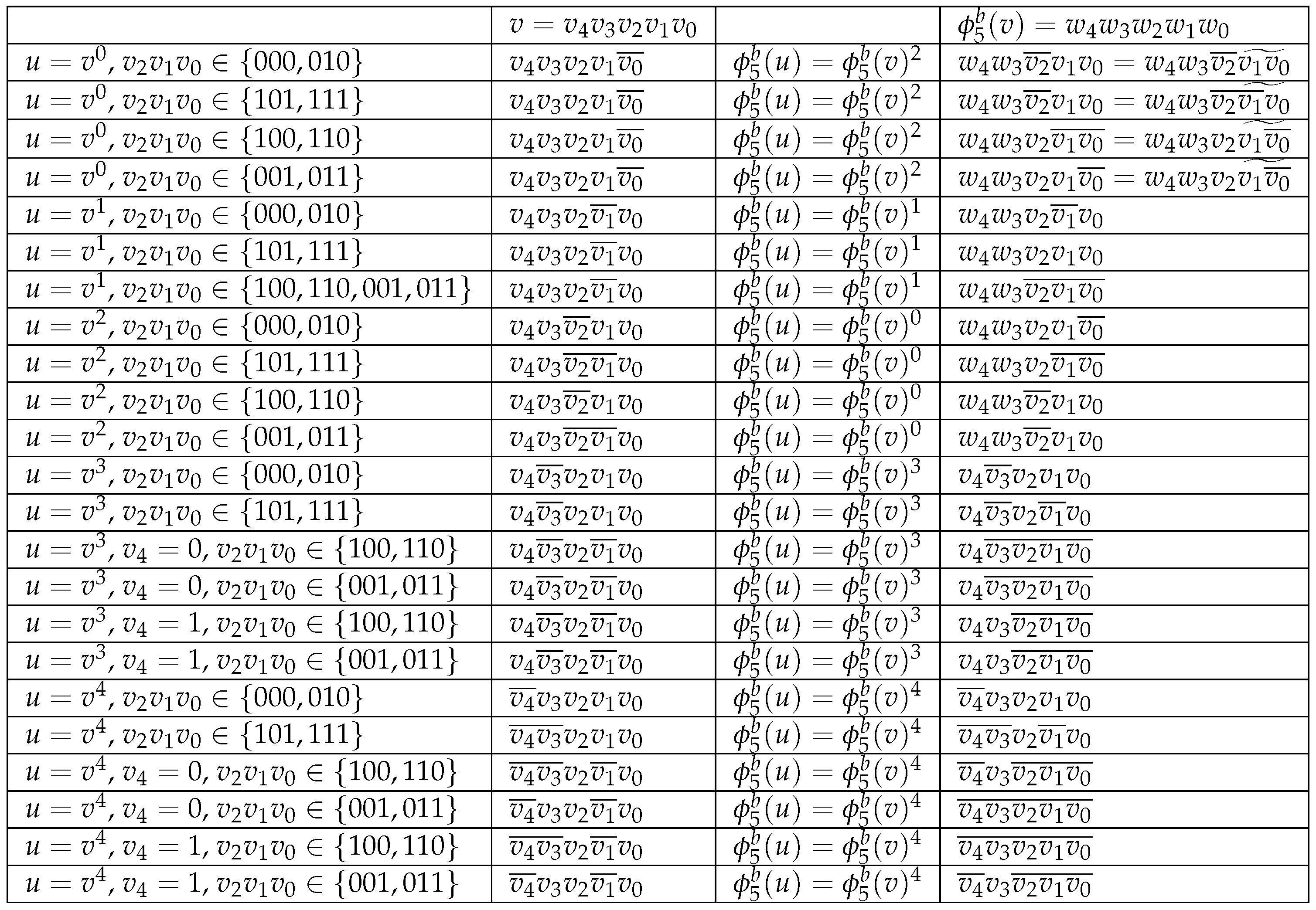
The function $\varphi \left(v\right)=f_h\left(v\right)$, where $h=n-2$ is even, defines an automorphism of $TC{Q}_n$ for all vertices $v\in V\left(TC{Q}_n\right)$.

Proof. 

Let $v=v_{n-1}{v}_{n-2}\dots v_1{v}_0$. All possible vertices u and $\varphi \left(u\right)$, corresponding to v and $\varphi \left(v\right)$, are depicted in Figure 5. □

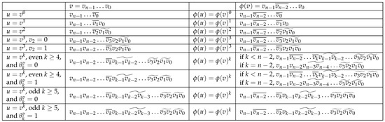
Figure 5. All possible vertices u and $\varphi \left(u\right)$ with respect to v and $\varphi \left(v\right)$, where $\varphi \left(v\right)=f_h\left(v\right)$ for $h=n-2$ is even.

Proposition 2. 

$\overline{\widetilde{v_1{v}_0}}=\widetilde{v_1\overline{v_0}}$, $\stackrel{-}{\widetilde{v_1{v}_0}}=\widetilde{\overline{v_1}\overline{v_0}}$, $\overline{\widehat{v_1{v}_0}}=\widehat{v_1\overline{v_0}}$, and $\stackrel{-}{\widehat{v_1{v}_0}}=\widehat{\overline{v_1}\overline{v_0}}$.

Proof. 

If $v_0=0$, then $\overline{\widetilde{v_1{v}_0}}=\overline{v_1}1=\widetilde{v_1\overline{v_0}}$, $\stackrel{-}{\widetilde{v_1{v}_0}}=v_{1}1=\widetilde{\overline{v_1}\overline{v_0}}$, $\overline{\widehat{v_1{v}_0}}=v_{1}1=\widehat{v_1\overline{v_0}}$, and $\stackrel{-}{\widehat{v_1{v}_0}}=\overline{v_1}1=\widehat{\overline{v_1}\overline{v_0}}$. If $v_0=1$, then $\overline{\widetilde{v_1{v}_0}}=v_{1}0=\widetilde{v_1\overline{v_0}}$, $\stackrel{-}{\widetilde{v_1{v}_0}}=\overline{v_1}0=\widetilde{\overline{v_1}\overline{v_0}}$, $\overline{\widehat{v_1{v}_0}}=\overline{v_1}0=\widehat{v_1\overline{v_0}}$, and $\stackrel{-}{\widehat{v_1{v}_0}}=v_{1}0=\widehat{\overline{v_1}\overline{v_0}}$. □

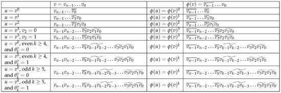
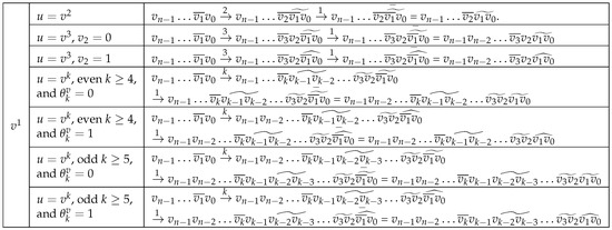
Lemma 5. 

For all vertices $v\in V\left(TC{Q}_3\right)$, let

$$\begin{array}{c}{\varphi }_3\left(v\right)=\left\{\begin{array}{cc}{v}_2{v}_1\overline{v_0}\hfill & if{v}_2=0,\hfill \\ v_2\overline{v_1}\overline{v_0}\hfill & if{v}_2=1.\hfill \end{array}\right.\hfill \end{array}$$

The function ${\varphi }_3\left(v\right)$ defines an automorphism of $TC{Q}_3$.

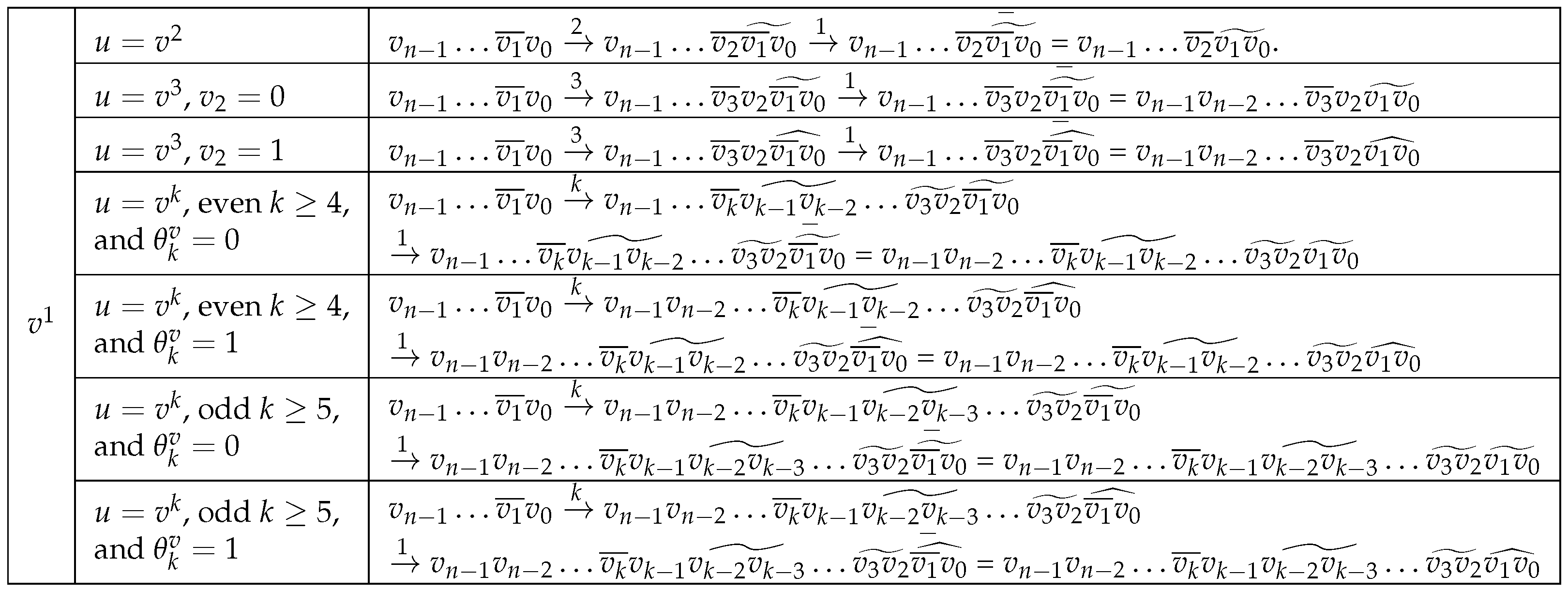
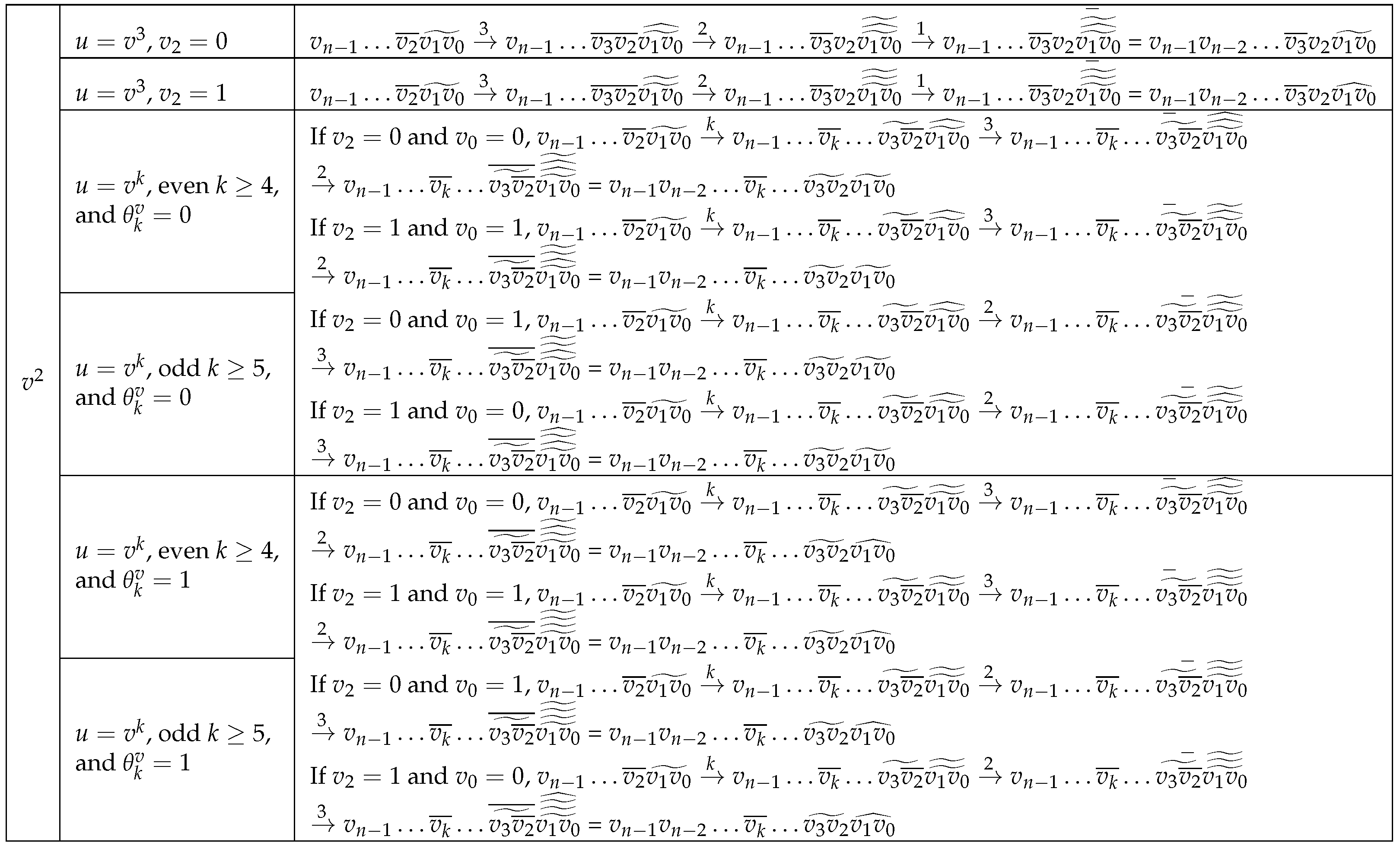
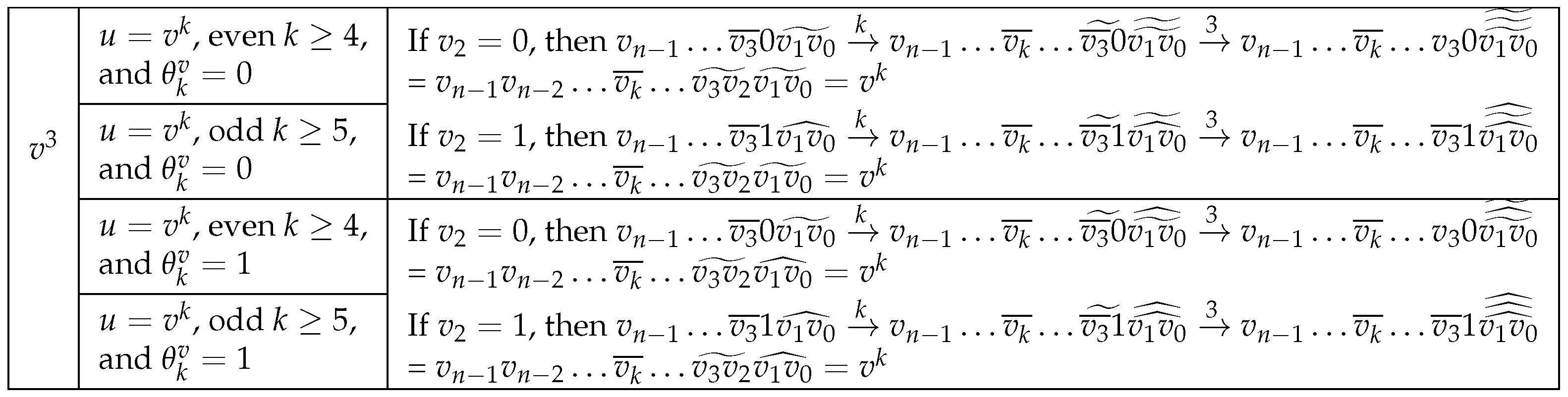
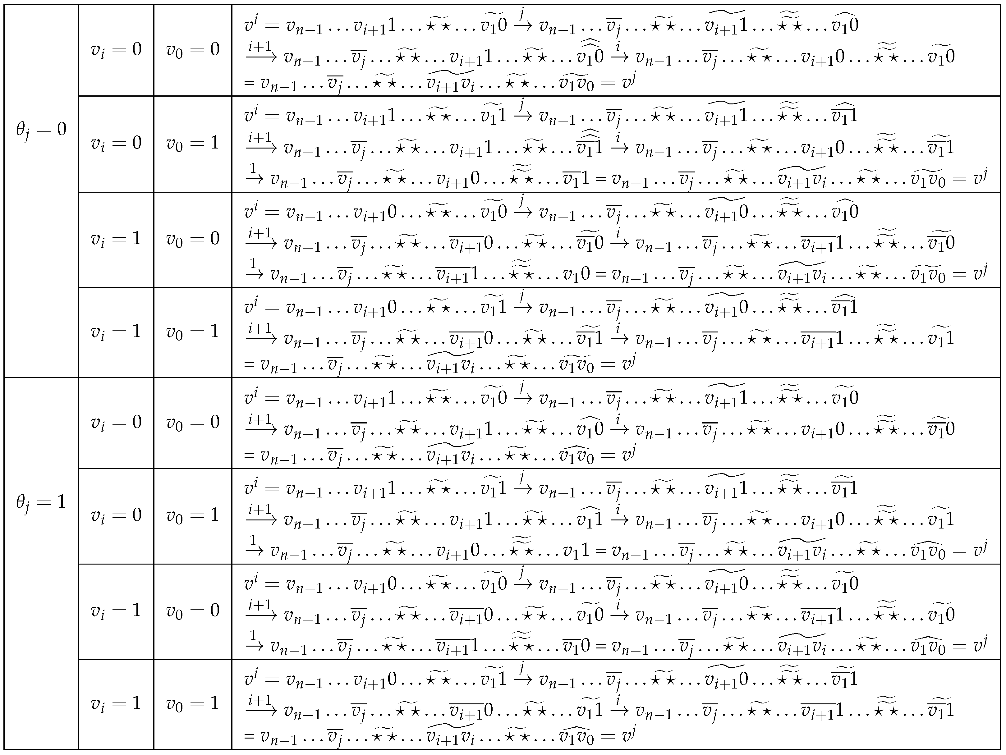
Proof. 

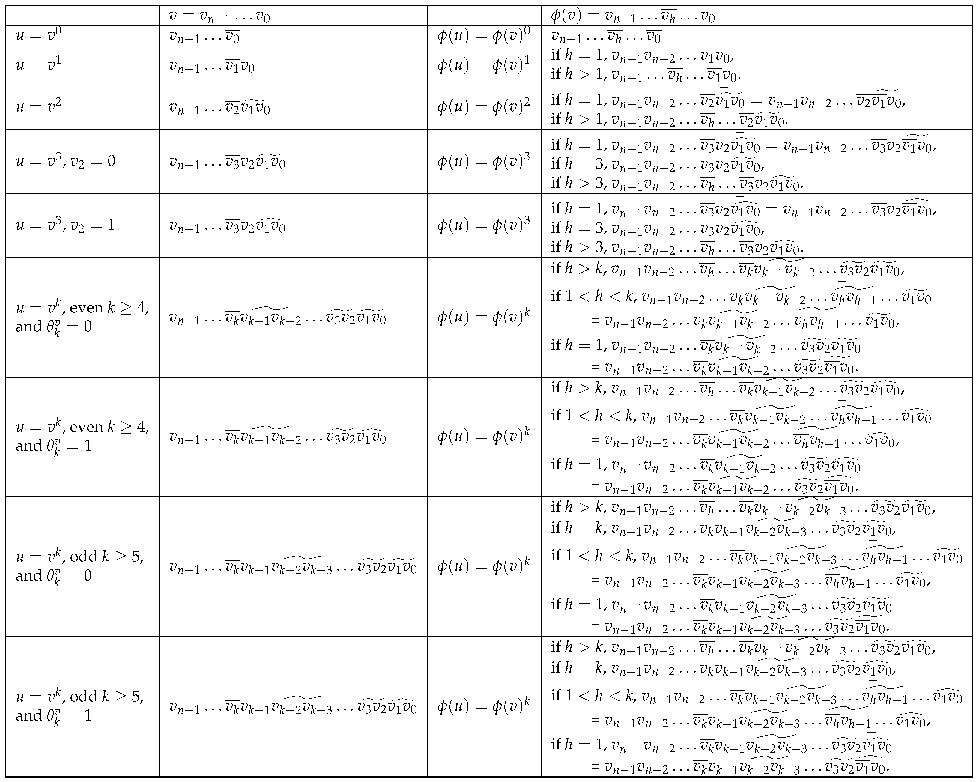
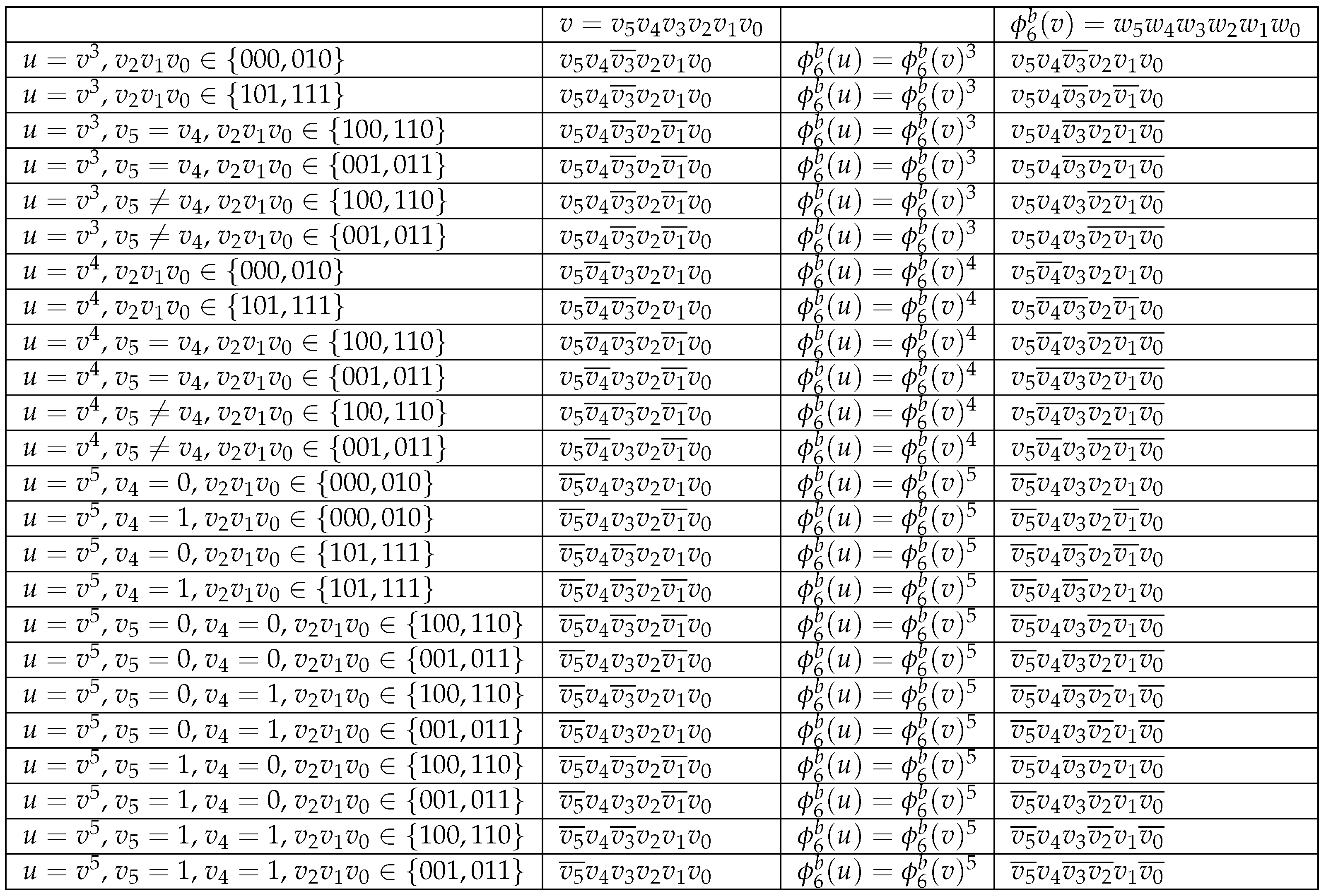
To prove that ${\varphi }_3$ is an automorphism of $TC{Q}_3$, we need to show that for each edge, $uv\in E\left(TC{Q}_3\right)$ if and only if there exists an edge ${\varphi }_3\left(u\right){\varphi }_3\left(v\right)\in E\left(TC{Q}_3\right)$. Since ${\varphi }_3\left(v\right)$ (=${\varphi }_3^{-1}\left(v\right)$) is bijective, it suffices to focus on one direction of the proof. Let $v=v_2{v}_1{v}_0$. All possible vertices u and ${\varphi }_3\left(u\right)$, corresponding to v and ${\varphi }_3\left(v\right)$, are depicted in Figure 6. □

Figure 6. All possible vertices u and ${\varphi }_3\left(u\right)$ with respect to v and ${\varphi }_3\left(v\right)$.

Lemma 6. 

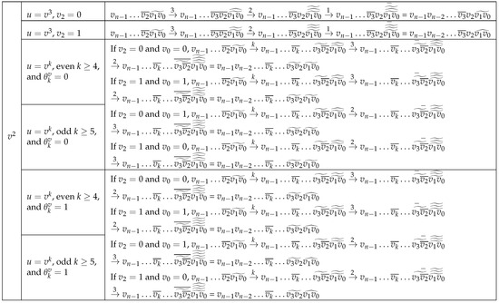
For all vertices $v\in V\left(TC{Q}_4\right)$, let

$$\begin{array}{c}{\varphi }_4\left(v\right)=\left\{\begin{array}{cc}{v}_3{v}_2{v}_1\overline{v_0}\hfill & if{v}_3{v}_2\in \{00,11\},\hfill \\ v_3{v}_2\overline{v_1}\overline{v_0}\hfill & if{v}_3{v}_2\in \{01,10\}.\hfill \end{array}\right.\hfill \end{array}$$

The function ${\varphi }_4\left(v\right)$ defines an automorphism of $TC{Q}_4$.

Proof. 

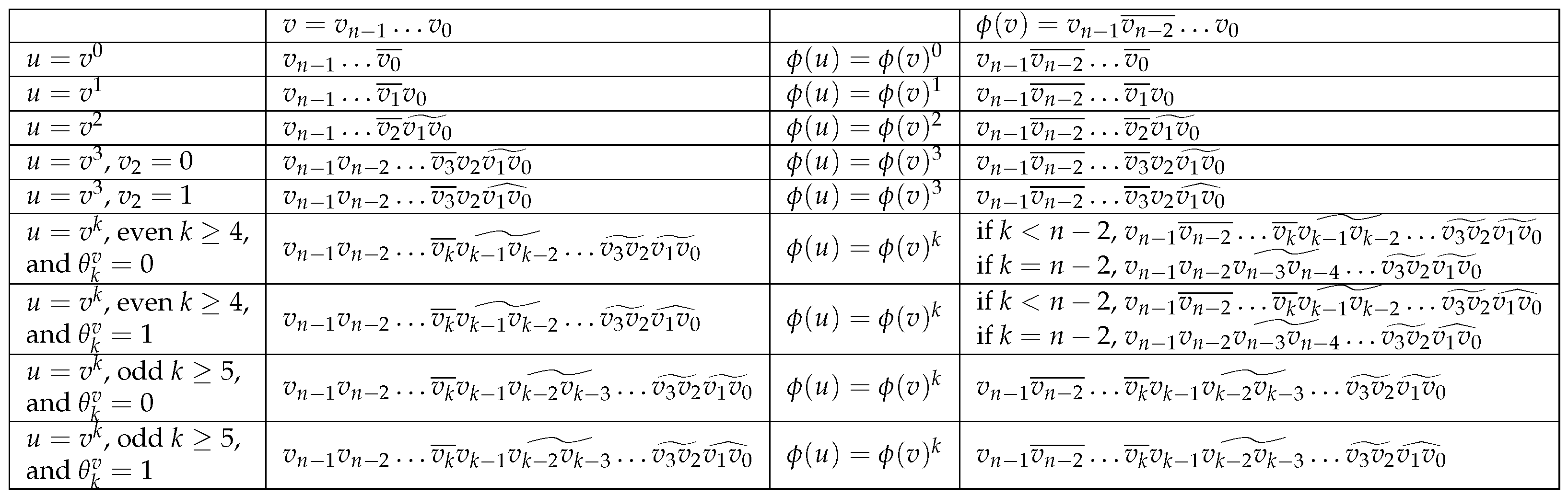
To prove that ${\varphi }_4$ is an automorphism of $TC{Q}_4$, we need to show that for each edge, $uv\in E\left(TC{Q}_4\right)$ if and only if there exists an edge ${\varphi }_4\left(u\right){\varphi }_4\left(v\right)\in E\left(TC{Q}_4\right)$. Since ${\varphi }_4\left(v\right)$ (=${\varphi }_4^{-1}\left(v\right)$) is bijective, it suffices to focus on one direction of the proof. Let $v=v_3{v}_2{v}_1{v}_0$. All possible vertices u and ${\varphi }_4\left(u\right)$, corresponding to v and ${\varphi }_4\left(v\right)$, are depicted in Figure 7. □

Figure 7. All possible vertices u and ${\varphi }_4\left(u\right)$ with respect to v and ${\varphi }_4\left(v\right)$.

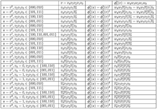
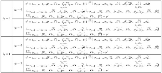
In the following lemmas, we define four automorphism functions of $TC{Q}_5$ and $TC{Q}_6$: ${\varphi }_5^a\left(v\right)$, ${\varphi }_5^b\left(v\right)$, ${\varphi }_6^a\left(v\right)$, and ${\varphi }_6^b\left(v\right)$. These functions are used to map a string ending in 000 to a string ending in 101, and a string ending in 001 to a string ending in 100.

Lemma 7. 

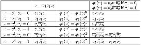
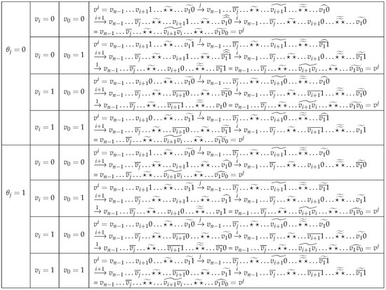
For all vertices $v\in V\left(TC{Q}_5\right)$, let ${\varphi }_5^a\left(v\right)=w_4{w}_3{w}_2{w}_1{w}_0$, where

$$\begin{array}{c}{w}_4{w}_3=\left\{\begin{array}{cc}{v}_4\overline{v_3}\hfill & if{v}_4=1and{v}_2{v}_1{v}_0\in \{000,010,101,111\},\hfill \\ v_4{v}_3\hfill & otherwise,\hfill \end{array}\right.and\hfill \\ w_2{w}_1{w}_0=\left\{\begin{array}{cc}{v}_2{v}_1{v}_0\hfill & if{v}_2{v}_1{v}_0\in \{100,110\},\hfill \\ v_2\overline{v_1}{v}_0\hfill & if{v}_2{v}_1{v}_0\in \{001,011\},\hfill \\ \overline{v_2}{v}_1\overline{v_0}\hfill & if{v}_2{v}_1{v}_0\in \{000,010,101,111\}.\hfill \end{array}\right.\hfill \end{array}$$

The function ${\varphi }_5^a\left(v\right)$ defines an automorphism of $TC{Q}_5$.

Proof. 

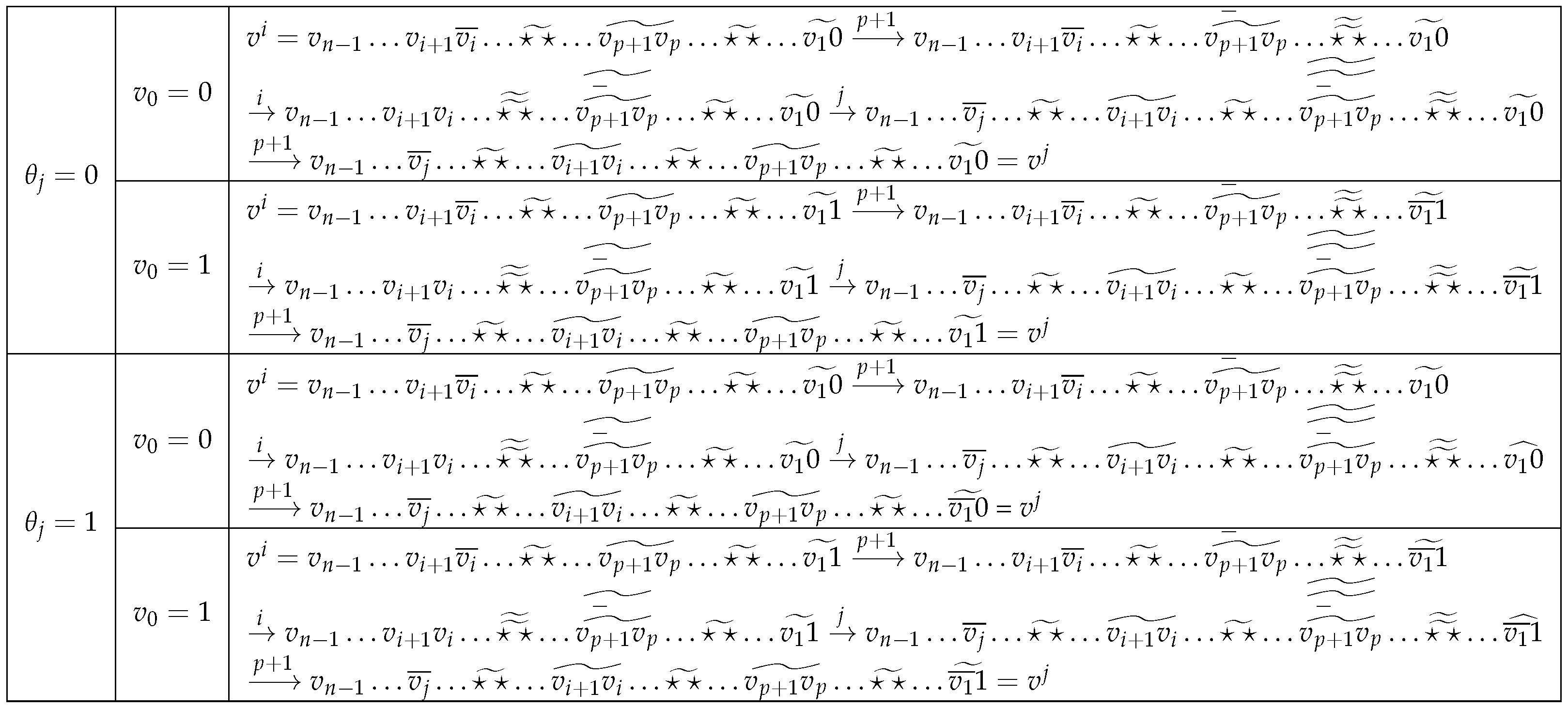
To prove that ${\varphi }_5^a$ is an automorphism of $TC{Q}_5$, we need to show that for each edge, $uv\in E\left(TC{Q}_5\right)$ if and only if there exists an edge ${\varphi }_5^a\left(u\right){\varphi }_5^a\left(v\right)\in E\left(TC{Q}_5\right)$. Since ${\varphi }_5^a\left(v\right)$ (=${\left({\varphi }_5^a\right)}^{-1}\left(v\right)$) is bijective, it suffices to focus on one direction of the proof. Let $v=v_4{v}_3{v}_2{v}_1{v}_0$. All possible vertices u and ${\varphi }_5^a\left(u\right)$, corresponding to v and ${\varphi }_5^a\left(v\right)$, are depicted in Figure 8. □

Figure 8. All possible vertices u and ${\varphi }_5^a\left(u\right)$ with respect to v and ${\varphi }_5^a\left(v\right)$.

Lemma 8. 

For all vertices $v\in V\left(TC{Q}_5\right)$, let ${\varphi }_5^b\left(v\right)=w_4{w}_3{w}_2{w}_1{w}_0$, where

$$\begin{array}{c}{w}_4{w}_3=\left\{\begin{array}{cc}{v}_4\overline{v_3}\hfill & if{v}_4=1and{v}_2{v}_1{v}_0\in \{100,110,001,011\},\hfill \\ v_4{v}_3\hfill & otherwise,\hfill \end{array}\right.and\hfill \\ w_2{w}_1{w}_0=\left\{\begin{array}{cc}{v}_2{v}_1{v}_0\hfill & if{v}_2{v}_1{v}_0\in \{000,010\},\hfill \\ v_2\overline{v_1}{v}_0\hfill & if{v}_2{v}_1{v}_0\in \{101,111\},\hfill \\ \overline{v_2}{v}_1\overline{v_0}\hfill & if{v}_2{v}_1{v}_0\in \{100,110,001,011\}.\hfill \end{array}\right.\hfill \end{array}$$

The function ${\varphi }_5^b\left(v\right)$ defines an automorphism of $TC{Q}_5$.

Proof. 

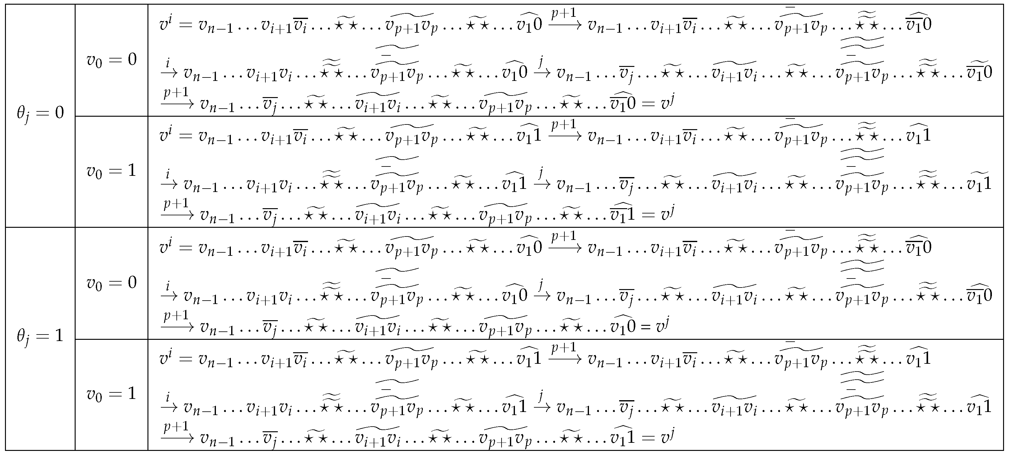
To prove that ${\varphi }_5^b$ is an automorphism of $TC{Q}_5$, we need to show that for each edge, $uv\in E\left(TC{Q}_5\right)$ if and only if there exists an edge ${\varphi }_5^b\left(u\right){\varphi }_5^b\left(v\right)\in E\left(TC{Q}_5\right)$. Since ${\varphi }_5^b\left(v\right)$ (=${\left({\varphi }_5^b\right)}^{-1}\left(v\right)$) is bijective, it suffices to focus on one direction of the proof. Let $v=v_4{v}_3{v}_2{v}_1{v}_0$. All possible vertices u and ${\varphi }_5^b\left(u\right)$, corresponding to v and ${\varphi }_5^b\left(v\right)$, are depicted in Figure 9. □

Figure 9. All possible vertices u and ${\varphi }_5^b\left(u\right)$ with respect to v and ${\varphi }_5^b\left(v\right)$.

Lemma 9. 

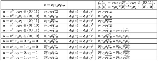
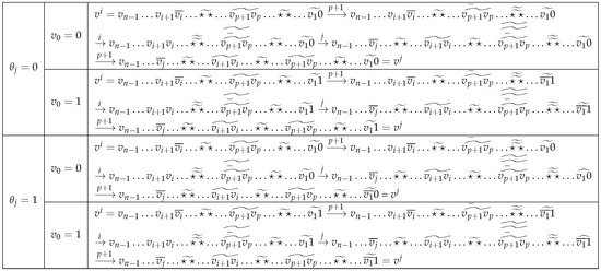
For all vertices $v\in V\left(TC{Q}_6\right)$, let ${\varphi }_6^a\left(v\right)=v_5{w}_4{w}_3{w}_2{w}_1{w}_0$, where

$$\begin{array}{c}{w}_4{w}_3=\left\{\begin{array}{cc}{v}_4\overline{v_3}\hfill & if{v}_5\ne v_{4}and{v}_2{v}_1{v}_0\in \{000,010,101,111\},\hfill \\ v_4{v}_3\hfill & otherwise,\hfill \end{array}\right.and\hfill \\ w_2{w}_1{w}_0=\left\{\begin{array}{cc}{v}_2{v}_1{v}_0\hfill & if{v}_2{v}_1{v}_0\in \{100,110\},\hfill \\ v_2\overline{v_1}{v}_0\hfill & if{v}_2{v}_1{v}_0\in \{001,011\},\hfill \\ \overline{v_2}{v}_1\overline{v_0}\hfill & if{v}_2{v}_1{v}_0\in \{000,010,101,111\}.\hfill \end{array}\right.\hfill \end{array}$$

The function ${\varphi }_6^a\left(v\right)$ defines an automorphism of $TC{Q}_6$.

Proof. 

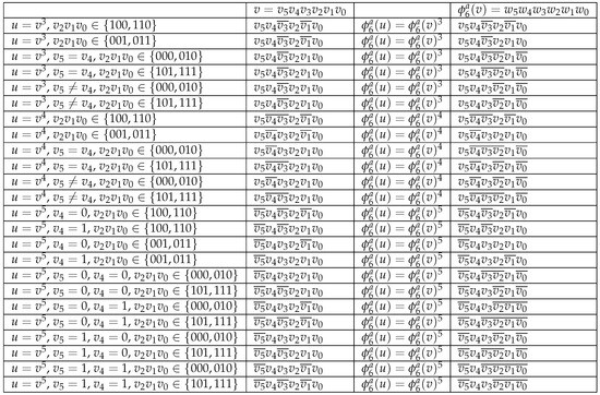
To prove that ${\varphi }_6^a$ is an automorphism of $TC{Q}_6$, we need to show that for each edge, $uv\in E\left(TC{Q}_6\right)$ if and only if there exists an edge ${\varphi }_6^a\left(u\right){\varphi }_6^a\left(v\right)\in E\left(TC{Q}_6\right)$. Since ${\varphi }_6^a\left(v\right)$ (=${\left({\varphi }_6^a\right)}^{-1}\left(v\right)$) is bijective, it suffices to focus on one direction of the proof. Let $v=v_5{v}_4{v}_3{v}_2{v}_1{v}_0$. All possible vertices u and ${\varphi }_6^a\left(u\right)$, corresponding to v and ${\varphi }_6^a\left(v\right)$, are depicted in Figure 10. Note that we omit the parts of $v^0$, $v^1$, and $v^2$ that are analogous to those depicted in Figure 8. □

Figure 10. All possible vertices u and ${\varphi }_6^a\left(u\right)$ with respect to v and ${\varphi }_6^a\left(v\right)$.

Lemma 10. 

For all vertices $v\in V\left(TC{Q}_6\right)$, let ${\varphi }_6^b\left(v\right)=v_5{w}_4{w}_3{w}_2{w}_1{w}_0$, where

$$\begin{array}{c}{w}_4{w}_3=\left\{\begin{array}{cc}{v}_4\overline{v_3}\hfill & if{v}_5\ne v_{4}and{v}_2{v}_1{v}_0\in \{100,110,001,011\},\hfill \\ v_4{v}_3\hfill & otherwise,\hfill \end{array}\right.and\hfill \\ w_2{w}_1{w}_0=\left\{\begin{array}{cc}{v}_2{v}_1{v}_0\hfill & if{v}_2{v}_1{v}_0\in \{000,010\},\hfill \\ v_2\overline{v_1}{v}_0\hfill & if{v}_2{v}_1{v}_0\in \{101,111\},\hfill \\ \overline{v_2}{v}_1\overline{v_0}\hfill & if{v}_2{v}_1{v}_0\in \{100,110,001,011\}.\hfill \end{array}\right.\hfill \end{array}$$

The function ${\varphi }_6^b\left(v\right)$ defines an automorphism of $TC{Q}_6$.

Proof. 

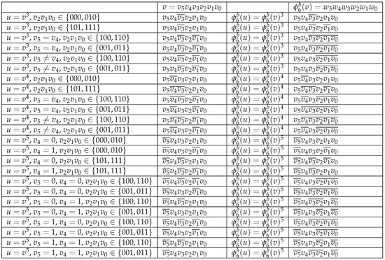
To prove that ${\varphi }_6^b$ is an automorphism of $TC{Q}_6$, we need to show that for each edge, $uv\in E\left(TC{Q}_6\right)$ if and only if there exists an edge ${\varphi }_6^b\left(u\right){\varphi }_6^b\left(v\right)\in E\left(TC{Q}_6\right)$. Since ${\varphi }_6^b\left(v\right)$ (=${\left({\varphi }_6^b\right)}^{-1}\left(v\right)$) is bijective, it suffices to focus on one direction of the proof. Let $v=v_5{v}_4{v}_3{v}_2{v}_1{v}_0$. All possible vertices u and ${\varphi }_6^b\left(u\right)$, corresponding to v and ${\varphi }_6^b\left(v\right)$, are depicted in Figure 11. Similarly, we omit the parts of $v^0$, $v^1$, and $v^2$ that are analogous to those depicted in Figure 9. □

Figure 11. All possible vertices u and ${\varphi }_6^b\left(u\right)$ with respect to v and ${\varphi }_6^b\left(v\right)$.

Lemma 11. 

$Orb\left(TC{Q}_3\right)=Orb\left(TC{Q}_4\right)=1$, $Orb\left(TC{Q}_5\right)=Orb\left(TC{Q}_6\right)\le 2$, and $Orb\left(TC{Q}_n\right)$ ≤ $2^{\lfloor {\displaystyle \frac{n-1}{2}}\rfloor }$ for $n\ge 7$.

Proof. 

According to Lemma 3, vertices $v_{n-1}{v}_{n-2}\dots v_h\dots v_0$ and $v_{n-1}{v}_{n-2}\dots \overline{v_h}\dots v_0$ belong to the same orbit for odd integers $h<n-1$. Applying a single automorphism $\varphi$ halves the number of orbits while doubling the size of each orbit. Lemma 2 implies that vertices $v_{n-1}{v}_{n-2}\dots v_0$ and $\overline{v_{n-1}}{v}_{n-2}\dots v_0$ are in the same orbit. According to Lemma 4, if n is even, vertices $v_{n-1}{v}_{n-2}\dots v_0$ and $v_{n-1}\overline{v_{n-2}}\dots v_0$ are in the same orbit. Therefore, the total number of orbits in $TC{Q}_n$ is at most $2^{\lfloor {\displaystyle \frac{n-1}{2}}\rfloor }$.

Now, we can partition the vertex sets of $TC{Q}_n$ as follows: (1) $V\left(TC{Q}_3\right)$ into two groups, $★★0$ and $★★1$; (2) $V\left(TC{Q}_4\right)$ into two groups, $★★★0$ and $★★★1$; (3) $V\left(TC{Q}_5\right)$ into four groups, $★★0★0$, $★★0★1$, $★★1★0$, and $★★1★1$; and (4) $V\left(TC{Q}_6\right)$ into four groups, $★★★0★0$, $★★★0★1$, $★★★1★0$, and $★★★1★1$. According to Lemmas 5 and 6, vertices 000 and 001, 0000, and 0001 belong to the same orbit. Lemmas 7 and 8 imply that 00000 and 00101, as well as 00001 and 00100, are in the same orbit. Similarly, Lemmas 9 and 10 show that 000000 and 000101, and 000001 and 000100, are in the same orbit. Therefore, $Orb\left(TC{Q}_3\right)=Orb\left(TC{Q}_4\right)=1$ and $Orb\left(TC{Q}_5\right)=Orb\left(TC{Q}_6\right)\le 2$. □

2.2. The Lower Bound of $Orb\left(TC{Q}_n\right)$

For any vertex $v\in V\left(TC{Q}_n\right)$, we discuss the shortest path from $v^i$ to $v^j$ that does not pass through v, where $0\le i<j\le n-1$. Let $d_v(i,j)$ denote the shortest distance between $v^i$ and $v^j$ that does not pass through v.

Proposition 3. 

$\overline{\widetilde{v_1\overline{v_0}}}=\widetilde{v_1{v}_0}$ and $\overline{\widehat{v_1\overline{v_0}}}=\widehat{v_1{v}_0}$.

Proof. 

If $v_0=0$, then $\overline{\widetilde{v_1\overline{v_0}}}=\overline{\overline{v_1}1}=v_{1}0$, $\widetilde{v_1{v}_0}=v_{1}0$, $\overline{\widehat{v_1\overline{v_0}}}$ = $\overline{v_{1}1}=\overline{v_1}0$, and $\widehat{v_1{v}_0}=\overline{v_1}0$. If $v_0=1$, then $\overline{\widetilde{v_1\overline{v_0}}}=\overline{v_{1}0}=\overline{v_1}1$, $\widetilde{v_1{v}_0}=\overline{v_1}1$, $\overline{\widehat{v_1\overline{v_0}}}$=$\overline{\overline{v_1}0}=v_{1}1$, and $\widehat{v_1{v}_0}=v_{1}1$. □

Lemma 12. 

For any vertex $v=v_{n-1}\dots v_0\in V\left(TC{Q}_n\right)$ with $n\ge 5$, $d_v(0,1)=2$ and $d_v(0,j)=3$ for $1<j\le n-1$.

Proof. 

The shortest paths from $v^0$ to $v^j$ for $0<j\le n-1$ are shown in Figure 12. □

Figure 12. The shortest paths from $v^0$ to $v^j$, where $0<j\le n-1$.

Proposition 4. 

$\stackrel{-}{\widetilde{\overline{v_1}{v}_0}}=\widetilde{v_1{v}_0}$ and $\stackrel{-}{\widehat{\overline{v_1}{v}_0}}=\widehat{v_1{v}_0}$.

Proof. 

If $v_0=0$, then $\stackrel{-}{\widetilde{\overline{v_1}{v}_0}}=v_{1}0=\widetilde{v_1{v}_0}$ and $\stackrel{-}{\widehat{\overline{v_1}{v}_0}}$ = $\overline{v_1}0=\widehat{v_1{v}_0}$. If $v_0=1$, then $\stackrel{-}{\widetilde{\overline{v_1}{v}_0}}=\overline{v_1}1=\widetilde{v_1{v}_0}$ and $\stackrel{-}{\widehat{\overline{v_1}{v}_0}}$ = $v_{1}1=\widehat{v_1{v}_0}$. □

Lemma 13. 

For any vertex $v=v_{n-1}\dots v_0\in V\left(TC{Q}_n\right)$ with $n\ge 5$, $d_v(1,j)=2$ for $1<j\le n-1$.

Proof. 

The shortest paths from $v^1$ to $v^j$ for $1<j\le n-1$ are shown in Figure 13. □

Figure 13. The shortest paths from $v^1$ to $v^j$, where $1<j\le n-1$.

Proposition 5. 

$\stackrel{-}{\tilde{\widehat{\widetilde{v_1{v}_0}}}}=\widetilde{v_1{v}_0}$ and $\stackrel{-}{\tilde{\widetilde{\tilde{v_1{v}_0}}}}=\widehat{v_1{v}_0}$.

Proof. 

If $v_0=0$, then $\stackrel{-}{\tilde{\widehat{\widetilde{v_1{v}_0}}}}=\stackrel{-}{\widetilde{\overline{v_1}0}}=v_{1}0=\widetilde{v_1{v}_0}$ and $\stackrel{-}{\tilde{\widetilde{\tilde{v_1{v}_0}}}}$ = $\overline{v_1}0=\widehat{v_1{v}_0}$. If $v_0=1$, then $\stackrel{-}{\tilde{\widehat{\widetilde{v_1{v}_0}}}}=\stackrel{-}{\widetilde{\overline{v_1}1}}=\overline{v_1}1=\widetilde{v_1{v}_0}$ and $\stackrel{-}{\tilde{\widetilde{\tilde{v_1{v}_0}}}}$ = $v_{1}1=\widehat{v_1{v}_0}$. □

Proposition 6. 

$\tilde{\widehat{\widehat{\widetilde{v_{1}0}}}}=\widehat{\tilde{\widehat{\widetilde{v_{1}0}}}}=\widetilde{v_{1}0}$, $\tilde{\tilde{\widehat{\widetilde{v_{1}1}}}}=\widetilde{v_{1}1}$, $\tilde{\widehat{\widetilde{\tilde{v_{1}0}}}}=\widehat{\tilde{\widetilde{\tilde{v_{1}0}}}}=\widehat{v_{1}0}$, and $\tilde{\tilde{\widetilde{\tilde{v_{1}1}}}}=\widehat{v_{1}1}$.

Lemma 14. 

For any vertex $v=v_{n-1}\dots v_0\in V\left(TC{Q}_n\right)$ with $n\ge 5$, $d_v(2,j)=3$ for $2<j\le n-1$.

Proof. 

The shortest paths from $v^2$ to $v^j$ for $2<j\le n-1$ are shown in Figure 14. □

Figure 14. The shortest paths from $v^2$ to $v^j$, where $2<j\le n-1$.

Proposition 7. 

$\widehat{\widetilde{\widehat{v_1{v}_0}}}=\widetilde{v_1{v}_0}$, $\tilde{\widehat{\widetilde{v_1{v}_0}}}=\widehat{v_1{v}_0}$, and $\widehat{\widehat{\widehat{v_1{v}_0}}}=\widehat{v_1{v}_0}$.

Proof. 

If $v_0=0$, then $\widehat{\widetilde{\widehat{v_{1}0}}}=v_{1}0=\widetilde{v_{1}0}$, $\tilde{\widehat{\widetilde{v_{1}0}}}=\overline{v_1}0=\widehat{v_{1}0}$, and $\widehat{\widehat{\widehat{v_{1}0}}}=\overline{v_1}0=\widehat{v_{1}0}$. If $v_0=1$, then $\widehat{\widetilde{\widehat{v_{1}1}}}=\overline{v_1}1=\widetilde{v_{1}1}$, $\tilde{\widehat{\widetilde{v_{1}1}}}=v_{1}1=\widehat{v_{1}1}$, and $\widehat{\widehat{\widehat{v_{1}1}}}=v_{1}1=\widehat{v_{1}1}$. □

Lemma 15. 

For any vertex $v=v_{n-1}\dots v_0\in V\left(TC{Q}_n\right)$ with $n\ge 5$, $d_v(3,j)=2$ for $3<j\le n-1$.

Proof. 

The shortest paths from $v^3$ to $v^j$ for $3<j\le n-1$ are shown in Figure 15. □

Figure 15. The shortest paths from $v^3$ to $v^j$, where $3<j\le n-1$.

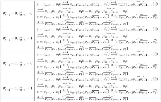
Lemma 16. 

For any vertex $v=v_{n-1}\dots v_0\in V\left(TC{Q}_n\right)$ with $n\ge 7$, even $i\ge 4$, and $i+1<j\le n-1$. Let p be the largest position such that p is even, $v_p=1$, and $0<p<i$. Then,

$$\begin{array}{c}If {\theta }_i=0,d_v(i,j)=\left\{\begin{array}{cc}3\hfill & if\left(\right(v_i=0,v_0=0\left)or\right(v_i=1,v_0=1\left)\right)andpdoesnotexist,\hfill \\ 4\hfill & if\left(\right(v_i=0,v_0=1\left)or\right(v_i=1,v_0=0\left)\right)andpdoesnotexist,\hfill \\ 4\hfill & ifpexist.\hfill \end{array}\right.\hfill \end{array}$$

$$\begin{array}{c}If {\theta }_i=1,d_v(i,j)=4.\hfill \end{array}$$

Proof. 

If ${\theta }_j=0$, $v^j$ = $v_{n-1}\dots \overline{v_j}\dots \widetilde{v_{i+1}{v}_i}\dots \widetilde{v_1{v}_0}$; otherwise, $v^j$ = $v_{n-1}\dots \overline{v_j}\dots \widetilde{v_{i+1}{v}_i}\dots \widehat{v_1{v}_0}$. Assume that ${\theta }_i=0$, $v^i=v_{n-1}\dots v_{i+1}\overline{v_i}\dots \widetilde{v_1{v}_0}$. If no such p exists, then the shortest paths from $v^i$ to $v^j$ are shown in Figure 16; otherwise, please see Figure 17. Note that ★ could be an empty character in this lemma.

Figure 16. The shortest paths from $v^i$ to $v^j$ when ${\theta }_i=0$.

Figure 17. The shortest paths from $v^i$ to $v^j$ when ${\theta }_i=0$.

In the case that ${\theta }_i=1$, p must exist and $v^i=v_{n-1}\dots v_{i+1}\overline{v_i}\dots \widehat{v_1{v}_0}$. The shortest paths from $v^i$ to $v^j$ are shown in Figure 18. □

Figure 18. The shortest paths from $v^i$ to $v^j$ when ${\theta }_i=1$.

Lemma 17. 

For any vertex $v=v_{n-1}\dots v_0\in V\left(TC{Q}_n\right)$ with $n\ge 5$, even $i\ge 4$ and $j=i+1$, $d_v(i,j)=3$.

Proof. 

If ${\theta }_i=0$ and $v_i=0$, then $v^i=v_{n-1}\dots v_j\overline{v_i}\dots \widetilde{v_1{v}_0}$ and $v^j=v_{n-1}\dots \overline{v_j}{v}_i\dots \widetilde{v_1{v}_0}$. The shortest path from $v^i$ to $v^j$ is $v^i=v_{n-1}\dots v_j\overline{v_i}\dots \widetilde{v_1{v}_0}$$\stackrel{j}{\to }$$v_{n-1}\dots \overline{v_j}\overline{v_i}\dots \widehat{\widetilde{v_1{v}_0}}$$\stackrel{i}{\to }$$v_{n-1}\dots \overline{v_j}{v}_i\dots \tilde{\widehat{\widetilde{v_1{v}_0}}}$$\stackrel{1}{\to }$$v_{n-1}\dots \overline{v_j}{v}_i\dots \stackrel{-}{\tilde{\widehat{\widetilde{v_1{v}_0}}}}$ = $v_{n-1}\dots \overline{v_j}{v}_i\dots \widetilde{v_1{v}_0}$ = $v^i$.

If ${\theta }_i=0$ and $v_i=1$, then $v^i=v_{n-1}\dots v_j\overline{v_i}\dots \widetilde{v_1{v}_0}$ and $v^j=v_{n-1}\dots \overline{v_j}{v}_i\dots \widehat{v_1{v}_0}$. The shortest path from $v^i$ to $v^j$ is $v^i=v_{n-1}\dots v_j\overline{v_i}\dots \widetilde{v_1{v}_0}$$\stackrel{j}{\to }$$v_{n-1}\dots \overline{v_j}\overline{v_i}\dots \widetilde{\tilde{v_1{v}_0}}$$\stackrel{i}{\to }$$v_{n-1}\dots \overline{v_j}{v}_i\dots \tilde{\widetilde{\tilde{v_1{v}_0}}}$$\stackrel{1}{\to }$$v_{n-1}\dots \overline{v_j}{v}_i\dots \stackrel{-}{\widetilde{v_1{v}_0}}$ = $v_{n-1}\dots \overline{v_j}{v}_i\dots \widehat{v_1{v}_0}$ = $v^i$.

If ${\theta }_i=1$ and $v_i=0$, then $v^i=v_{n-1}\dots v_j\overline{v_i}\dots \widehat{v_1{v}_0}$ and $v^j=v_{n-1}\dots \overline{v_j}{v}_i\dots \widehat{v_1{v}_0}$. The shortest path from $v^i$ to $v^j$ is $v^i=v_{n-1}\dots v_j\overline{v_i}\dots \widehat{v_1{v}_0}$$\stackrel{j}{\to }$$v_{n-1}\dots \overline{v_j}\overline{v_i}\dots \widetilde{\widehat{v_1{v}_0}}$$\stackrel{i}{\to }$$v_{n-1}\dots \overline{v_j}{v}_i\dots \widehat{\widetilde{\widehat{v_1{v}_0}}}$$\stackrel{1}{\to }$$v_{n-1}\dots \overline{v_j}{v}_i\dots \stackrel{-}{\widehat{\widetilde{\widehat{v_1{v}_0}}}}$ = $v_{n-1}\dots \overline{v_j}{v}_i\dots \widehat{v_1{v}_0}$ = $v^i$.

If ${\theta }_i=1$ and $v_i=1$, then $v^i=v_{n-1}\dots v_j\overline{v_i}\dots \widehat{v_1{v}_0}$ and $v^j=v_{n-1}\dots \overline{v_j}{v}_i\dots \widetilde{v_1{v}_0}$. The shortest path from $v^i$ to $v^j$ is $v^i=v_{n-1}\dots v_j\overline{v_i}\dots \widehat{v_1{v}_0}$$\stackrel{j}{\to }$$v_{n-1}\dots \overline{v_j}\overline{v_i}\dots \widehat{\widehat{v_1{v}_0}}$$\stackrel{i}{\to }$$v_{n-1}\dots \overline{v_j}{v}_i\dots \widehat{\widehat{\widehat{v_1{v}_0}}}$$\stackrel{1}{\to }$$v_{n-1}\dots \overline{v_j}{v}_i\dots \stackrel{-}{\widehat{v_1{v}_0}}$ = $v_{n-1}\dots \overline{v_j}{v}_i\dots \widetilde{v_1{v}_0}$ = $v^i$. □

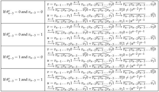
Lemma 18. 

For any vertex $v=v_{n-1}\dots v_0\in V\left(TC{Q}_n\right)$ with $n\ge 5$, i is odd, and $5\le i<j\le n-1$, $d_v(i,j)=2$.

Proof. 

Assume that ${\theta }_i=0$, $v^i=v_{n-1}\dots \overline{v_i}{v}_{i-1}\dots \widetilde{v_1{v}_0}$. If ${\theta }_j=0$, then $v^j$ = $v_{n-1}\dots \overline{v_j}$…$\widetilde{v_i{v}_{i-1}}$$\dots \widetilde{v_1{v}_0}$. The shortest path from $v^i$ to $v^j$ is $v^i=v_{n-1}\dots \overline{v_i}{v}_{i-1}\dots \widetilde{v_1{v}_0}$$\stackrel{j}{\to }$$v_{n-1}\dots \overline{v_j}\dots$$\widetilde{\overline{v_i}{v}_{i-1}}$$\dots \widetilde{\tilde{v_1{v}_0}}$$\stackrel{i}{\to }$$v_{n-1}\dots \overline{v_j}\dots \stackrel{-}{\widetilde{\overline{v_i}{v}_{i-1}}}\dots \widetilde{v_1{v}_0}$ = $v_{n-1}\dots \overline{v_j}\dots \widetilde{v_i{v}_{i-1}}\dots \widetilde{v_1{v}_0}=v^j$. If ${\theta }_j=1$, then $v^j$ = $v_{n-1}\dots \overline{v_j}\dots \widetilde{v_i{v}_{i-1}}\dots \widehat{v_1{v}_0}$. The shortest path from $v^i$ to $v^j$ is $v^i=v_{n-1}\dots \overline{v_i}{v}_{i-1}$…$\widetilde{v_1{v}_0}$$\stackrel{j}{\to }$$v_{n-1}\dots \overline{v_j}\dots \widetilde{\overline{v_i}{v}_{i-1}}\dots \widehat{\widetilde{v_1{v}_0}}$$\stackrel{i}{\to }$$v_{n-1}\dots \overline{v_j}\dots \stackrel{-}{\widetilde{\overline{v_i}{v}_{i-1}}}\dots \widetilde{\overline{v_1}{v}_0}$ = $v_{n-1}\dots \overline{v_j}\dots \widetilde{v_{i+1}{v}_i}$…$\widehat{v_1{v}_0}=v^j$.

In the case that ${\theta }_i=1$, $v^i=v_{n-1}\dots \overline{v_i}{v}_{i-1}\dots \widehat{v_1{v}_0}$. If ${\theta }_j=0$, then $v^j$ = $v_{n-1}\dots \overline{v_j}\dots$$\widetilde{v_i{v}_{i-1}}$$\dots \widetilde{v_1{v}_0}$. The shortest path from $v^i$ to $v^j$ is $v^i=v_{n-1}\dots \overline{v_i}{v}_{i-1}\dots \widehat{v_1{v}_0}$$\stackrel{j}{\to }$$v_{n-1}\dots \overline{v_j}\dots$$\widetilde{\overline{v_i}{v}_{i-1}}$$\dots \widetilde{\widehat{v_1{v}_0}}$$\stackrel{i}{\to }$$v_{n-1}\dots \overline{v_j}\dots \stackrel{-}{\widetilde{\overline{v_i}{v}_{i-1}}}\dots \widehat{\overline{v_1}{v}_0}$ = $v_{n-1}\dots \overline{v_j}\dots \widetilde{v_i{v}_{i-1}}\dots \widetilde{v_1{v}_0}=v^j$. If ${\theta }_j=1$, then $v^j$ = $v_{n-1}\dots \overline{v_j}\dots \widetilde{v_i{v}_{i-1}}\dots \widehat{v_1{v}_0}$. The shortest path from $v^i$ to $v^j$ is $v^i=v_{n-1}\dots \overline{v_i}{v}_{i-1}$…$\widehat{v_1{v}_0}$$\stackrel{j}{\to }$$v_{n-1}\dots \overline{v_j}\dots \widetilde{\overline{v_i}{v}_{i-1}}\dots \widehat{\widehat{v_1{v}_0}}$$\stackrel{i}{\to }$$v_{n-1}\dots \overline{v_j}\dots \stackrel{-}{\widetilde{\overline{v_i}{v}_{i-1}}}\dots \widehat{v_1{v}_0}$ = $v_{n-1}\dots \overline{v_j}\dots \widetilde{v_i{v}_{i-1}}$…$\widehat{v_1{v}_0}=v^j$. □

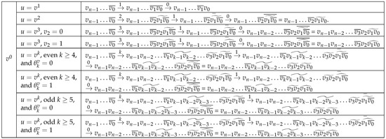
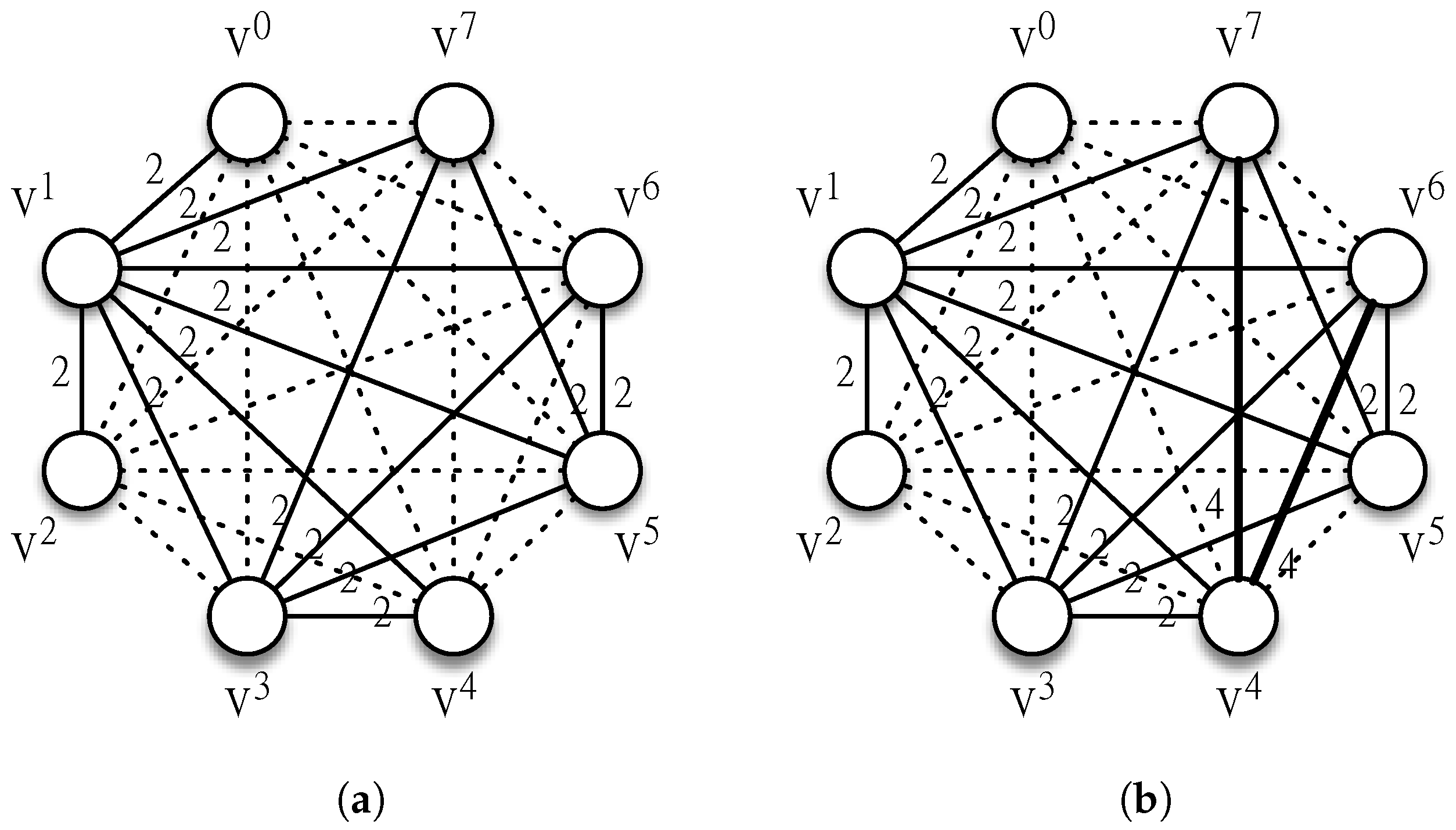
For example, for any vertex $v\in V\left(TC{Q}_7\right)$, Lemma 12 ensures that $d_v(0,1)=2$ and $d_v(0,i)=3$ for $1<j\le n-1$. Lemmas 13–15 imply that $d_v(1,j)=2$ for $1<j\le n-1$, $d_v(2,j)=3$ for $2<j\le n-1$, and $d_v(3,j)=2$ for $3<j\le n-1$. Lemmas 17 and 18 establish that $d_v(i,j)=3$ for even $i\ge 4$ and $j=i+1$, and $d_v(i,j)=2$ for odd i and $5\le i<j\le n-1$. Finally, Lemma 16 distinguishes the shortest paths for even $i\ge 4$ and $i+1<j\le n-1$. As illustrated in Figure 19, we use solid lines, dashed lines, and thick lines to represent distances of 2, 3, and 4, respectively. Figure 19a,b show the shortest paths between the neighbors of vertices 00000000 and 00000100, excluding the vertices themselves.

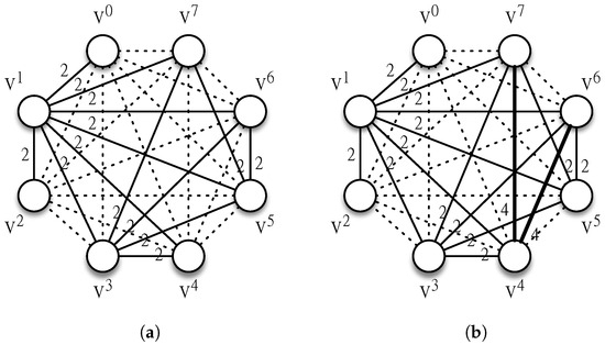
Figure 19. The shortest paths between the neighbors of vertices 00000000 and 00000100, excluding the vertices themselves. (a) The shortest paths between the neighbors of vertex 00000000. (b) The shortest paths between the neighbors of vertex 00000100.

Lemma 19. 

Let ϕ be an automorphism of $TC{Q}_n$ for $n\ge 5$. If $\varphi \left(v\right)=u$ for $v,u\in V\left(TC{Q}_n\right)$, then we have either $\varphi \left(v^0\right)=u^0$ and $\varphi \left(v^2\right)=u^2$ or $\varphi \left(v^0\right)=u^2$ and $\varphi \left(v^2\right)=u^0$.

Proof. 

For any vertex $v\in V\left(TC{Q}_n\right)$, consider the shortest paths between its neighbors. Lemmas 12–18 establish that vertices $v^0$ and $v^2$ are the only neighbors of v with a single 2-distance path and $(n-2)$ 3-distance paths to other neighbors. Thus, this lemma holds. □

Lemma 20. 

Let ϕ be an automorphism of $TC{Q}_n$ for odd $n\ge 5$. If $\varphi \left(v\right)=u$ for $v,u\in V\left(TC{Q}_n\right)$, then we have either $\varphi \left(v^{n-1}\right)=u^{n-1}$ and $\varphi \left(v^{n-2}\right)=u^{n-2}$ or $\varphi \left(v^{n-1}\right)=u^{n-2}$ and $\varphi \left(v^{n-2}\right)=u^{n-1}$.

Proof. 

Since n is odd, Lemmas 13, 15, and 18 imply that there are ${\displaystyle \frac{n-1}{2}}$ neighbors of v at a distance of 2 from both $v^{n-1}$ and $v^{n-2}$, and these neighbors are distinct from the others. Therefore, if $\varphi \left(v\right)=u$ for $v,u\in V\left(TC{Q}_n\right)$, then either $\varphi \left(v^{n-1}\right)=u^{n-1}$ and $\varphi \left(v^{n-2}\right)=u^{n-2}$, or $\varphi \left(v^{n-1}\right)=u^{n-2}$ and $\varphi \left(v^{n-2}\right)=u^{n-1}$. □

Lemma 21. 

Let ϕ be an automorphism of $TC{Q}_n$ for $n\ge 5$. If $\varphi \left(v\right)=u$ for $v,u\in V\left(TC{Q}_n\right)$, then

1. 

$\varphi \left(v^i\right)=u^i$ for i is odd when n is even;

2. 

$\varphi \left(v^i\right)=u^i$ for $i>2$ is even when n is even;

3. 

$\varphi \left(v^i\right)=u^i$ for $i<n-2$ is odd when n is odd;

4. 

$\varphi \left(v^i\right)=u^i$ for $2<i<n-2$ is even when n is odd.

Proof. 

For any vertex $v\in V\left(TC{Q}_n\right)$, consider the shortest paths between the neighbors of v. Lemmas 12 and 13 imply that $n-1$ neighbors of v have a distance of 2 from vertex $v^1$. Lemmas 13 and 15 show that $n-3$ neighbors of v have a distance of 2 from vertex $v^3$. Lemmas 13, 15, and 18 establish that ${\displaystyle \frac{k-1}{2}}+(n-1-k)$ neighbors of v have a distance of 2 from vertex $v^k$ for odd $k>3$. Since all other distances are at least 3, these odd neighbors are distinct. Therefore, if $\varphi \left(v\right)=u$ for $v,u\in V\left(TC{Q}_n\right)$, then $\varphi \left(v^i\right)=u^i$ for all i is odd. Similarly, the numbers of 2-distance paths from $v^i$, for even $i>2$, to other neighbors are distinct. □

Proposition 8. 

$\stackrel{-}{\widetilde{v_{i+1}\overline{v_i}}}=\widetilde{\overline{v_{i+1}}{v}_i}$

Proof. 

If $v_i=0$, then $\stackrel{-}{\widetilde{v_{i+1}\overline{v_i}}}=\overline{v_{i+1}}0=\widetilde{\overline{v_{i+1}}{v}_i}$; otherwise, $\stackrel{-}{\widetilde{v_{i+1}\overline{v_i}}}=v_{i+1}1=\widetilde{\overline{v_{i+1}}{v}_i}$. □

Lemma 22. 

For $n\ge 5$, vertices $v=v_{n-1}\dots v_{1}0$ and $u=v_{n-1}\dots v_{1}1$ are in different orbits.

Proof. 

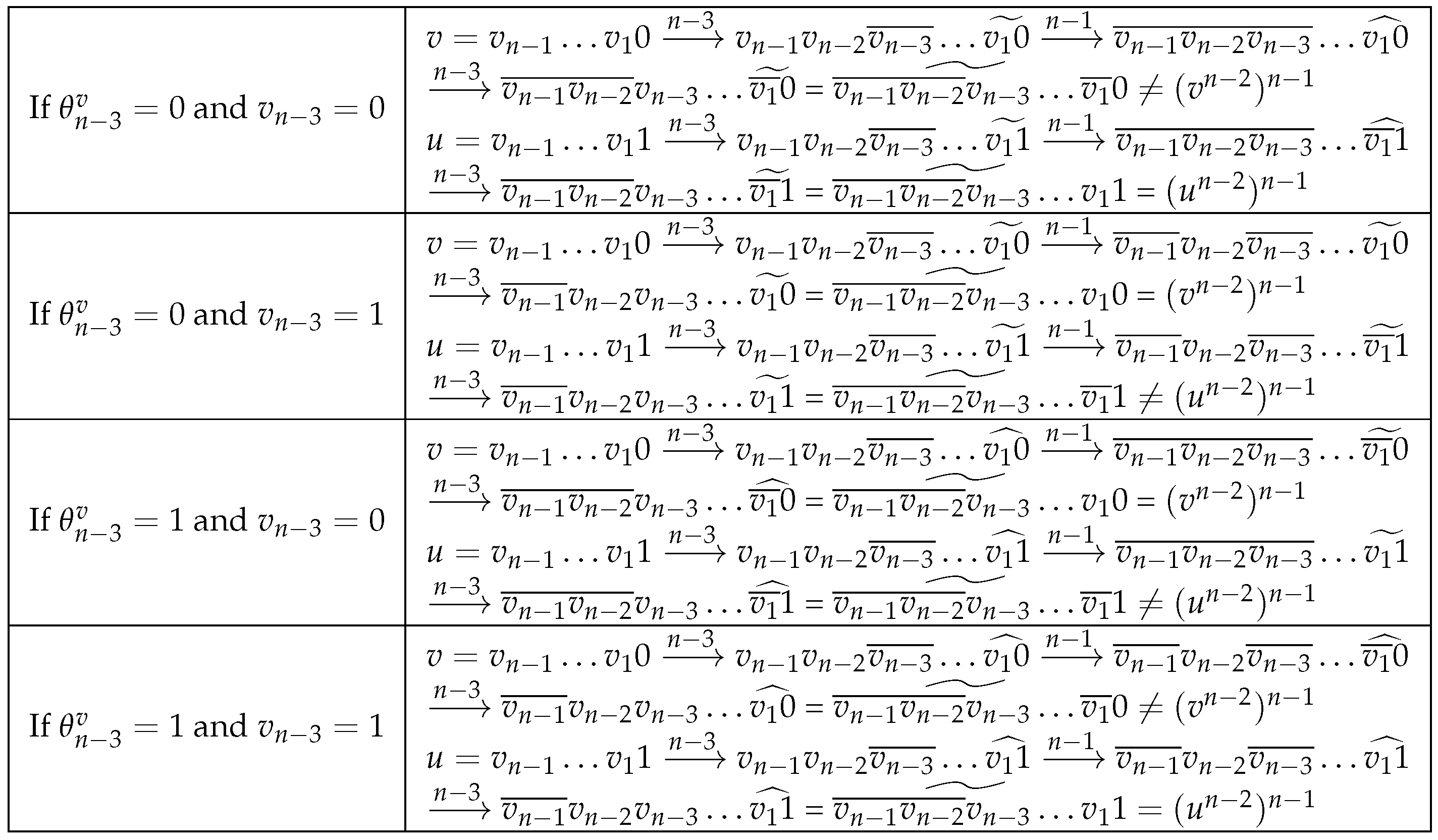
Assume there exists an automorphism $\varphi$ such that $\varphi \left(v\right)=u$. Lemma 21 implies that $\varphi \left({\left(v^{n-3}\right)}^{n-1}\right)={\left(u^{n-3}\right)}^{n-1}$ and $\varphi \left({\left({\left(v^{n-4}\right)}^{n-1}\right)}^{n-4}\right)={\left({\left(u^{n-4}\right)}^{n-1}\right)}^{n-4}$ for even n, and either $\varphi \left({\left(v^{n-2}\right)}^{n-1}\right)={\left(u^{n-2}\right)}^{n-1}$ and $\varphi \left({\left({\left(v^{n-3}\right)}^{n-1}\right)}^{n-3}\right)={\left({\left(u^{n-3}\right)}^{n-1}\right)}^{n-3}$ or $\varphi \left({\left(v^{n-2}\right)}^{n-1}\right)={\left(u^{n-1}\right)}^{n-2}$ and $\varphi \left({\left({\left(v^{n-3}\right)}^{n-1}\right)}^{n-3}\right)={\left({\left(u^{n-3}\right)}^{n-2}\right)}^{n-3}$ for odd n.

For even n, we have ${\left(v^{n-3}\right)}^{n-1}$ = $\overline{v_{n-1}}{v}_{n-2}\widetilde{\overline{v_{n-3}}{v}_{n-4}}\dots v_{1}0$ and ${\left(u^{n-3}\right)}^{n-1}$ = $\overline{v_{n-1}}{v}_{n-2}$$\widetilde{\overline{v_{n-3}}{v}_{n-4}}\dots v_{1}1$ when ${\theta }_{n-1}^v={\theta }_{n-4}^v\oplus v_{n-4}$, and ${\left(v^{n-3}\right)}^{n-1}$ = $\overline{v_{n-1}}{v}_{n-2}\widetilde{\overline{v_{n-3}}{v}_{n-4}}\dots \overline{v_1}0$ and ${\left(u^{n-3}\right)}^{n-1}$ = $\overline{v_{n-1}}{v}_{n-2}\widetilde{\overline{v_{n-3}}{v}_{n-4}}\dots \overline{v_1}1$ when ${\theta }_{n-1}^v\ne {\theta }_{n-4}^v\oplus v_{n-4}$. Figure 20 shows that ${\left({\left(u^{n-4}\right)}^{n-1}\right)}^{n-4}={\left(u^{n-3}\right)}^{n-1}$ = $\varphi \left({\left(v^{n-3}\right)}^{n-1}\right)$≠$\varphi \left({\left({\left(v^{n-4}\right)}^{n-1}\right)}^{n-4}\right)$ when $({\theta }_{n-1}^v,{\theta }_{n-4}^v,v_{n-4})$$\in \{000,011,100,111\}$ and $\varphi \left({\left({\left(v^{n-4}\right)}^{n-1}\right)}^{n-4}\right)$ = $\varphi \left({\left(v^{n-3}\right)}^{n-1}\right)$ = ${\left(u^{n-3}\right)}^{n-1}$≠${\left({\left(u^{n-4}\right)}^{n-1}\right)}^{n-4}$ when $({\theta }_{n-1}^v,{\theta }_{n-4}^v,v_{n-4})\in \{001,010,101,110\}$.

Figure 20. ${\left({\left(v^{n-4}\right)}^{n-1}\right)}^{n-4}$ and ${\left({\left(u^{n-4}\right)}^{n-1}\right)}^{n-4}$.

For odd n, since ${\left(u^{n-1}\right)}^{n-2}$≠${\left({\left(u^{n-3}\right)}^{n-2}\right)}^{n-3}$, we consider the case that $\varphi \left({\left(v^{n-2}\right)}^{n-1}\right)$=${\left(u^{n-2}\right)}^{n-1}$ and $\varphi \left({\left({\left(v^{n-3}\right)}^{n-1}\right)}^{n-3}\right)$ = ${\left({\left(u^{n-3}\right)}^{n-1}\right)}^{n-3}$. We have ${\left(v^{n-2}\right)}^{n-1}$ = $\overline{v_{n-1}}$$\widetilde{\overline{v_{n-2}}{v}_{n-3}}$$\dots v_{1}0$ and ${\left(u^{n-2}\right)}^{n-1}$ = $\overline{v_{n-1}}\widetilde{\overline{v_{n-2}}{v}_{n-3}}\dots v_{1}1$. Figure 21 represents $\varphi \left({\left({\left(v^{n-3}\right)}^{n-1}\right)}^{n-3}\right)$ = $\varphi \left({\left(v^{n-2}\right)}^{n-1}\right)$ = ${\left(u^{n-2}\right)}^{n-1}$≠${\left({\left(u^{n-3}\right)}^{n-1}\right)}^{n-3}$ when ${\theta }_{n-3}^v\oplus v_{n-3}=1$ and ${\left({\left(u^{n-3}\right)}^{n-1}\right)}^{n-3}$ = ${\left(u^{n-2}\right)}^{n-1}$ = $\varphi \left({\left(v^{n-2}\right)}^{n-1}\right)$≠$\varphi \left({\left({\left(v^{n-3}\right)}^{n-1}\right)}^{n-3}\right)$ when ${\theta }_{n-3}^v\oplus v_{n-3}=0$. These contradictions imply that no automorphism $\varphi$ can map v to u, and therefore, vertices v and u are in different orbits. □

Figure 21. ${\left({\left(v^{n-3}\right)}^{n-2}\right)}^{n-3}$ and ${\left({\left(u^{n-3}\right)}^{n-2}\right)}^{n-3}$.

Lemma 23. 

For $n\ge 7$, vertices $v=v_{n-1}\dots 0v_{3}0v_{1}1$ and $u=v_{n-1}\dots 0v_{3}1v_{1}1$ are in different orbits.

Proof. 

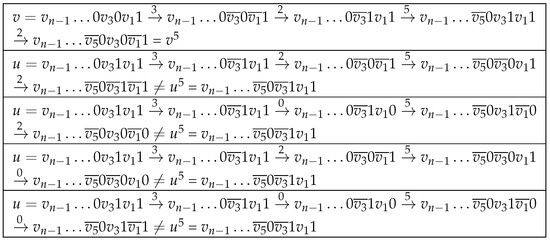
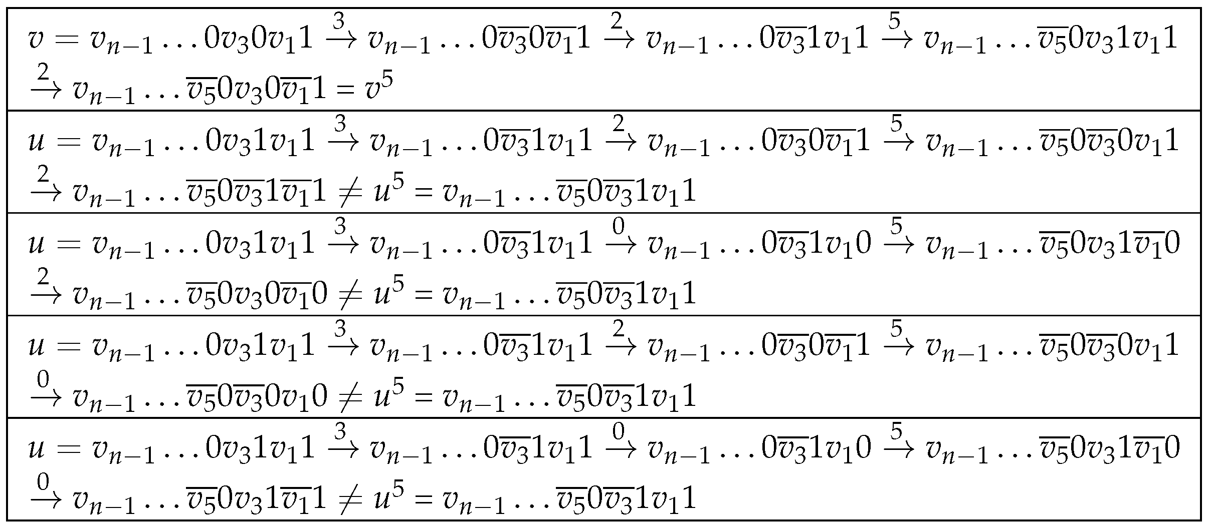
Assume there exists an automorphism $\varphi$ such that $\varphi \left(v\right)=u$. Lemma 21 implies that $\varphi \left(v^3\right)=u^3$ and $\varphi \left(v^5\right)=u^5$. Applying Lemma 19, we determine that $\varphi \left({\left({\left({\left(v^3\right)}^2\right)}^5\right)}^2\right)$ is equal to ${\left({\left({\left(u^3\right)}^2\right)}^5\right)}^2$, ${\left({\left({\left(u^3\right)}^0\right)}^5\right)}^2$, ${\left({\left({\left(u^3\right)}^2\right)}^5\right)}^0$, or ${\left({\left({\left(u^3\right)}^0\right)}^5\right)}^0$. Figure 22 represents ${\left({\left({\left(v^3\right)}^2\right)}^5\right)}^2$, ${\left({\left({\left(u^3\right)}^2\right)}^5\right)}^2$, ${\left({\left({\left(u^3\right)}^0\right)}^5\right)}^2$, ${\left({\left({\left(u^3\right)}^2\right)}^5\right)}^0$, and ${\left({\left({\left(u^3\right)}^0\right)}^5\right)}^0$. Thus, $\varphi \left({\left({\left({\left(v^3\right)}^2\right)}^5\right)}^2\right)=\varphi \left(v^5\right)=u^5\notin \{{\left({\left({\left(u^3\right)}^2\right)}^5\right)}^2,{\left({\left({\left(u^3\right)}^0\right)}^5\right)}^2,{\left({\left({\left(u^3\right)}^2\right)}^5\right)}^0,{\left({\left({\left(u^3\right)}^0\right)}^5\right)}^0\}$. Therefore, vertices $v=v_{n-1}\dots 0v_{3}0v_{1}1$ and $u=v_{n-1}\dots 0v_{3}1v_{1}1$ are in different orbits. □

Figure 22. ${\left({\left({\left(v^3\right)}^2\right)}^5\right)}^2$, ${\left({\left({\left(u^3\right)}^2\right)}^5\right)}^2$, ${\left({\left({\left(u^3\right)}^0\right)}^5\right)}^2$, ${\left({\left({\left(u^3\right)}^2\right)}^5\right)}^0$, and ${\left({\left({\left(u^3\right)}^0\right)}^5\right)}^0$.

Lemma 24. 

For $n\ge 7$, vertices $v=v_{n-1}\dots 1v_{3}0v_{1}0$ and $u=v_{n-1}\dots 1v_{3}1v_{1}0$ are in different orbits.

Proof. 

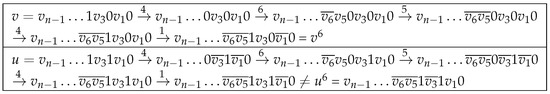
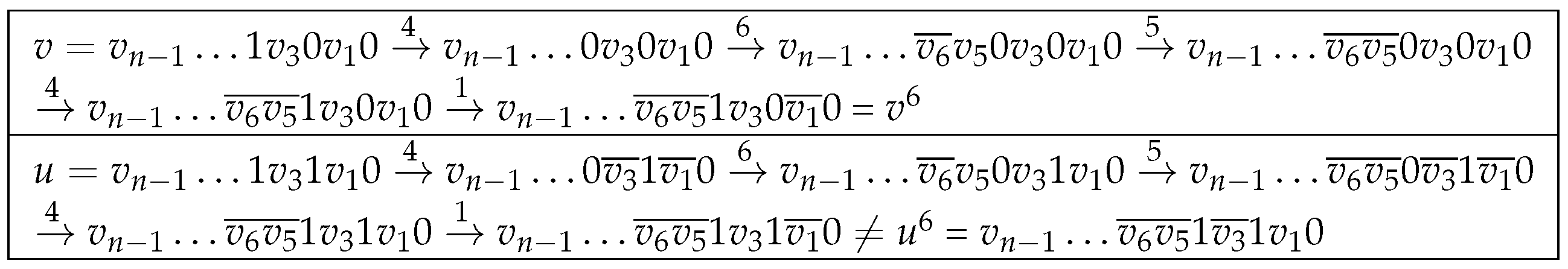
Assume there exists an automorphism $\varphi$ such that $\varphi \left(v\right)=u$. Lemma 21 implies that $\varphi \left(v^6\right)=u^6$ and $\varphi \left({\left({\left({\left({\left(v^4\right)}^6\right)}^5\right)}^4\right)}^1\right)={\left({\left({\left({\left(u^4\right)}^6\right)}^5\right)}^4\right)}^1$. Figure 23 represents ${\left({\left({\left({\left(v^4\right)}^6\right)}^5\right)}^4\right)}^1$ and ${\left({\left({\left({\left(u^4\right)}^6\right)}^5\right)}^4\right)}^1$. Thus, $\varphi \left({\left({\left({\left({\left(v^4\right)}^6\right)}^5\right)}^4\right)}^1\right)=\varphi \left(v^6\right)=u^6\ne {\left({\left({\left({\left(u^4\right)}^6\right)}^5\right)}^4\right)}^1$. Therefore, vertices $v=v_{n-1}\dots 1v_{3}0v_{1}0$ and $u=v_{n-1}\dots 1v_{3}1v_{1}0$ are in different orbits. □

Figure 23. ${\left({\left({\left({\left(v^4\right)}^6\right)}^5\right)}^4\right)}^1$ and ${\left({\left({\left({\left(u^4\right)}^6\right)}^5\right)}^4\right)}^1$.

Lemma 25. 

For $n\ge 7$, vertices $v=v_{n-1}\dots v_{3}0v_1{v}_0$ and $u=v_{n-1}\dots v_{3}1v_1{v}_0$ are in different orbits.

Proof. 

We consider the following four cases: (1) $v_4=0$ and $v_0=0$, (2) $v_4=0$ and $v_0=1$, (3) $v_4=1$ and $v_0=0$, and (4) $v_4=1$ and $v_0=1$. According to Lemma 16, $d_v(4,6)=3$ and $d_u(4,6)=4$ in case 1, $d_v(4,6)=4$ and $d_u(4,6)=4$ in case 2, $d_v(4,6)=4$ and $d_u(4,6)=4$ in case 3, and $d_v(4,6)=3$ and $d_u(4,6)=4$ in case 4. Since $d_v(4,6)\ne d_u(4,6)$ in cases 1 and 4, vertices v and u are in different orbits. According to Lemmas 23 and 24, vertices v and u are in different orbits in cases 2 and 3, respectively. □

Lemma 26. 

For $n\ge 7$, vertices $v=v_{n-1}\dots v_{j+1}0v_{j-1}\dots v_0$ and $u=v_{n-1}\dots v_{j+1}1v_{j-1}\dots v_0$ are in different orbits, where $2<j<n-2$ is even.

Proof. 

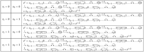
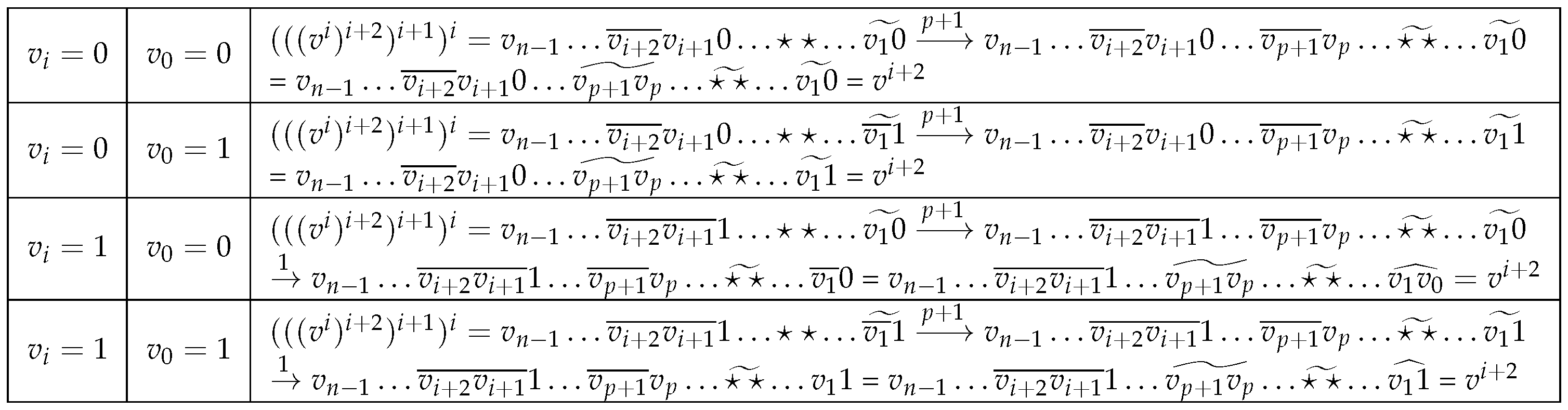
Let p be the largest even position such that $0<p<i$ and $v_p=1$. If no such p exists, Lemma 16 implies that $d_v(i,i+2)\ne d_u(i,i+2)$, and therefore, vertices v and u are in different orbits. Conversely, Lemma 21 implies that $\varphi \left({\left({\left({\left({\left(v^i\right)}^{i+2}\right)}^{i+1}\right)}^i\right)}^{p+1}\right)={\left({\left({\left({\left(u^i\right)}^{i+2}\right)}^{i+1}\right)}^i\right)}^{p+1}$.

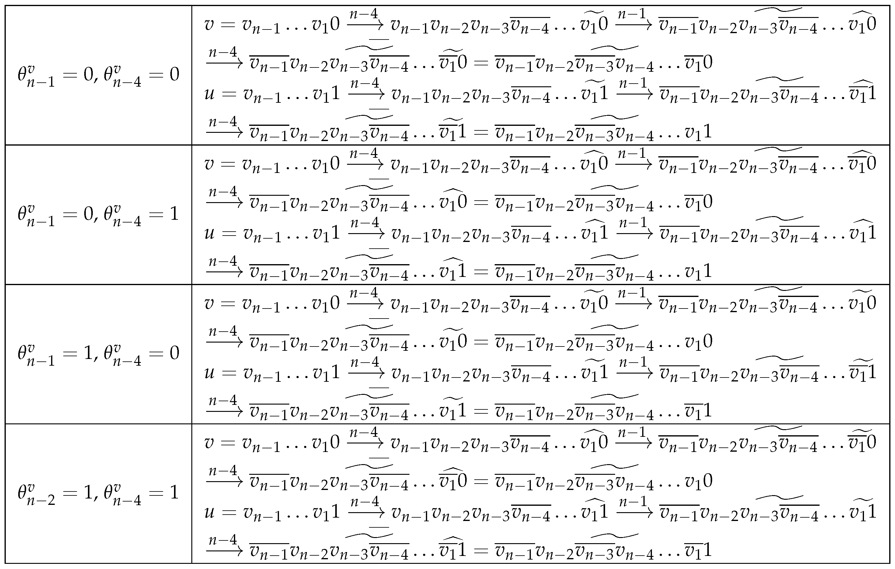
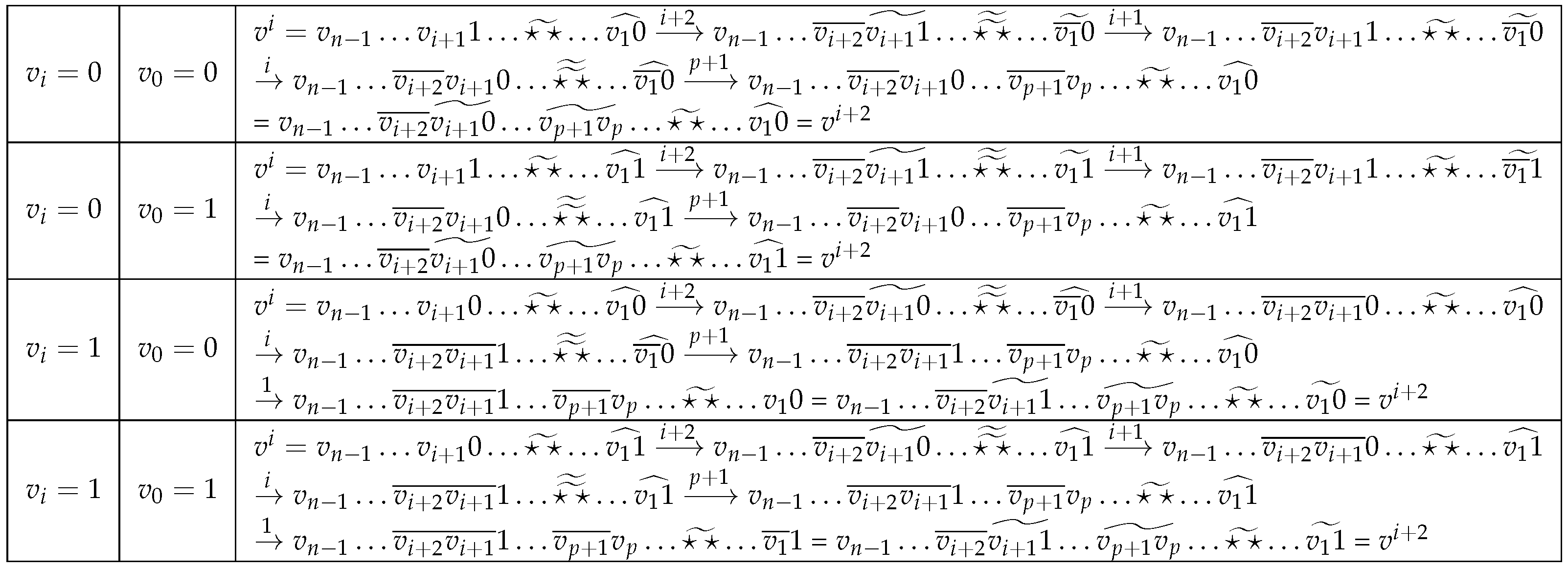
Figure 24 for ${\theta }_i=0$ (or Figure 25 for ${\theta }_i=1$) shows that ${\left({\left({\left({\left(v^i\right)}^{i+2}\right)}^{i+1}\right)}^i\right)}^{p+1}$ for all possible $v_i$ and $v_0$. Note that when ${\theta }_i=0$, ${\left({\left({\left(v^i\right)}^{i+2}\right)}^{i+1}\right)}^i$ can be found in Figure 16. Consequently, $\varphi \left({\left({\left({\left({\left(v^i\right)}^{i+2}\right)}^{i+1}\right)}^i\right)}^{p+1}\right)=\varphi \left(v^{i+2}\right)=u^{i+2}\ne {\left({\left({\left({\left(u^i\right)}^{i+2}\right)}^{i+1}\right)}^i\right)}^{p+1}$. □

Figure 24. The shortest paths from $v^i$ to $v^j$ when ${\theta }_i=0$.

Figure 25. The shortest paths from $v^i$ to $v^j$ when ${\theta }_i=1$.

Lemma 27. 

$Orb\left(TC{Q}_5\right)\ge 2$, $Orb\left(TC{Q}_6\right)\ge 2$, and $Orb\left(TC{Q}_n\right)\ge 2^{\lfloor {\displaystyle \frac{n-1}{2}}\rfloor }$ for $n\ge 7$.

Proof. 

As shown in Lemma 22, $Orb\left(TC{Q}_5\right)\ge 2$, and $Orb\left(TC{Q}_6\right)\ge 2$. Lemmas 22, 25, and 26 imply that $Orb\left(TC{Q}_n\right)\ge 2^{\lfloor {\displaystyle \frac{n-1}{2}}\rfloor }$ for $n\ge 7$. □

Theorem 1. 

$$Orb\left(FC{Q}_n\right)=\left\{\begin{array}{cc}1\hfill & ifn\le 4\hfill \\ 2\hfill & ifn=5,6\hfill \\ 2^{\lfloor {\displaystyle \frac{n-1}{2}}\rfloor }\hfill & ifn\ge 7.\hfill \end{array}\right.$$

Proof. 

According to Lemmas 1, 11, and 27, this theorem holds. □

3. Conclusions

Liu, Lan, Chou, and Chen [3] demonstrated that $Orb\left(LTC{Q}_n\right)=2$ for $n\ge 4$. Shiau, Wang, and Pai [5] proved that $Orb\left(C{Q}_n\right)=2^{\lceil {\displaystyle \frac{n}{2}}\rceil -2}$ for $n\ge 3$. Liu [7] established that $Orb\left(FC{Q}_n\right)=2^{\lceil {\displaystyle \frac{n}{2}}\rceil -1}$ for odd $n\ge 3$ and $Orb\left(FC{Q}_n\right)=2^{\lceil {\displaystyle \frac{n}{2}}\rceil -2}$ for even $n\ge 6$. In this paper, we show that $Orb\left(TC{Q}_n\right)=1$ if $n\le 4$, $Orb\left(TC{Q}_5\right)=Orb\left(TC{Q}_6\right)=2$ and $Orb\left(TC{Q}_n\right)=2^{\lfloor {\displaystyle \frac{n-1}{2}}\rfloor }$ if $n\ge 7$. Future research could focus on determining the orbit numbers of other hypercube-like interconnection networks, such as extended crossed cubes, extended folded cubes, and m$\ddot{o}$bius cubes.

References

- Efe, K. A variation on the hypercube with lower diameter. IEEE Trans. Comput. 1991, 40, 1312–1316. [Google Scholar] [CrossRef]
- Efe, K. The crossed cube architecture for parallel computation. IEEE Trans. Parallel Distrib. Syst. 1992, 3, 513–524. [Google Scholar] [CrossRef]
- Liu, Y.-J.; Lan, J.K.; Chou, W.Y.; Chen, C. Constructing independent spanning trees for locally twisted cubes. Theor. Comput. Sci. 2011, 412, 2237–2252. [Google Scholar] [CrossRef]
- Kulasinghe, P.; Bettayeb, S. Multiply-twisted hypercube with five or more dimensions is not vertex-transitive. Inf. Process. Lett. 1995, 53, 33–36. [Google Scholar] [CrossRef]
- Shiau, T.-H.; Wang, Y.-L.; Pai, K.-J. The orbits of Crossed Cubes. Available online: https://scirate.com/arxiv/1707.06763 (accessed on 24 July 2017).
- Frucht, R. Herstellung von Graphen mit vorgegebener abstrakter Gruppe. Compos. Math. 1939, 6, 239–250. [Google Scholar]
- Liu, J.J. The Orbits of Folded Crossed Cubes. Comput. J. 2024, 67, 1719–1726. [Google Scholar] [CrossRef]
- Wang, D.; Zhao, L. The twisted-cube connected networks. J. Comput. Sci. Technol. 1999, 2, 181–187. [Google Scholar] [CrossRef]
- Fan, J.; Lin, X.; Pan, Y.; Jia, X. Optimal fault-tolerent embedding of paths in twisted cubes. J. Parallel Distrib. Comput. 2007, 67, 205–214. [Google Scholar] [CrossRef]
- Fan, J.; Jia, X.; Lin, X. Embedding of cycles in twisted cubes with edge-pancyclic. Algorithmica 2008, 51, 264–282. [Google Scholar] [CrossRef]
- Lai, C.-J.; Tsai, C.-H. Embedding a family of meshes into twisted cubes. Inf. Process. Lett. 2008, 108, 326–330. [Google Scholar] [CrossRef]
- Lin, M.-S.; Chang, M.-S.; Chen, D.-J. Efficient algorithms for reliability analysis of distributed computing systems. Inf. Sci. 1999, 117, 89–106. [Google Scholar] [CrossRef]
- Li, X.; Lu, L.; Zhou, S. Conditional diagnosability of twisted cube connected networks, In Proceedings of International Conference on Computer Science and Information Technology. Advances in Intelligent Systems and Computing, Kunming, China, 27–28 December 2014; Springer: New Delhi, India, 2014. [Google Scholar]
- Wang, D.; Liu, Y. Almost Pancyclic Property of the Twisted-Cube Connected Network. Chin. J. Northeast. Univ. (Nat. Sci.) 1999, 20, 12–14. [Google Scholar]
- Wang, Y.; Zhou, J.F.G.; Jia, X. Independent spanning trees on twisted cubes. J. Parallel Distrib. Comput. 2012, 72, 58–69. [Google Scholar] [CrossRef]
- Guo, L. Reliability analysis of twisted cubes. Theor. Comput. Sci. 2018, 707, 96–101. [Google Scholar] [CrossRef]
- Wang, X.; Liang, J.; Qi, D.; Lin, W. The twisted crossed cube. Concurr. Comput. Pract. Exp. 2016, 28, 1507–1526. [Google Scholar] [CrossRef]
Disclaimer/Publisher’s Note: The statements, opinions and data contained in all publications are solely those of the individual author(s) and contributor(s) and not of MDPI and/or the editor(s). MDPI and/or the editor(s) disclaim responsibility for any injury to people or property resulting from any ideas, methods, instructions or products referred to in the content. |
© 2024 by the author. Licensee MDPI, Basel, Switzerland. This article is an open access article distributed under the terms and conditions of the Creative Commons Attribution (CC BY) license (https://creativecommons.org/licenses/by/4.0/).