Abstract
The structural gravimetry problem, which involves determining the geometry of a contact surface between two homogeneous layers based on observed gravity fields, is addressed in this paper. The method of local corrections is presented in a generalized form to improve its applicability to a broader range of problems. This study introduces several improvements to the local corrections method, including the use of a finite element approach for more accurate field calculations, particularly for near-surface boundaries. Additionally, the method incorporates prior knowledge of the boundary geometry, which serves as an initial approximation to enhance convergence and avoid potential divergence issues. Demonstrations on several synthetic examples are performed, which show the advantages of the generalized form of the method. For the territory of the Middle Urals, Russia, the refinement of two crustal boundaries is performed (the Moho boundary and middle crust boundary).
Keywords:
structural gravimetry; local corrections method; gravity inversion; density contrast; complex interpretation MSC:
86-08
1. Introduction
The gravimetric problem of a contact surface between two homogeneous layers was initially studied in 1930 by Numerov [1] and later explored by Tsuboi and Fushida [2], Zamorev [3], and others. This so-called “structural gravimetry problem” involves a forward case where the gravity field is calculated based on a known boundary geometry and layer densities. The inverse problem, on the other hand, aims to determine the surface geometry given the observed gravity field, boundary depth, and layer densities.
This problem can be considered as a permissible simplification of the density distribution restoration problem by a given gravitational field. Such a simplification made it possible to obtain an approximate solution without significant computational resources. However, the restoration of the position of structural boundaries itself also has practical applications. For example, it can be used to determine the position of the Moho surface, the thickness of the sedimentary cover, the boundary between granite and basalt layers, and other internal crustal boundaries identified by changes in density.
Early research focused on the two-dimensional formulation of the problem. A new stage in the study started in the 1970s when Strakhov formulated the problem as that of logarithmic potential [4] and Fedorova and Tsirulskii [5] proved the two-parameter ambiguity in terms of depth and density contrast for it. However, in three dimensions, the kernel is not logarithmic, and these results are not directly applicable. Therefore, in three-dimensional cases, the main approach to solving the inverse gravimetric structural problem is the use of iterative methods.
Various iterative methods can be used, including gradient methods [6] or inversion of the forward problem operator. The latter leads to a SLAE, which can be solved with algebraic methods. The complexity and the significant number of arithmetic operations, which are required for gradient calculations or matrix inversion are significant drawbacks of such methods.
One method with a different approach is the method of local corrections [7], which was specially developed for gravimetric problems. It requires a lower number of arithmetic operations and has the advantage of being designed for non-linear problem solving, although it does not require non-linear minimization. The method of local corrections has been applied in practical problems, both as an independent method [8,9] and as a technique for providing an initial approximation for further refinement using classical non-linear minimization methods [10]. In this paper we present a generalization of this method, making it more effective and applicable to a broader range of problems.
2. Methods
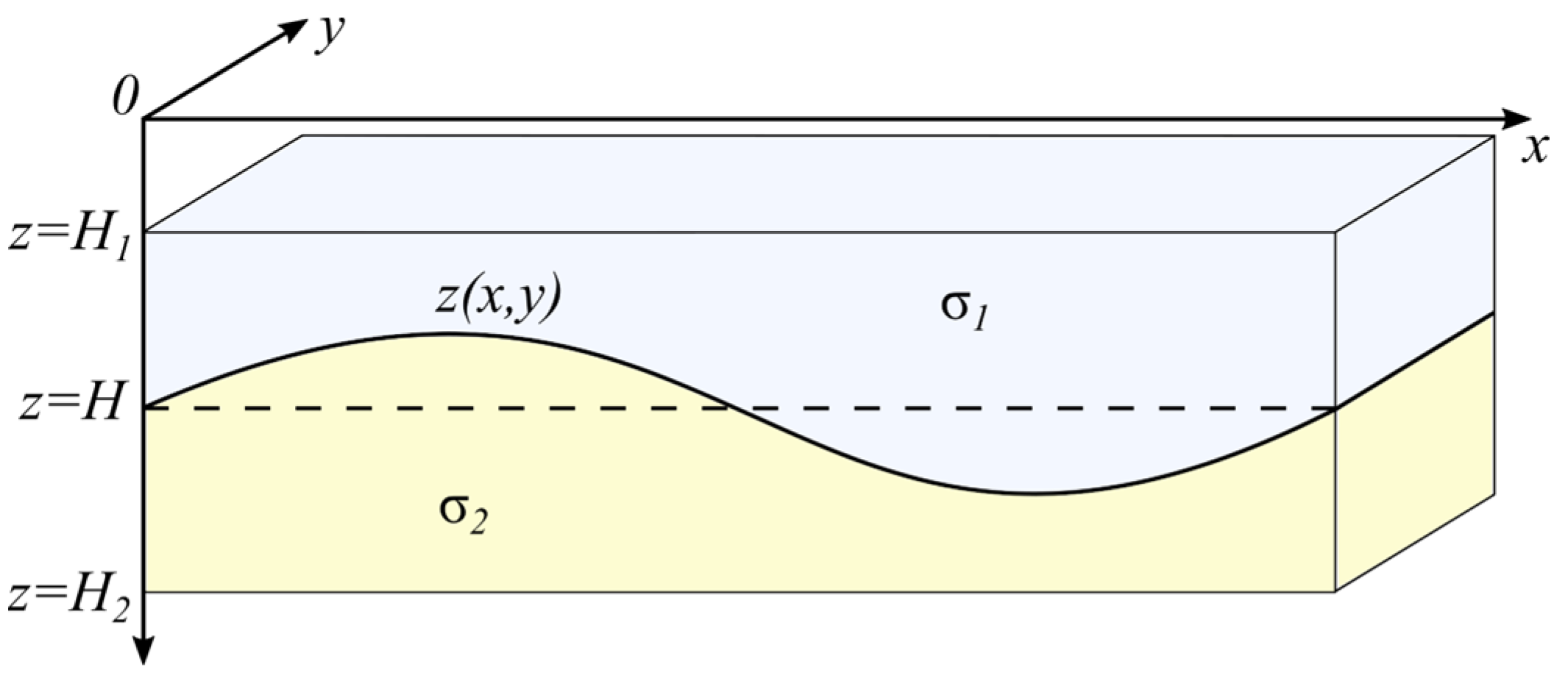
Let us define the structural gravity problem. Consider two layers (Figure 1). The upper layer is bounded by the plane at the top and by the surface at the bottom. The lower layer is bounded by at the top and by the plane at the bottom. The density of the upper layer density is , and the density of the lower layer is . The surface has a horizontal asymptotic plane .
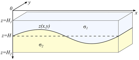
Figure 1.
The problem of the contact surface in a three-dimensional form.
In this case, the anomalous gravity field is produced by the depth inhomogeneity of the model. This is, in turn, due to the non-flat nature of , so we will refer to it as the gravitational field of the boundary . The field value, observed at the point , can be calculated using the following Equation (7):
where is the difference between densities below and above the boundary (the density contrast), and —the gravity constant.
The original formula for the local corrections method for structural boundaries was given in [7]. That form of the formula is for unit density, and the gravity constant is omitted, as follows:
where is the observed field, and is the field of , the -th iteration of the boundary. Both and are given in a discretized form. It is assumed that they are given on a grid and that the indices and define the position of a grid element. Indices i and j are the same for the field and boundary grids, and this reflects the main idea of the local corrections method, which is to reduce the field error at some point on the Earth’s surface by changing the boundary right below the observation point only. The values of the fields for the successive approximations are calculated using Formula (1). To avoid a situation where the method diverges, Prutkin also suggested using the idea of Tikhonov’s regularization. Instead of in Equation (2), should be used. Taking all this into account, the ready-to-use formula for the original local corrections method is as follows [11]:
where is the value which is selected by the researcher, and is the cubature formula coefficient (i.e., the square of a discretization element). The original parameter is the combination of constants: . Usually, the coefficient is selected to be relatively small (). Its purpose is to initiate the selection in the desired direction and to reduce the boundary change between iterations. The latter results in an increased number of iterations, which are required to achieve the desired accuracy, so it is important to choose an appropriate value for the parameter. Note that such usage is not actually the regularization in the Tikhonov sense. This coefficient is required to reduce the field difference amplitude, thus preventing the abrupt change in between iterations. It is, therefore, better to refer to as a coefficient for stabilization rather than regularization.
There are several improvements which could be made to the local corrections method to make it applicable to a broader range of cases. Let us refer to the resulting algorithm as the generalized local corrections method (GLCM) for the structural gravity problem.
The first improvement is needed to avoid weak singularity at (, and ) in Formula (1). One solution is to shift the grid of field calculation relative to the boundary grid . However, this method introduces an additional error (especially for sparse grids). We will use an alternative approach to calculate the field. Instead of directly computing the integral Equation (1), we will adopt the finite element approach [11].
We will divide the volume located between the boundary and its asymptote into a set of elementary shapes, whose gravitational effect can be calculated analytically. This transition moves us from the model of an infinite layer to a model in which the gravitational field is generated by a finite, bounded body, which, nonetheless, corresponds to practical applications.
Let us define a partition of the integration variables on a rectangular grid defined by , and construct elementary prisms with unit density and height with grid cells as bases (Figure 2). The field of the layer bounded by the surface and flat plane is equal to the sum of the fields from all the partition elements.
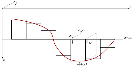
Figure 2.
Discretization of the volume between the boundary and its asymptote (vertical cut).
For the rectangular prism the gravity effect can be calculated directly using the following formula [12]:
where . As in Equation (1), the is the point at the Earth’s surface where the field is being calculated. When the coordinates of the prism are substituted for all 3 axes, the complete formula includes 8 calculations of arctangent function, 16 logarithm function calculations, and 8 square root calculations (for ). In contrast, numerical integration for Equation (1) using, for example, the midpoint rule, would require only 2 square root operations per discretization element. Thus, calculations using the FEM approach, despite being free from weak singularities, require more computation resources. Also, if a more accurate method than the midpoint rule is used for the integral calculation, its accuracy will surpass that of rectangular prism approach.
Now we derive a separate formula for the local correction method in the case of near-surface boundaries. We will apply the idea of local corrections method to Equation (5). Consider that the field at point is produced by one prism located directly under only. The field calculation point is located above the prism center, as follows:
Using this in Equation (5) and taking into account that Equation (5) itself is the vertical derivative of gravity potential, which for the prism is equal to , and since the vertical line, which crosses , is the axis of symmetry for the prism, a simplified equation is obtained, as follows:
where . With and , we denote the grid step length along the and axes correspondingly: , .
According to local corrections method idea, at each iteration the field value in a point is changed proportionally to the change in the boundary depth, as follows:
Using Equation (7), we obtain the generalized formula for the generalized local corrections method, as follows:
where , which is defined by the selected discretization. The closer is to the field calculation plane, the bigger the grid step could be. If , then Formula (9) can be reduced to the following form:
This is analogue for Equation (2). On the contrary, for shallow boundaries (), Equation (9) can be reduced to the following form:
The same stabilization coefficient as in Equation (3) can be applied to the right-hand sides of Equations (10) and (11) to reduce the amplitude of the field difference: . However, in practice, there is usually no need to perform such a stabilization of the iterative process when using Equation (11). The physical meaning of Equation (11) is obvious from the fact that the field of an infinite layer with thickness H is equal to . The unstable nature of Equation (10) is due to the fact that the depth values are in the denominators. We need to limit the increment of artificially to prevent the depth from approaching zero. Although the formula is intended for deep boundaries, during the iteration process, there might be situations where the boundary approaches the surface. On the other hand, for deep boundaries, a large change in amplitude causes a relatively small field change (and vice versa), and this may result in geologically impossible high-amplitude boundaries. To prevent such effects, the parameter is introduced. In Formula (11), the relationship between the change in depth and the change in the field is linear, so such stabilization is not required.
An important consequence of the transition to solving the direct structural problem of gravimetry using the finite element method is the weakening of the requirements imposed on a boundary. In the integral Equation (1), it is assumed that the boundary has an infinite length and reaches the asymptote . Obviously, when solving practical problems for real planets, the requirement of infinite length is always not met. However, due to the condition of the existence of the asymptote, it is expected that at the boundary of the area under study, the amplitude of the surface is significantly lower than in the central part of the area. Such a boundary configuration makes it possible to reduce the “edge effect”—an abrupt decrease in the field amplitude when the counting point goes beyond the boundaries of the area under study. When using the finite element approach, the concept of an asymptote becomes inapplicable. Any horizontal plane can serve as an “asymptote”, while density contrast above such an “asymptote” is positive, while it negative when it is below. A change in the position of the “asymptote” entails a change in the values of the calculated field by a constant; therefore, when using the generalized method of local corrections, the value of the “asymptote” depth is fixed and does not change between iterations. When solving the direct problem, it is convenient to choose the average value of the boundary location as the depth of such an “asymptote”: .
When solving practical problems, a significant contribution to the resulting solution is made by the person—the interpreter. Based on their experience and views, the interpreters selects from a variety of possible solutions to ill-posed problems those that they personally think are more correct. It is possible to reduce such bias in the study by using additional objective data obtained by other geophysical methods. In the case of the local correction method for a structural gravimetry problem, such additional objective information can be a previously known boundary geometry obtained from seismometric studies. This geometry is provided to the algorithm as the initial position of the boundary . Thus, when solving a direct problem, the process begins not from the flat boundary of the zero approximation, but from the boundary that already contains a priori information about the nature of the desired surface.
In summary, the generalized method of local corrections for solving the structural inverse problem of gravimetry has the following distinctions from the method in its original formulation:
- It uses the boundary of the zero approximation (constructed based on a priori data) instead of a flat asymptote, which allows for the initiation of the fitting process in the desired direction, thereby increasing the convergence speed.
- A finite element scheme is employed for the direct problem calculation stage, making the method applicable to boundaries that reach the surface.
- For near-surface boundaries, a special more stable Formula (11) is used.
The following pseudocode (Algorithm 1) presents all steps of the algorithm for gravity inversion using GLCM.
| Algorithm 1. Numerical solution to forward and inverse structural density problems |
| Input: U[0…N, 0...M]—observed gravity field Z[0...N, 0...M]—initial approximation for the boundary StepX, StepY—grid step in x and y directions for U and Z LeftX, BottomY—grid bottom left corner coordinates for U and Z —stabilization coefficient —density contrast —gravity constant Field calculation using FEM: function CalcField(boundary, depth): result = [,] for n = 0 to N: for m = 0 to M: // Field calculation point x’, y’ = GetGeoCoordinates(n,m) value = 0 for i = 0 to N: for j = 0 to M: //Center of prism projection rectangle x,y = GetGeoCoordinates(i,j) value += Vz3(x’, y’, x—StepX/2, x + StepX/2, y—StepY/2, y + StepY/2, depth, boundary[i,j]) result[i,j] = γ × ∆σ × value // Convert indexes to coordinates function GetGeoCoordinates(i,j): return LeftX + i × StepX, BottomY + j × StepY // x,y—observation point, remaining parameters define prism position function Vz3(x, y, x1, x2, y1, y2, z1, z2): return Vz2(x, y, x2, y1, y2, z1, z2)−Vz2(x, y, x1, y1, y2, z1, z2) function Vz2(x, y, ξ, y1, y2, z1, z2): return Vz1(x, y, ξ, y2, z1, z2)−Vz1(x, y, ξ, y1, z1, z2) function Vz1(x, y, ξ, η, z1, z2): return Vz(x, y, ξ, η, z2)−Vz(x, y, ξ, η, z1) function Vz(x, y, ξ, η, ζ): ∆x = ξ−x ∆y = η−y R = Sqrt(∆x × ∆x + ∆y × ∆y + ζ × ζ) return (η == y ? 0 : ∆y × Log(Abs(∆x) + R)) + (ξ == x ? 0 : ∆x × Log(Abs(∆y) + R)) - ζ × Arctan(∆x × ∆y / (ζ × R)) Inversion with GLCM: / (StepX × StepX × γ × ∆σ) // Z is updated on each iteration, but H should be constant H = Avg(Z) for i = 0 to MaxIterationsCount: Un = CalcField(Z, H) for n = 0 to N: for m = 0 to M: // In case of deep boundary Z[n,m] = Z[n,m] / (1 + × (U[n,m]−Un[n,m])) is optional) Z[n,m] = Z[n,m] + × (U[n,m]−Un[n,m])/2πγΔσ Output: Z[0…N, 0…M]—the restored boundary |
We will test the methodology described above on a series of synthetic examples and then apply it to a real case of recovering the position of the interface between two media in the Earth’s crust. The construction and calculation of the model examples are detailed in the corresponding section of the article. For the practical example, we will use the observed gravitational field for the Urals territory. However, the observed field contains information from the entire thickness of the crust, while we need components specifically related to the depths of the boundaries to be recovered. To obtain these components, we use a depth source separation method [13], based on transformations of the field with a recalculation technique. As a result, we obtain a set of uniformly distributed fields corresponding to horizontal layers of the Earth’s crust. For each boundary to be recovered, a set of such fields is selected for its depth interval […], and the fields are summed. The resulting sum is considered the field of the recovered boundary.
The initial approximation of the boundary can come from various sources. We will use the Crust 1.0 model [14] in one case. This model has a resolution of 1° × 1° and, thus, is well-suited for the initial approximation for the boundaries, which are included in it.
For another case, we have selected a different source for the initial boundary. The 3D density model of the Urals region, which has been constructed by transformation and interpolation of initial seismic (DSS) data, was utilized [15] (p. 171). Using a previously developed algorithm for density isosurface selection [16], an isosurface is extracted from the density model for a specific density value. This surface is used as the initial approximation for the generalized method of local corrections. This method is able to provide more detailed surfaces than the ones taken from the Crust 1.0 model.
3. Model Examples
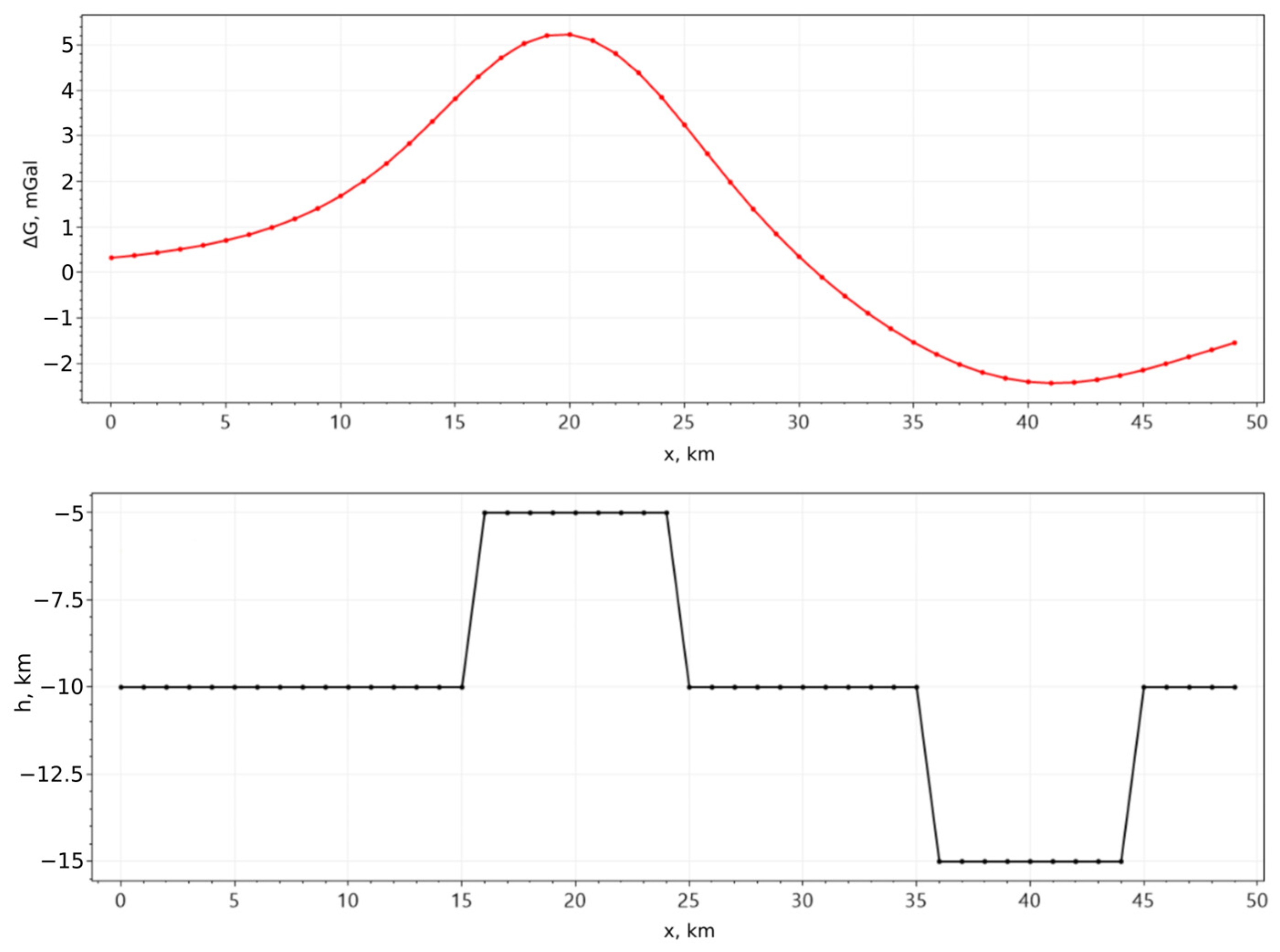
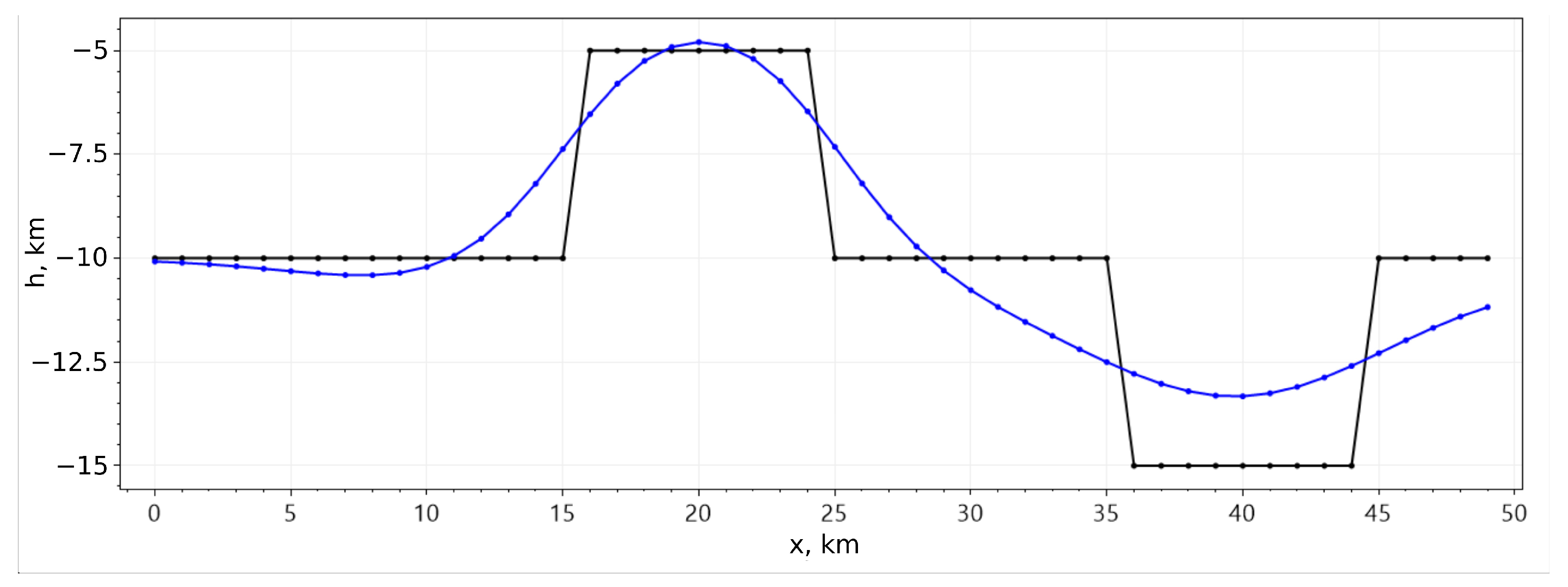
Let us consider a model example. Suppose there are two local objects (a protrusion and a depression) located at a depth below the Earth’s surface, symmetrically positioned relative to a plane at a depth of km (Figure 3, lower). The model has the following parameters: a resolution of 50 × 50 points and a grid spacing of 1 km in both directions. The density of the upper layer is 2.3 g/cm3, and the density of the lower layer is 2.4 g/cm3, and, therefore, g/cm3. The recovery was conducted using a flat plane km as the initial approximation. It took 19 iterations (with to achieve a root mean square (RMS) deviation of RMS < 1 for the recovered boundary from the initial one. The result of the recovery is shown in Figure 4 (blue curve).

Figure 3.
Model example 1: boundary position (lower) and its gravity field (upper).
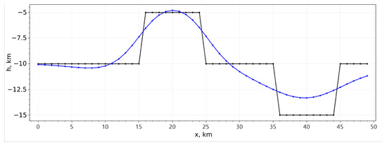
Figure 4.
Model example 1: original (black line) and reconstructed (blue line) boundaries.
As can be seen, the recoveries of the boundary when it is submerged below the asymptotic level are less accurate using this method than those when it is raised above the asymptote. This can be explained by the greater distance of the submergences from the Earth’s surface (where the field is calculated) and, accordingly, by the wider anomaly generated by the local depression of the boundary. Another factor contributing to the method’s lower sensitivity to submersions compared to uplifts is its reliance on the concept of locality. The method assumes that the primary contribution to the field comes from the boundary point located directly beneath the observation point. However, depending on the depth and geometry of the depression, a situation may arise where, in reality, the nearest (in terms of geometric distance) boundary point is not located directly beneath the observation point but instead lies under one of the neighboring field calculation points. In this case, the local corrections method underestimates the depth of the reconstructed boundary. To reduce the influence of this factor, it is essential to select the most suitable initial approximation of the boundary.
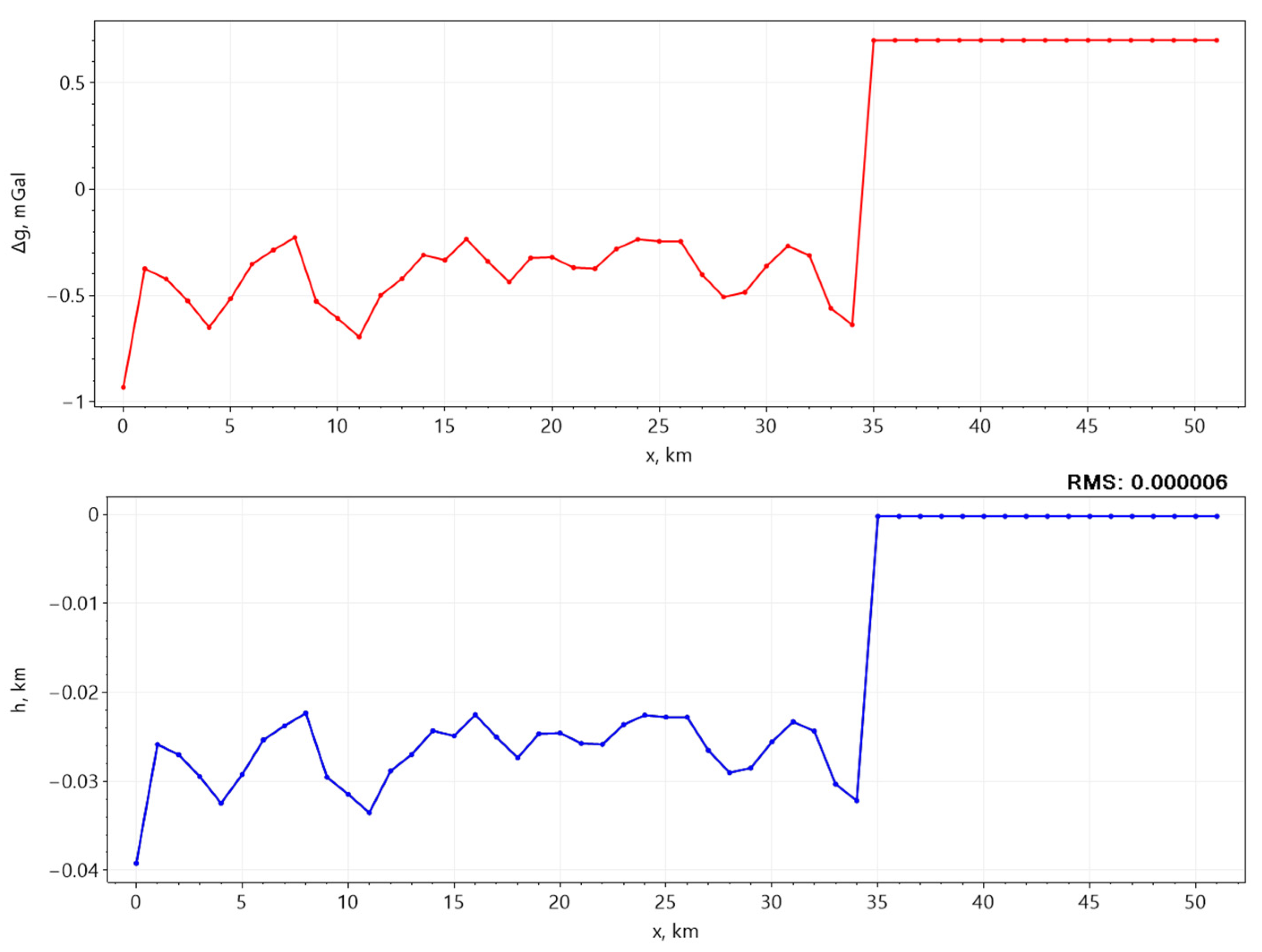
Consider a case where the “classical” version of the local corrections method is not applicable. In the lower part of Figure 5, a cross-section of the structural boundary extending to the Earth’s surface is shown. When the field calculation is performed on the same grid where the boundary is defined, Equation (1) cannot be applied. However, using Equations (4) and (5), this becomes feasible. The use of the formula for near-surface anomalies (11) allows us to obtain a solution already in the first iteration, which visually matches the original boundary exactly in appearance (lower part of Figure 5). The root mean square deviation of the recovered boundary from the original is of an order of . Such rapid convergence without any stabilization is explained by the relationship between the grid spacing (about 20 km) and the boundary depth (about 20 m). In this case, the dominant contribution to the gravitational field comes from the point directly beneath the measurement point, and the contributions from the others can be neglected. This is also reflected in the full morphological similarity between the boundary and its field.
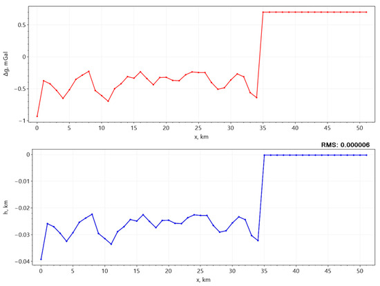
Figure 5.
Model example 2. Boundary that meets the Earth’s surface level (below) and its gravity field (upper).
The following model example illustrates the application of the method to “jagged” boundaries (Figure 6). The model is based on model example 1, but uniform noise with an amplitude equal to 5% of the boundary’s amplitude is added to the boundary. Although the noise is not visually evident in the gravitational field, reconstructing the boundary became difficult. Using the same reconstruction parameters (the initial approximation is that the asymptote is at km, ), 27 iterations were required to achieve an RMS < 1 value for the standard deviation between the original and reconstructed boundaries. Increasing the percentage of noise in the boundary causes a further increase in the number of iterations, as follows:
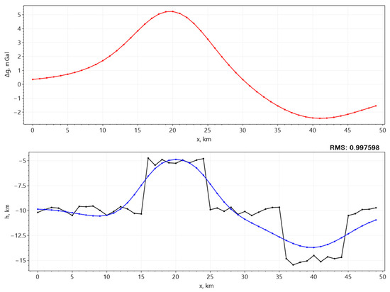
Figure 6.
Model example 3: a boundary complicated by random geometric variations (black line), its gravitational field (red line), and the position of the reconstructed boundary (blue line).
- For noise with an amplitude of 10% of the boundary amplitude, while maintaining other model parameters, achieving RMS < 1 required 88 iterations,
- For noise with an amplitude of 15% of the boundary amplitude, after 1000 iterations, the standard deviation of the boundaries difference was 1.127; the desired RMS < 1 could not be achieved.
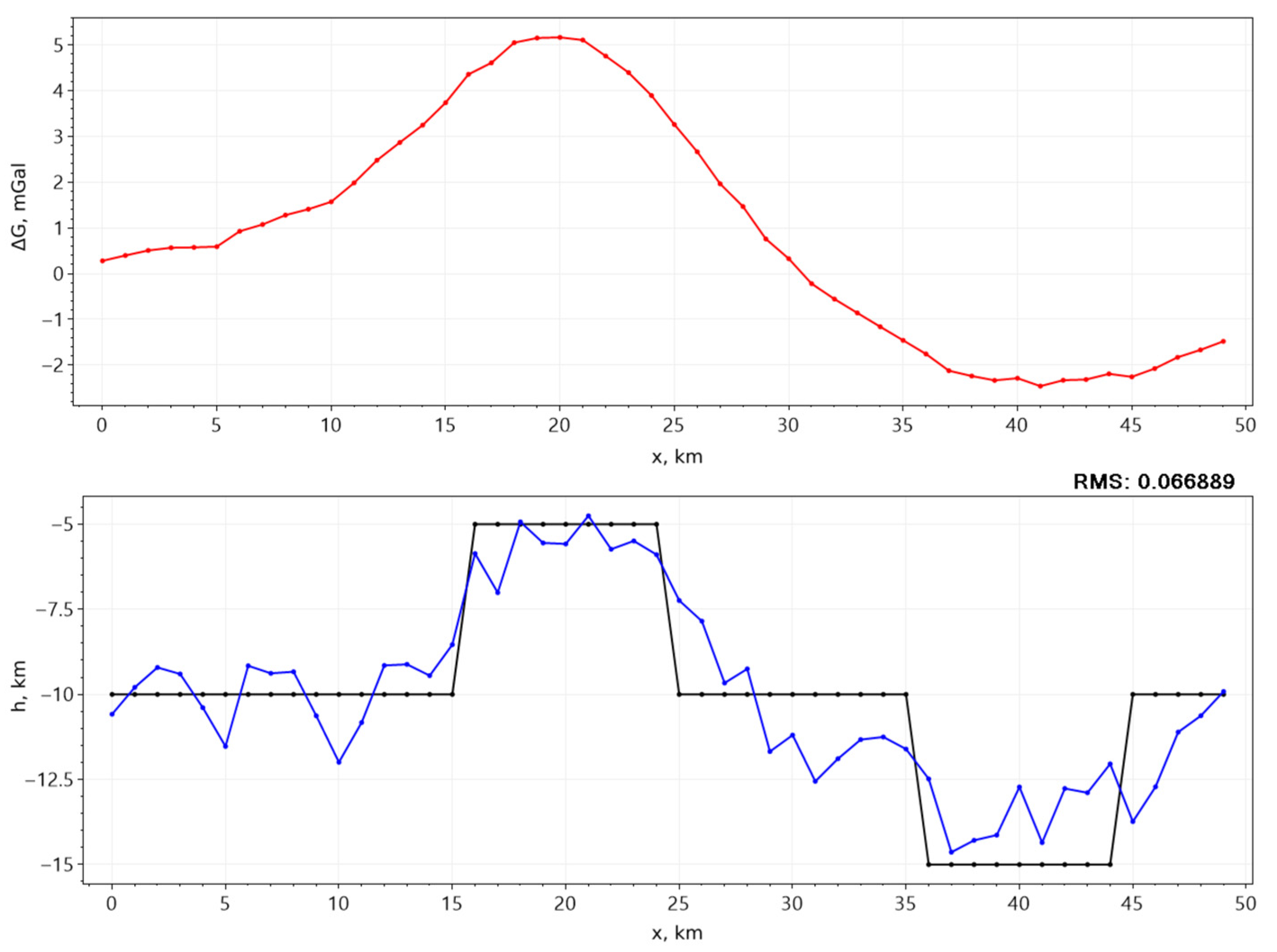
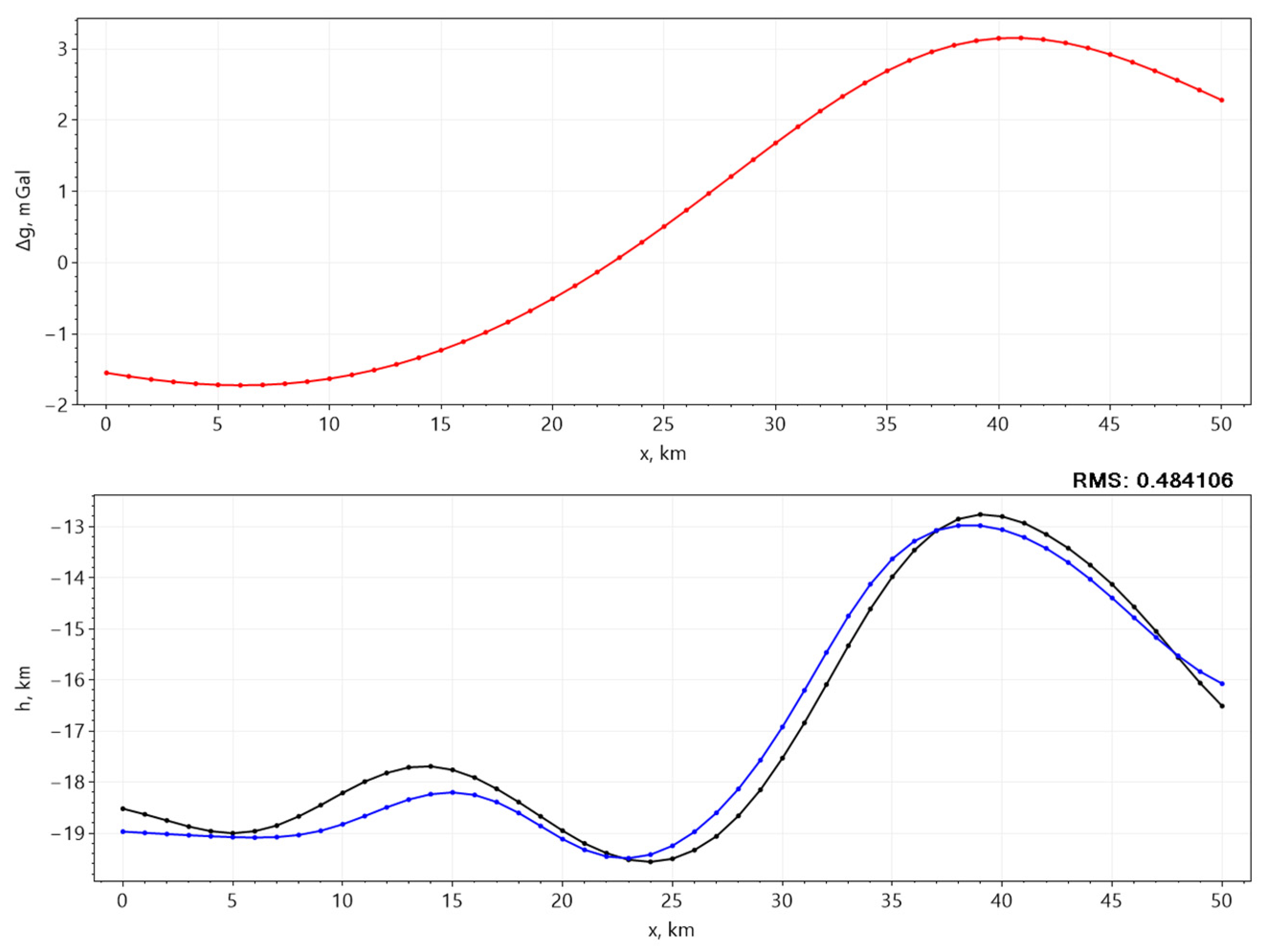
Model example 4 demonstrates the reconstruction of the boundary based on a field that is measured with measurement error. For this, the boundary from model example 1 is used, and uniform noise with an amplitude equal to 3% of the field’s amplitude is added to its gravitational field (Figure 7, top). After 50 solution iterations, the standard deviation between the reconstructed and original boundary is 0.067 (Figure 7, bottom).
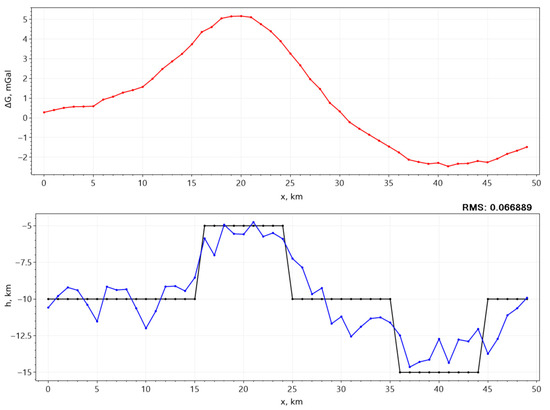
Figure 7.
Model example 4: a boundary similar to the boundary in example 1 (black line), with 3% noise added to its gravitational field (red line). The position of the reconstructed boundary is shown in blue.
Now we will conduct a similar experiment, but as an initial approximation boundary we will use a non-flat boundary instead of an asymptote. The original boundary position was taken as the initial approximation. Obviously, if the field had not been modified, such an iterative process would have converged in the first iteration. However, the introduced “measurement error” triggers the complete functioning of the algorithm. After 50 iterations, the standard deviation of the reconstructed boundary from the initial one was 0.065 (Figure 8), showing a slight decrease compared to the reconstruction using the asymptote.
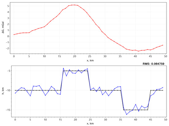
Figure 8.
A variation of model example 4 using the original boundary (black line) as the initial approximation in the first iteration. “Noised” gravitational field is shown in red, the result of restoration is the blue line.
Model example 5 shows how choosing the initial boundary approximation affects the convergence accuracy of the method. Consider a “quasi-real” boundary model (Figure 9a).

Figure 9.
Model example 5: a boundary with morphology similar to real boundaries of the Earth’s crust: (a) boundary position and (b) reconstruction result with a flat boundary.
We will conduct several sequential experiments on the calculated field to reconstruct the boundary position. The reconstruction parameters remain consistent across experiments: the depth of the “asymptote” is H km, , g/cm3, and the number of iterations is 50.
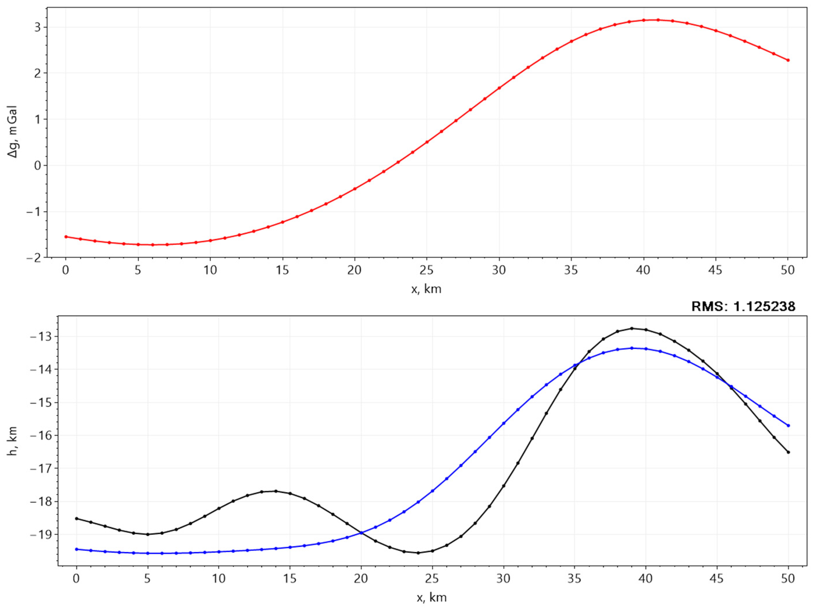
The first experiment is the reconstruction from a flat “asymptote”. Figure 9b shows a three-dimensional image of the obtained boundary, and Figure 10 presents a section (plane y = 25) of the observed field (red), the actual position of the boundary (black), and the reconstructed boundary (blue). The root mean square deviation of the reconstructed boundary from the original was 1.13. In the three-dimensional model of the reconstructed boundary, it is visually noticeable that only large-scale anomalies were reconstructed.
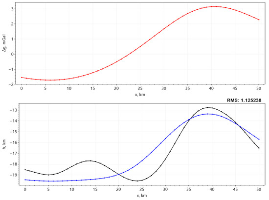
Figure 10.
Model example 5: reconstruction result with a flat boundary. Slice of the field (red line, top) and boundaries (bottom). The real boundary position is shown with the black line, the result of restoration is the blue line.
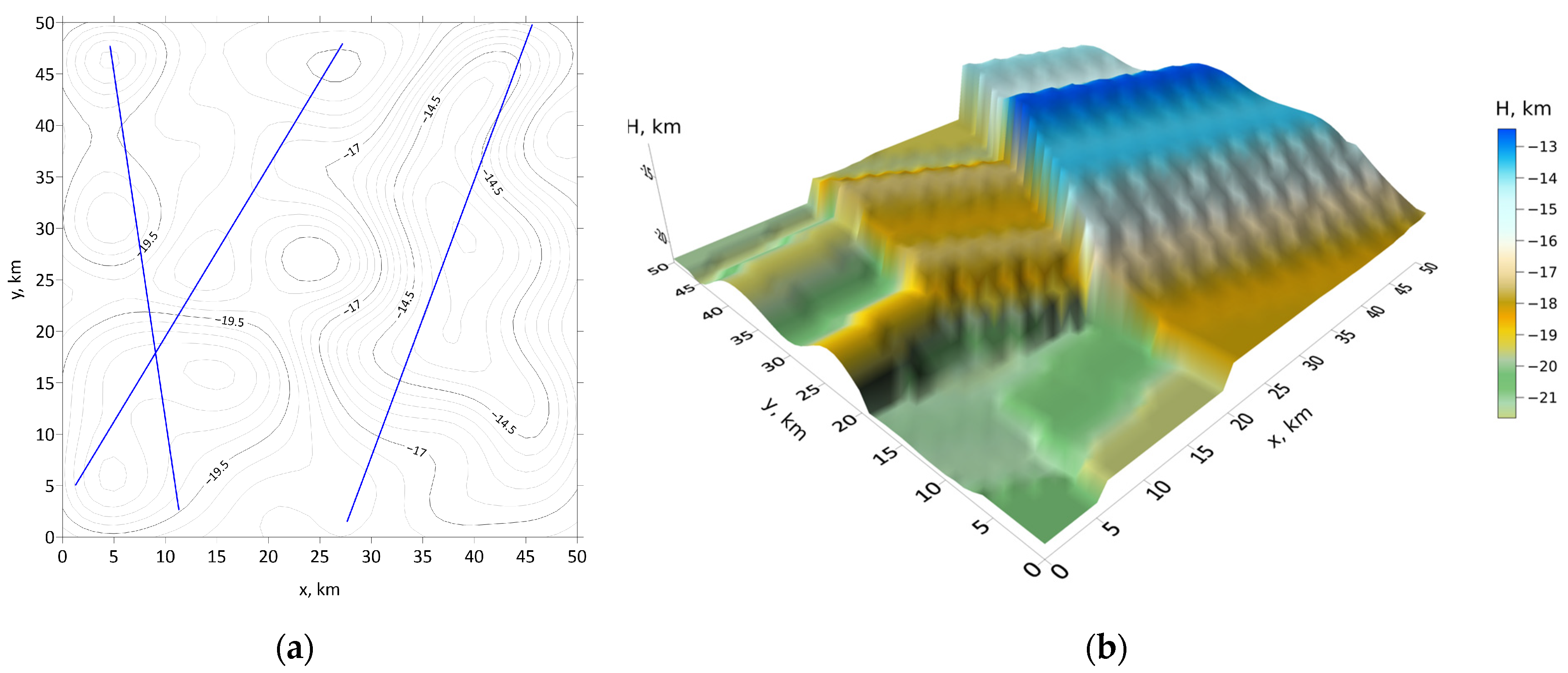
In the second experiment, we create an initial approximation surface, thereby simulating the use of a priori data on the surface geometry during the reconstruction process. Consider three profiles (Figure 11a), along which the depth data of the boundary is collected. In reality, this can be achieved using seismometric methods. The experiment uses the exact values of the depth of the actual boundary. These values are interpolated across the study area using the nearest neighbor method (Figure 11b).
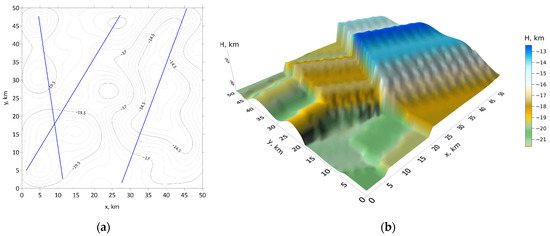
Figure 11.
Model example 5: three profiles case: (a) position of the profiles and (b) boundary of initial approximation, obtained using interpolated data.
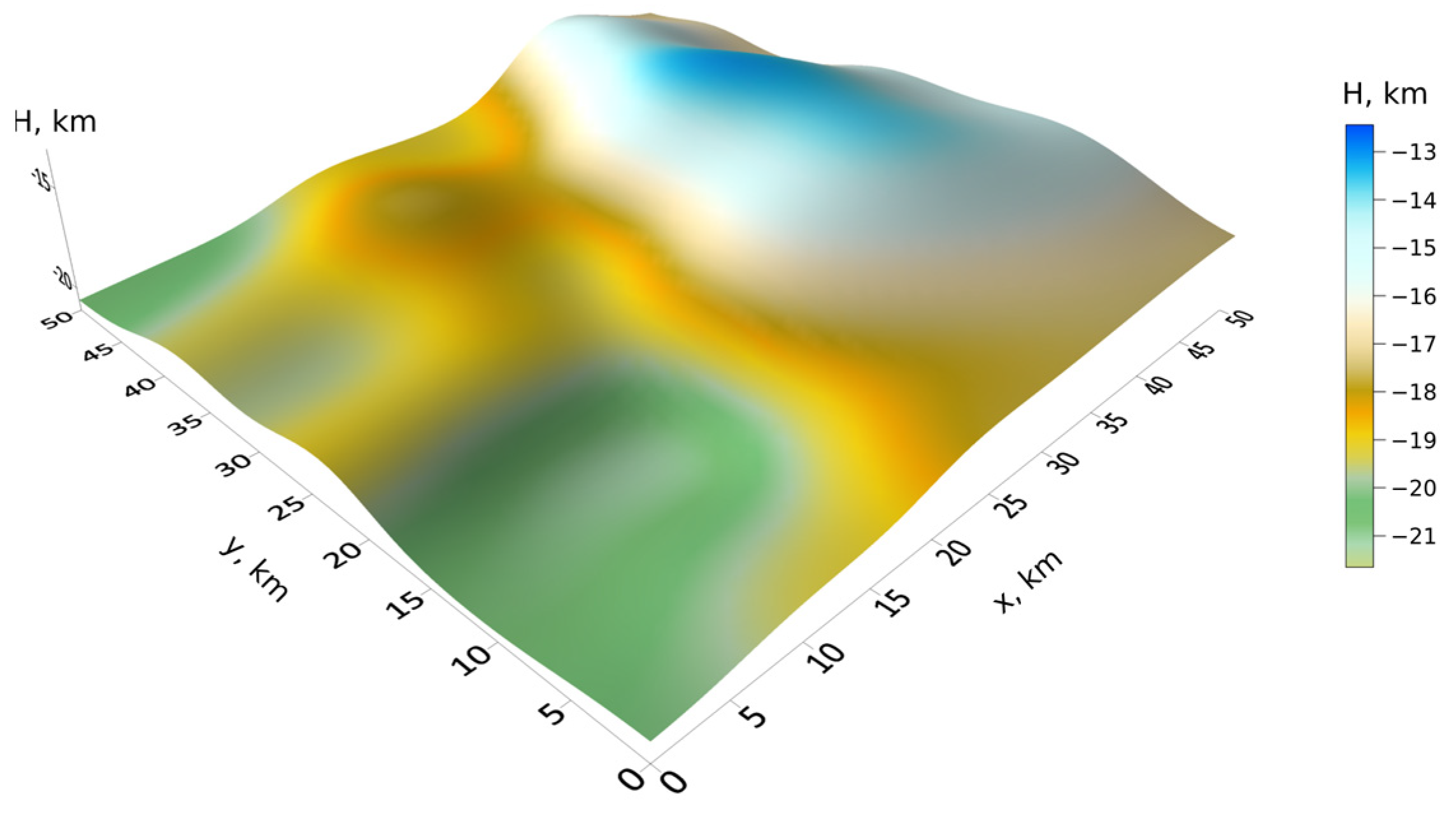
Now we use the interpolated boundary as the initial approximation in the local correction method. Figure 12 shows the result obtained after 50 iterations, and slices of the boundary and the field are shown in Figure 13. The standard deviation of the reconstructed boundary from the original one dropped to 0.61 (a 46% decrease compared to the first experiment).

Figure 12.
Model example 5: resulting boundary, obtained in the case of three profiles.
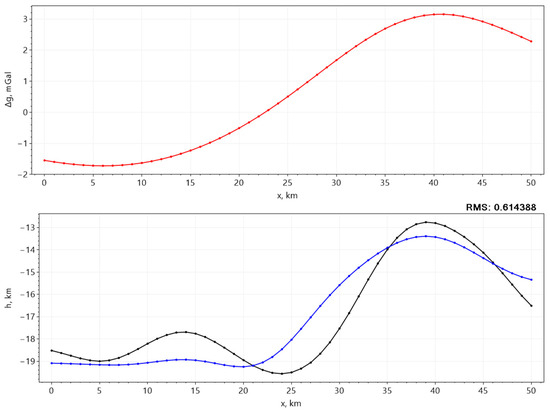
Figure 13.
Model example 5: reconstruction result with boundary, constructed using three profiles: slice of the field (red line, top) and boundaries (bottom). The real boundary position is shown with the black line, the result of restoration is the blue line.
The visually reconstructed surface in Figure 12, although showing significantly more details than the surface in Figure 9b, has an immersion in the center of the area with insufficient depth. This is due to the method’s lower sensitivity to immersions compared to uplifts, as demonstrated in model example 1. However, the use of a priori information allows us to reduce the influence of this factor. To illustrate this, we will conduct a third experiment. A fourth profile will be added to the model, specially positioned to capture the specified immersion, and the interpolation procedure will be repeated (Figure 14).
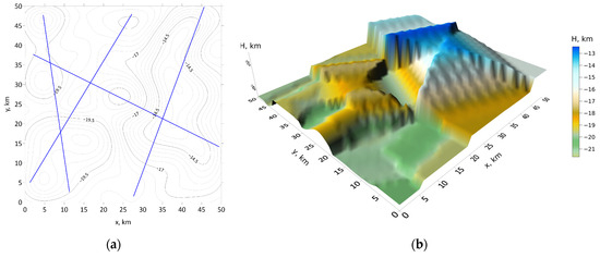
Figure 14.
Model example 5: four profiles case: (a) position of the profiles and (b) boundary of initial approximation, obtained using interpolated data.
We use the new position of the initial boundary in the local correction method restoration procedure. After 50 iterations, the RMS deviation of the restored boundary from the initial one was 0.48 (Figure 15 and Figure 16). This presents an additional 21% reduction in the discrepancy compared to the previous experiment.
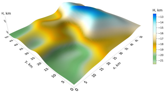
Figure 15.
Model example 5: resulting boundary, obtained in case of four profiles.

Figure 16.
Model example 5: reconstruction result with boundary, constructed using four profiles: slice of the field (red line, top) and boundaries (bottom). The real boundary position is shown with the black line, the result of restoration is the blue line.
This model example demonstrated that incorporating a priori data on the geometry of the reconstructed boundary as an initial approximation in the local correction method for structural boundaries can both increase the rate of convergence of the method and improve the accuracy of reconstruction.
4. Case Study
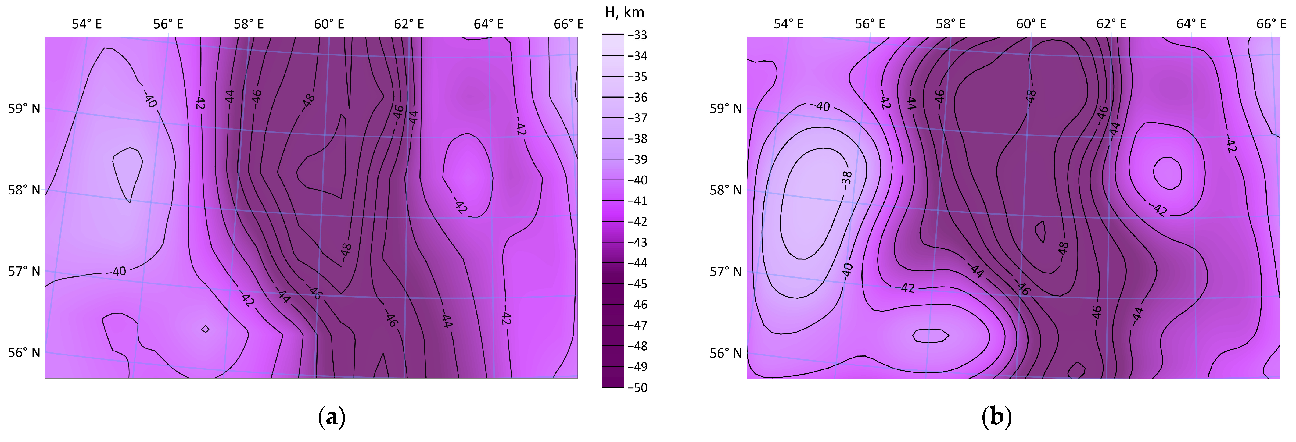
Now we will demonstrate the methodology using the example of reconstructing the position of the real boundaries of the Earth’s crust. The research area is located in the Middle Urals region (Russia). We will be reconstructing two crustal boundaries, the first being the Mohorovičić discontinuity (Moho), and the second being the boundary of the middle crust, determined by isolines of a density of 2.88 g/cm3.
To apply the method of local corrections, we will need an initial approximation of the boundary, the density contrast, and the gravity field. As for the last factor, we will take the component extracted from the observed field, which we will associate with sources located at the depth of the boundary being reconstructed. According to the results of previous studies [15], the observed field has already been uniformly divided into components of varying depths with a step of 1 km. This set of fields serves as the initial dataset.
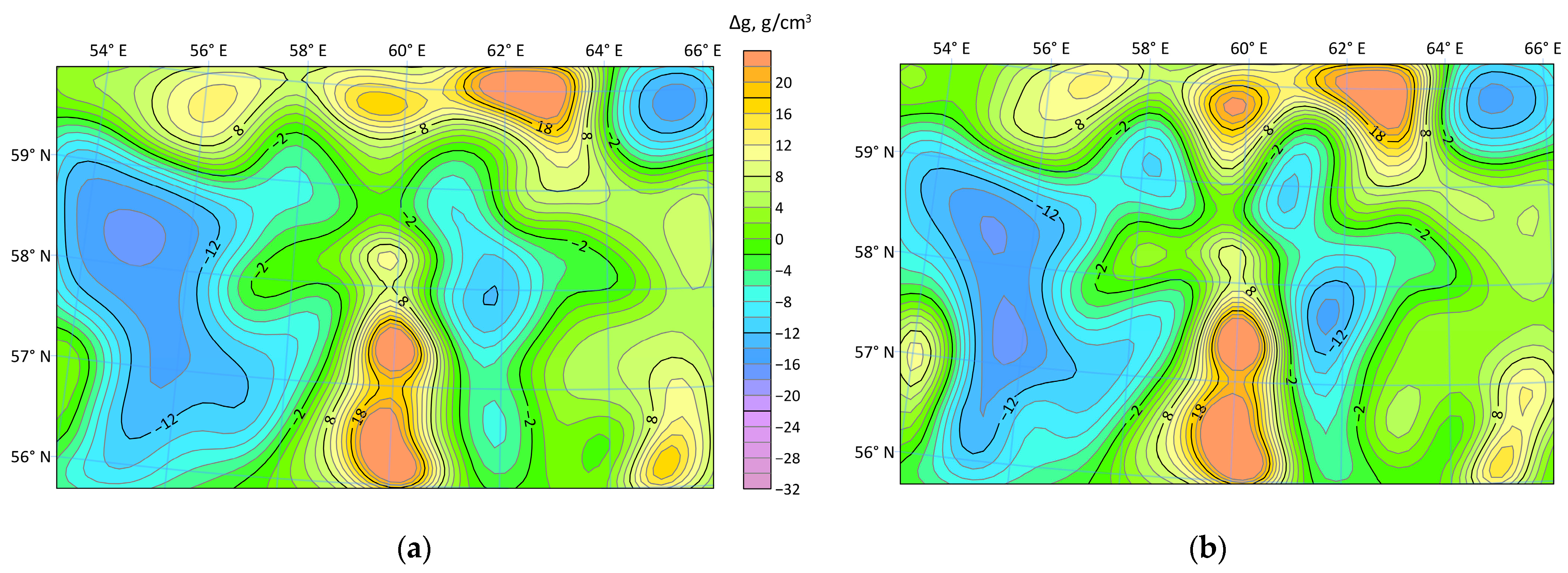
The initial approximation of the Moho boundary is based on the Crust 1.0 dataset (Figure 17a). Within the study area, the depths of this boundary range from 38.6 to 49.3 km. Based on the previously constructed density model of the initial approximation, the density contrast at the boundary is determined to be 0.2 g/cm3. This density is used to calculate the Moho boundary field.

Figure 17.
Moho boundary: (a) initial position; (b) refined with GLCM.
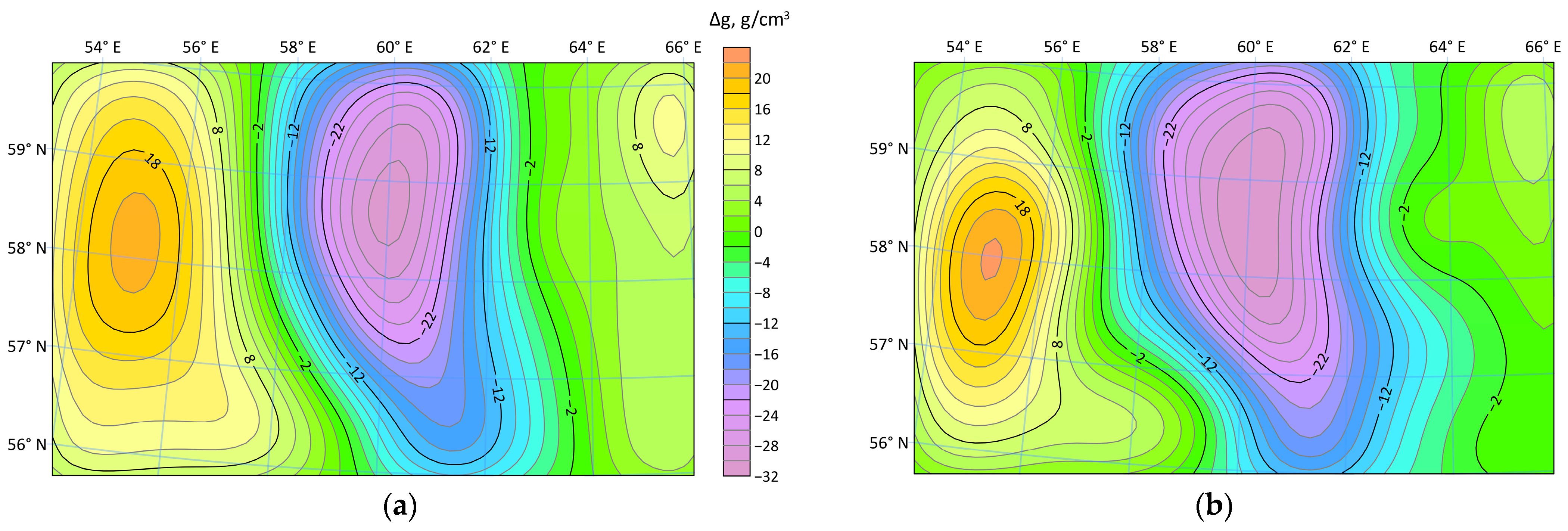
Next, considering the depth step of the separated source fields, we sum the components of the field corresponding to depths from 39 to 49 km. This summed field is then added to the field of the initial approximation boundary (Figure 18a). The resulting field is used as the observed input for the algorithm (Figure 18b).
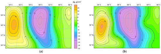
Figure 18.
Moho gravity fields: (a) for the initial boundary position; (b) corrected with the anomaly field of the masses located in the range of (−39, −49) km.
The next step is the boundary position refinement using GLCM. Equation (10) was used with , and 17 iterations were required to achieve RMS < 1 between the fields. Figure 17b presents the resulting boundary.
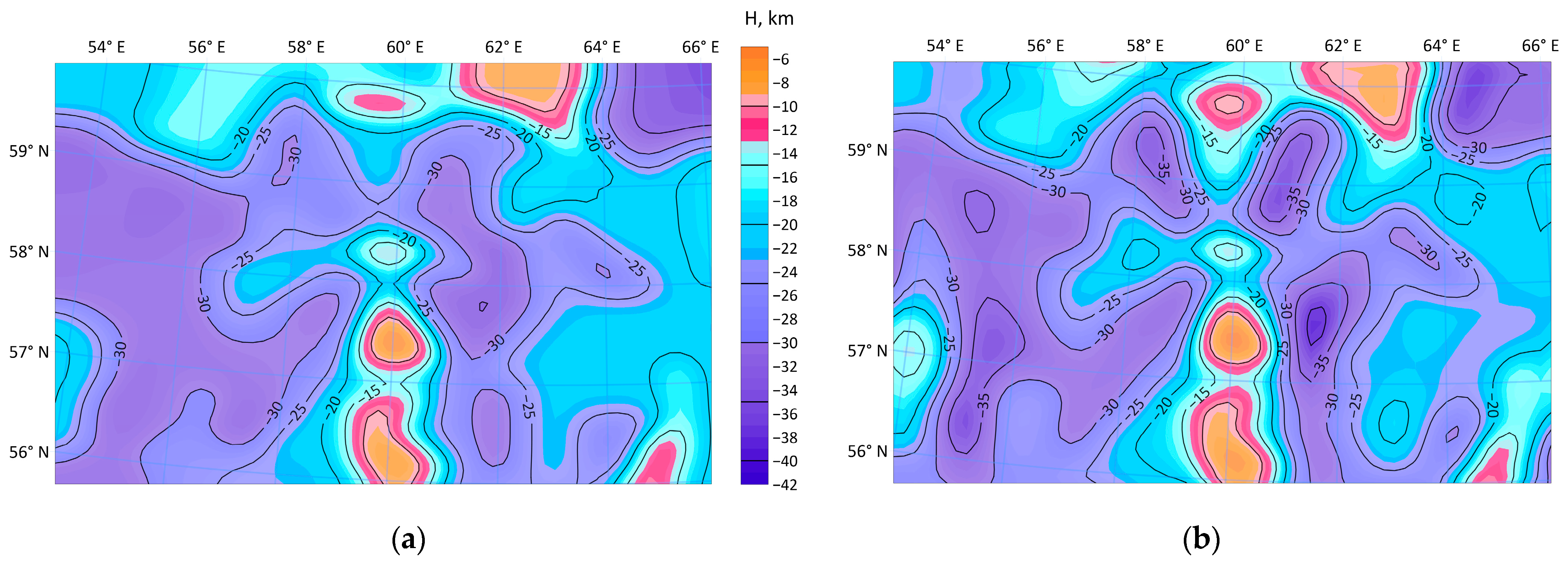
For the restoration of the middle crustal boundary, corresponding to a density value of 2.88 g/cm3, the same set of separated fields was used as for the Moho restoration. The initial approximation of the boundary was extracted from the initial 3D density model for the region (obtained by profile data interpolation) as an isosurface for the 2.88 value. This initial boundary is shown in Figure 19a. The density contrast 0.06 g/cm3 was also calculated from the initial density model. The field of the initial approximation boundary is shown in Figure 20a. The depth of the initial boundary varies in a range (6, 38.7) km, so the field components for these depths were summed and added to the field of the initial boundary. The result is shown in Figure 20b, and this field was used as the observed field in GLCM algorithm. It took 42 iterations to achieve RMS < 1. The refined boundary is shown in Figure 19b.
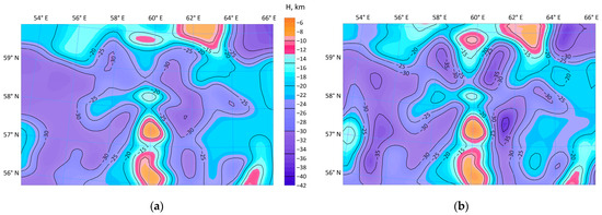
Figure 19.
Middle crust boundary: (a) initial position; (b) refined with GLCM.
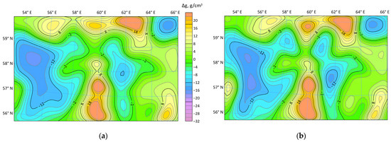
Figure 20.
Middle crust boundary fields: (a) for the initial boundary position; (b) corrected with anomaly field of the masses located in the depth range of (39, 49) km.
5. Discussion
The obtained results demonstrate the ability of the generalized local corrections method to be applied to practical problems.
The most indicative model example is example 5, which clearly demonstrates how crucial it is to ensure a good (geologically correct) approximation for the initial boundary in the local corrections method. It was also visible that the lack of some data in the initial approximation may lead to less distinct geometry features in resulting boundary, so it is very important to use all the existing data.
The method can be integrated with any a priori geophysical data if these data can be used to construct the initial approximation of the boundary. We use integration with seismic data, but the initial boundary could be constructed using data of other nature, such as thermal, magnetic, or magnetotelluric data. However, seismic boundaries are identified by the jump in wave propagation speed, which is more closely related to the density jump than other physical parameters.
For the region of the Urals, two boundaries were constructed. Despite their initial approximations being taken from different sources, the overall approach is the same, and it can be applied to a wide range of gravity modelling tasks. The most computationally demanding problem is obtaining a set of observed gravity field recalculation results, but, once obtained, the field for sources at any depth range is calculated by simple arithmetic summation.
In conclusion, the GLCM proved the efficiency and importance of every aspect of the generalization and could be recommended for use instead of the “classical” local corrections method for structural gravity inversion problems.
Future research directions might include the automatic selection of the parameter. Currently it is selected manually through a trial-and-error approach. Investigating the dependence of on the depth and geometry of the boundary appears to be promising. Automating the selection of the is also interesting to enable its variation between iterations, aiming to accelerate convergence. Another challenge is the simultaneous restoration of multiple boundaries in a multilayered medium. Such studies have already been initiated [7,11]; however, a stable and reliable scheme applicable to arbitrary practical boundaries has yet to be developed.
Author Contributions
Conceptualization, A.T.; methodology, A.T. and I.L.; software, A.T.; resources, I.L.; writing—original draft preparation, A.T. All authors have read and agreed to the published version of the manuscript.
Funding
This research was funded by Russian Science Foundation, grant number 20-17-00058.
Data Availability Statement
The original contributions presented in this study are included in the article. Further inquiries can be directed to the corresponding author.
Conflicts of Interest
The authors declare no conflicts of interest.
References
- Numerov, B.V. Interpretation of Gravitational Observations in the Case of a Contact Surface. Dokl. Akad. Nauk SSSR 1930, 21, 569. (In Russian) [Google Scholar]
- Tsuboi, C.; Fushida, T. Reations between gravity values and corresponding subterranean mass distribution. Bull. Earthq. 1937, 15, 636–649. [Google Scholar]
- Zamorev, A.A. On the definition of derivatives of the gravitational potential and of the relations between the moments of perturbing masses by a derivative given on a plane. Acad. Sci. U.R.S.S. Bull. Ser. Geol. Geophys. 1939, 3, 275–286. (In Russian) [Google Scholar]
- Strakhov, V.N. The inverse logarithmic-potential problem for a contact surface. Izv. Phys. Solid Earth 1974, 10, 104–114. [Google Scholar]
- Fedorova, N.V.; Tsirulskii, A.V. To the Solvability of the Inverse Problem of Logarithmic Potential for a Contact Surface in a Closed Form. Izv. Akad. Nauk SSSR 1976, 10, 61–72. (In Russian) [Google Scholar]
- Sultanov, M.A.; Akimova, E.N.; Misilov, V.E. Regularized gradient algorithms for solving the nonlinear gravimetry problem for the multilayered medium. Math. Method Appl. Sci. 2020, 45, 8760–8768. [Google Scholar]
- Prutkin, I.L. The solution of three-dimensional inverse gravimetric problem in the class of contact surfaces by the method of local corrections. Izv. Phys. Solid Earth 1986, 22, 49–55. [Google Scholar]
- Prutkin, I.; Saleh, A. Gravity and magnetic data inversion for 3D topography of the Moho discontinuity in the northern Red Sea area, Egypt. J. Geodyn. 2009, 47, 237–245. [Google Scholar] [CrossRef]
- Vajda, P.; Prutkin, I.; Tenzer, R.; Jentzsch, G. Inversion of temporal gravity changes by the method of local corrections: A case study from Mayon volcano, Philippines. J. Volcanol. Geotherm. Res. 2012, 241–242, 13–20. [Google Scholar] [CrossRef]
- Prutkin, I. Gravitational and magnetic models of the core–mantle boundary and their correlation. J. Geodyn. 2008, 45, 146–153. [Google Scholar] [CrossRef][Green Version]
- Martyshko, P.S.; Ladovskiy, I.V.; Tsidaev, A.G. Constructional of Regional Geophysical Models Based on the Joint Interpretation of Gravity and Seismic Data. Izv. Phys. Solid Earth 2010, 46, 931–942. [Google Scholar] [CrossRef]
- Nagy, D. The gravitational attraction of a right rectangular prism. Geophysics 1966, 31, 362–371. [Google Scholar] [CrossRef]
- Martyshko, P.; Ladovskii, I.; Byzov, D. Parallel Algorithms for Solving Inverse Gravimetry Problems: Application for Earth’s Crust Density Models Creation. Mathematics 2021, 9, 2966. [Google Scholar] [CrossRef]
- Laske, G.; Masters, G.; Ma, Z.; Pasyanos, M. Update on CRUST 1. 0—A 1-degree global model of Earth’s crust. Geophys. Res. Abstr. 2013, 15, 2658. [Google Scholar]
- Ladovskii, I.V.; Martyshko, P.S.; Tsidaev, A.G.; Kolmogorova, V.V.; Byzov, D.D. Lithosphere Density Model of the Middle Urals Segment. Izv. Phys. Solid Earth 2023, 59, 160–174. [Google Scholar] [CrossRef]
- Byzov, D.D.; Martyshko, P.S.; Ladovskii, I.V.; Tsidaev, A.G. 3D Seismic density models of the Earth’s crust and structural diagrams of tectonic zoning of the Middle Urals. Russ. Geol. Geophys. 2024, 65, 1240–1251. [Google Scholar] [CrossRef]
Disclaimer/Publisher’s Note: The statements, opinions and data contained in all publications are solely those of the individual author(s) and contributor(s) and not of MDPI and/or the editor(s). MDPI and/or the editor(s) disclaim responsibility for any injury to people or property resulting from any ideas, methods, instructions or products referred to in the content. |
© 2024 by the authors. Licensee MDPI, Basel, Switzerland. This article is an open access article distributed under the terms and conditions of the Creative Commons Attribution (CC BY) license (https://creativecommons.org/licenses/by/4.0/).

