Abstract
This study proposes a nonlinear adaptive optimal control method, the adaptive H2 control method, applied to the trajectory tracking problem of the wheeled mobile robot (WMR) with four-wheel mecanum wheels. From the perspective of solving mathematical problems, finding an analytical adaptive control solution that satisfies the adaptive H2 performance criterion for the trajectory tracking problem of the WMR with four-wheel mecanum wheels is an extremely challenging task due to the high complexity of the dynamic system. To analytically derive the control law and adaptive control law for this trajectory tracking problem, a proportional-derivative (PD) type transformation is employed to formalize the trajectory tracking error dynamics between the WMR and the desired trajectory (DT). Based on an in-depth analysis of the trajectory tracking error dynamics, a closed-form adaptive control law is analytically derived from the highly complex nonlinear dynamic system equations. This control law provides a solution to the trajectory tracking problem of the WMR while satisfying the adaptive H2 performance criterion. The proposed adaptive nonlinear control method offers a simple control structure and advantages such as improved energy efficiency. Finally, simulations and experimental implementations were conducted to verify the performance of the proposed adaptive H2 control method and the H2 control method in tracking the DT. The results demonstrate that, compared to the H2 control method, the adaptive H2 control method exhibits superior trajectory tracking performance, particularly in the presence of significant model uncertainties.
Keywords:
trajectory tracking; adaptive H2 control method; mecanum wheels; adaptive H2 performance criterion; energy consumption MSC:
37M05
1. Introduction
In recent years, WMRs have attracted significant attention due to their extensive applications across industrial, commercial, domestic, educational, military, and agricultural sectors. These applications predominantly involve areas such as goods transportation, navigation services, household cleaning, educational entertainment, patrol inspection, and agricultural assistance [1,2,3,4,5,6,7,8]. However, to function effectively in shifting surroundings, these WMRs must fulfill criteria for protection, precision, robustness, and excellent agility to enable accurate autonomous movement. Currently, many WMRs utilize either a two-wheel drive system with an additional omnidirectional wheel or a four-wheel mecanum drive system to meet the demands of these applications. The key enabling technology to fulfill these tasks is a control method ensuring accurate trajectory tracking. This study reviews recent advancements in the field, including model-free adaptive control [9], finite-time control [10,11], backstepping control [12,13,14,15], PID control [16,17,18,19,20], sliding mode control [21,22,23,24,25,26,27], fuzzy control [28,29,30], neural network control [31,32,33,34], H2 control [35,36], and feedback linearization control [37,38,39]. These simulation-based studies primarily focus on trajectory tracking control designs for wheeled mobile robots (WMRs) equipped with either mecanum or non-mecanum wheels in two-wheel or four-wheel drive configurations. Addressing the issue of model uncertainties in WMRs, several studies [9,10,11,12,15,21,22,24,28,29,30,40] have employed adaptive control methods to tackle the challenges posed by such uncertainties. Model uncertainties are a critical issue for WMRs, as neglecting them in control design can, under certain conditions, degrade tracking accuracy, increase the computational burden of the controller, and result in higher energy consumption. To meet the demands of practical applications, it is therefore essential to develop WMRs with energy-efficient and precise trajectory tracking capabilities, alongside robust handling of model uncertainties. Consequently, designing a simple yet optimized control architecture and developing a high-performance optimization control method are crucial for WMRs. Moreover, achieving these desired characteristics requires deriving an analytical solution to the nonlinear optimal trajectory tracking problem.
References [35,36] presents a WMR nonlinear optimal control analytical solution based on a coordinate transformation approach for fixed system parameters. However, solving the nonlinear optimal trajectory tracking problem for WMRs presents a highly challenging task, and deriving an analytical solution for WMR trajectory tracking remains difficult, even mathematically. The H2 control method proposed in [35,36] demonstrates that, through appropriate arrangement of the mathematical model, an optimal trajectory tracking analytical solution can be obtained for a WMR with fixed system parameters. This result provides an analytical solution for trajectory tracking in WMRs with fixed parameters. However, WMRs with fixed system parameters are exceptional cases; parameters such as mass and inertia can vary significantly due to changes in load and energy loss. To address this limitation of the H2 control method in [35,36], which does not account for variations in system parameters, this study proposes an adaptive H2 optimization control method to enhance the accuracy and performance of trajectory tracking for a four-wheel mecanum-wheeled mobile robot under model uncertainty. Based on the above discussion, this study employs both simulation and practical implementation of a four-wheel mecanum-wheeled mobile robot to validate the trajectory tracking performance of the H2 control method and the proposed adaptive H2 optimization control method.
This paper is structured as follows: Section 1 introduces the background and literature review; Section 2 describes the mathematical model of the WMR and the tracking error dynamics between the desired and actual trajectories; Section 3 introduces the proposed nonlinear adaptive optimal control design based on the adaptive H2 performance criterion; Section 4 demonstrates the simulation verifications of trajectory tracking based on the proposed method; Section 5 presents experimental results of the implemented WMR tracking the DT; and Section 6 concludes the findings of this study.
2. Mathematical Model of the WMR
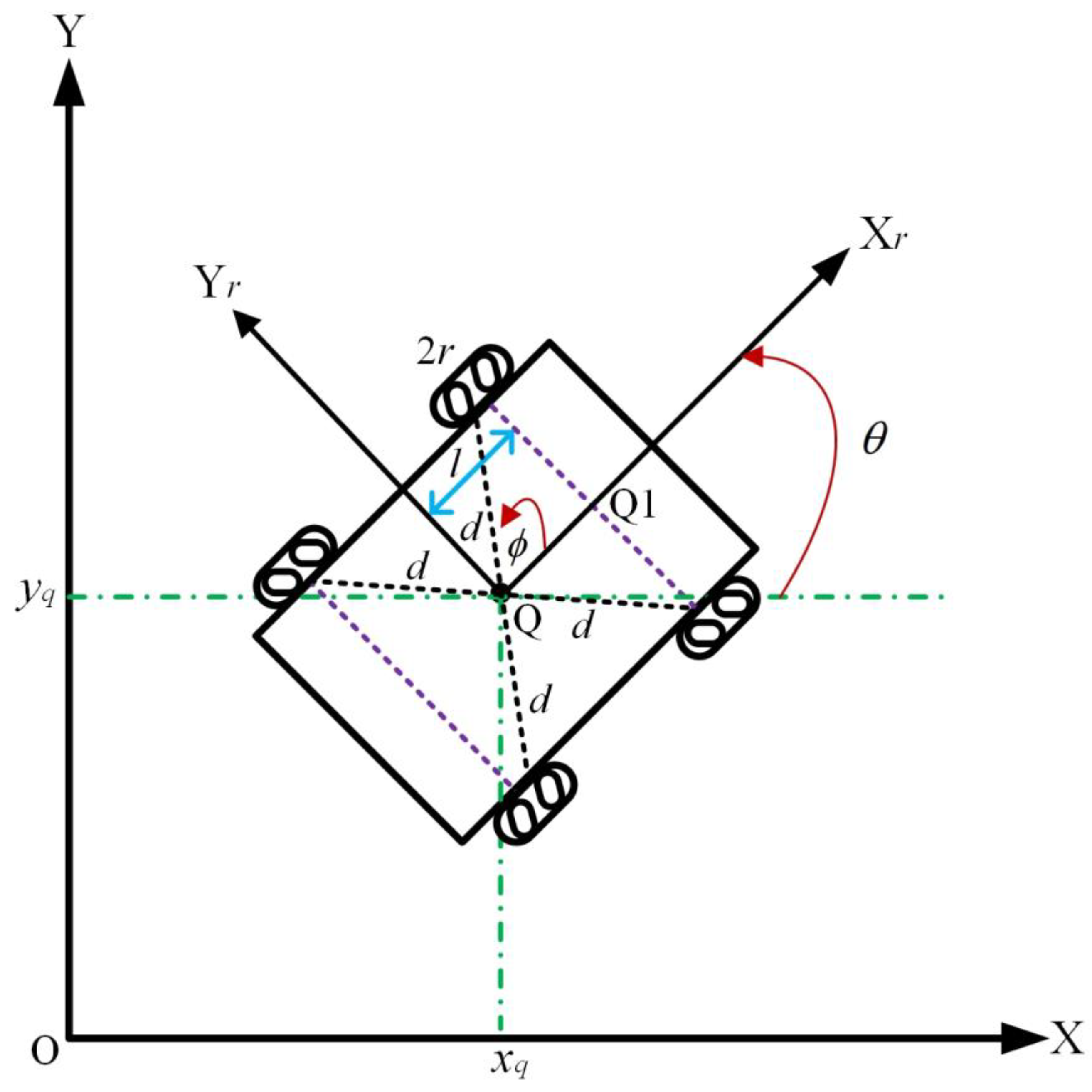
This section explains the dynamic equations of the WMR and the dynamic equations for the DT tracking error. The WMR is equipped with four mecanum driving wheels. Each mecanum wheel contains a set of passive rollers that rotate around the hub of the robot. Figure 1 illustrates the schematic diagram of the WMR equipped with four mecanum driving wheels [39]. The relevant parameters, dynamic equations, and the dynamic equations for the DT tracking error of the WMR will be detailed in the following sections.

Figure 1.
Schematic diagram of the WMR equipped with four mecanum driving wheels.
2.1. The Dynamic Equations of WMR
From Figure 1, schematic diagram of the WMR equipped with four mecanum driving wheels, the following parameters related to the WMR are described: X, Y represent the global coordinate system; Xr, Yr represent the moving coordinate system associated with the WMR at point Q; l represents the distance between positions Q and Q1; d denotes the distance between the center point Q and the mecanum wheel; represents the rotation angle of the WMR; represents the rotation angle between the roller axis and the wheel plane.
As illustrated in Figure 1, the WMR usually moves along the orientation of the axis of the driving wheels, and its dynamic equations can be described as in Equation (1) [39]. Based on the previous explanations, the global coordinate system of the WMR is represented by Equation (2).
where
where represents the inertia matrix, represents the Coriolis and centripetal matrix, represents the generalized velocity vector, represents the generalized acceleration vector, represents the input transformation matrix, represents the friction direction matrix, represents the wheel rotational speed, represents the friction effect matrix, r represents the wheel radius, represents the moment of force vector, represents the platform mass, represents the wheel mass, represents the platform moment of inertia, and Iw represents the wheel moment of inertia. In this study, the WMR parameters (,,) are subject to uncertainties due to model perturbations that account for variations in payload.
2.2. Dynamic Equations of Trajectory Tracking Error for WMR
Suppose the related DT used in this study is a twice continuously differentiable function . Let and represent the velocity and acceleration vectors of the desired tracking trajectory, respectively. Therefore, the tracking error of the controlled WMR’s trajectory can be represented as:
where
Based on Equations (1) and (10), the dynamics of the trajectory tracking error are given by:
From a mathematical viewpoint, addressing the trajectory tracking problem of the controlled WMR through Equation (12) is particularly challenging due to the complex structure of the error dynamics between the WMR and the DT. To alleviate the design complexity of the proposed closed-form control method, a PD transformation is incorporated, aiming to simplify the derivative-related aspects of the control design. The following equation represents the PD transformation introduced in this approach.
where and are positive constants.
The differentiation of Equation (13), we can obtain the following:
where
Using Equation (14), the trajectory tracking error dynamics in Equation (12) can be reformulated to incorporate a parameterized term Ω(t)Λ(t), enabling accurate estimation of the disturbed system parameters , , and . Accordingly, the revised dynamics of the trajectory tracking error are expressed in Equation (18).
where
and represents the state-space transformation matrix, defined as follows:
If is selected by Equation (24)
then the adjusted dynamic equation for the trajectory tracking error is reformulated as follows:
where denotes the parameter estimation error.
3. Nonlinear Adaptive Optimal Control Design
In this section, an analytic nonlinear adaptive optimal H2 control method that satisfies the adaptive H2 control performance criterion will be derived for trajectory tracking of the WMR. This nonlinear adaptive optimal H2 control method consists of two parts: the adaptive control law and the adaptive law. The following sections will provide a detailed explanation of the adaptive H2 trajectory tracking control design and the analytical solution for adaptive H2 control design.
3.1. Adaptive H2 Trajectory Tracking Control Design
In examining the trajectory tracking error dynamics of the WMR as described in Equation (25), the aim is to formulate an adaptive H2 closed-form control law that fulfills the adaptive H2 performance criterion [40] specified in Equation (27). The trajectory tracking problem of the WMR is considered to be addressed if a closed-form solution and an adaptive law can be found that accomplish the adaptive H2 performance criterion for all .
where , , , and are predefined positive definite weighted matrices, , and .
According to the mathematical proof provided in Appendix A, if a unique solution can be identified for the following nonlinear, time-varying differential equation, the trajectory tracking problem of the WMR can be guaranteed to have an analytical solution. In this case:
and the associated control law can be expressed as follows:
where:
3.2. Analytical Solution for Adaptive H2 Control Design
By examining Equation (28), it becomes clear that the trajectory tracking problem can be analytically resolved if the closed-form solution is mathematically determined. Due to the complexity and time-varying nature of this differential equation, obtaining the analytical solution for Equation (28) is a challenging task. However, an analytical solution can be constructed by appropriately choosing in the following form.
where and denote adjustable positive matrices, the values of which will be determined in accordance with particular conditions.
By applying Equation (18) along with from Equation (33), we obtain:
where:
Applying Equations (20) and (33), Equation (36) can be obtained:
From Equations (34) and (36), the Equation (28) can be expressed as follows:
Hence:
where , the symmetric matrix that is positive definite in Equation (37) is represented in diagonal form and can be additionally factored in the following manner:
Employing and B together, as specified in Equations (21) and (22), Equation (37) can be detailed as follows:
According to Equation (22), the sub-matrices and can be derived as shown below:
Hence:
To meet conditions and in Equation (22), the weighting matrices and in Equation (40) must be in diagonal form, which is expressed as:
By employing the results obtained from Equation (37), the adaptive control law for the WMR can be formulated as detailed in Equation (46):
In addition, the adaptive law for the WMR is derived as follows:
Consequently, the trajectory tracking problem of the adaptive H2 closed-form control method can be addressed using the following adaptive H2 control law:
4. Simulation Verification
In this study, we utilized the software MATLAB R2021b to simulate and validate the trajectory tracking performance of the H2 and adaptive H2 control methods for the DTs of a 100 m × 30 m rectangular trajectory and a double triangle trajectory with a base length of 200 m. The following section presents the simulation configurations and discusses the results for tracking the DTs.
4.1. Simulation Configurations
The configurations of the WMR and the assumed values for modeling uncertainties are presented, with the corresponding parameter values listed below in this section.

Table 1.
The configurations of the controlled WMR [41].
For this controlled WMR, the modeling uncertainties are assumed to be 20% of the mass , distance and inertia . The time-varying mass is defined as a fixed value combined with a varying component , the time-varying distance is defined as a fixed value combined with a varying component and the time-varying inertia is defined as a fixed value combined with a varying component . The varying components , and represent 20% variations of , and , respectively, to simulate the practical scenarios of the WMR carrying different loads.
4.2. Simulation Results
In this study, two simulation scenarios were used to compare the trajectory-tracking performances between the H2 control method and the proposed adaptive H2 control method. The DTs for these two scenarios consist of a 100 m × 30 m rectangular trajectory and a double triangle trajectory with a base length of 200 m. The detailed settings and simulation comparison results for these two scenarios are described as follows.
4.2.1. Scenario 1 (Rectangular Trajectory)
In this simulation, a DT was created using 27 waypoints, as outlined in Table 2. After establishing the DT, the controlled WMR used the H2 and adaptive H2 control methods to perform trajectory tracking. The DT consists of straight segments and multiple turns, intended to assess the performance of the H2 and adaptive H2 control methods in trajectory tracking.
Table 2.
Waypoints of scenario 1.
Table 3 provides the initial conditions of the controlled WMR used in this scenario 1.
Table 3.
Initial conditions for scenario 1.
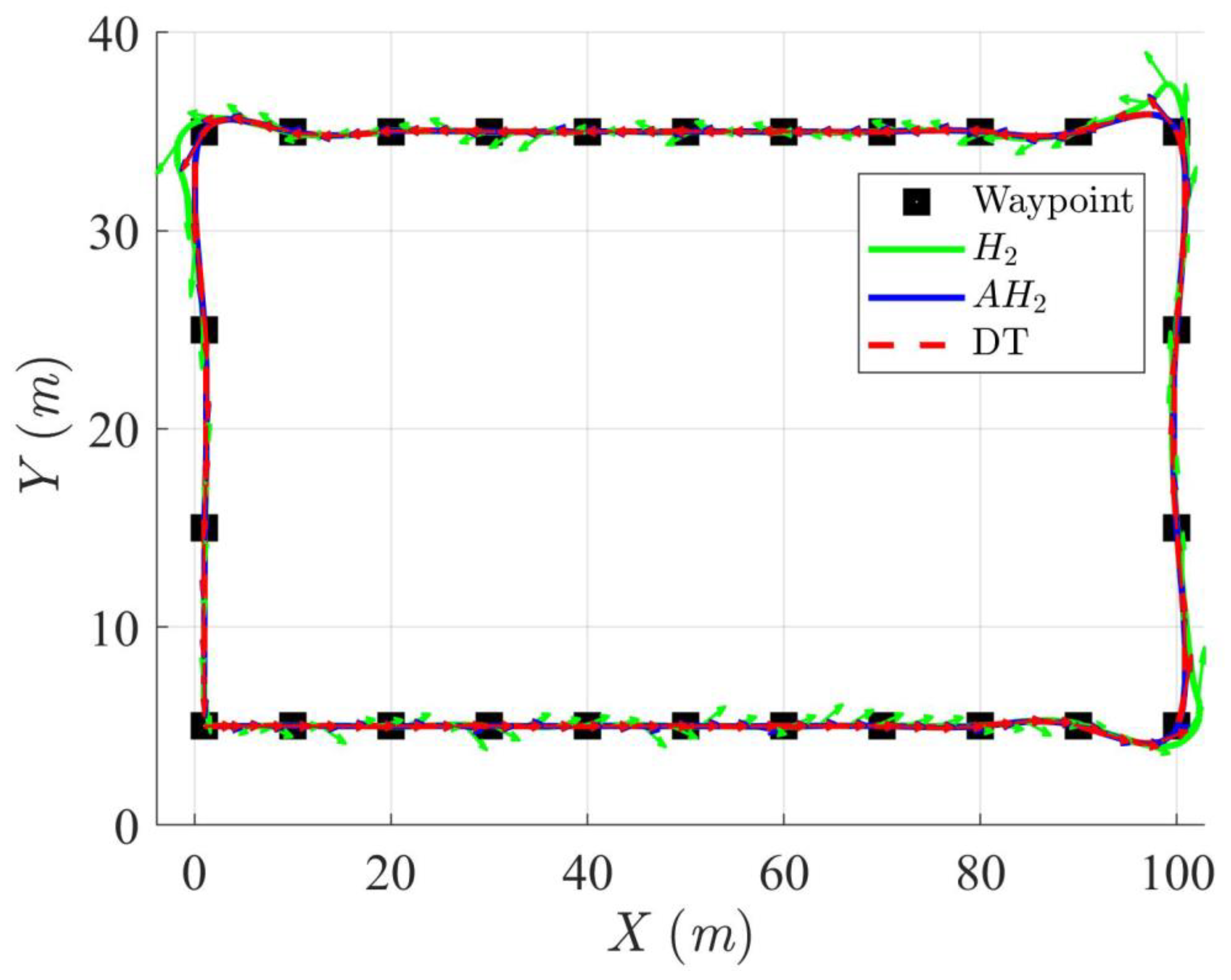
Simulation results in Figure 2, Figure 3, Figure 4 and Figure 5 illustrate the trajectory and pose tracking of DT under the influence of limited modeling uncertainties, using both the H2 and adaptive H2 control methods. Figure 6, Figure 7 and Figure 8 present the tracking errors in the XY plane as well as heading angle errors associated with these methods. Analysis reveals that the H2 control method exhibits greater tracking errors, whereas the adaptive H2 control method achieves smaller, acceptable errors. The findings clearly show that the adaptive H2 control method is more robust against modeling uncertainties, achieving higher precision in trajectory tracking. In Figure 2, Figure 5 and Figure 8, the heading angle of the WMR controlled by the H2 method fluctuates noticeably, especially at turning points, reflecting the H2 method’s limitations in effectively guiding the WMR along the DT in the presence of uncertainties. Conversely, the adaptive H2 control design maintains close alignment with the DT path. Furthermore, control torques depicted in Figure 9, Figure 10 and Figure 11 demonstrate that the adaptive H2 control method requires lower torque than the H2 method. These findings demonstrate that the adaptive H2 control method not only swiftly aligns the WMR with the desired heading but also optimally produces control torque to maintain precise heading during trajectory tracking, thereby enhancing energy efficiency. In conclusion, the simulation results validate that the adaptive H2 control method outperforms the H2 control method in both trajectory and pose tracking performance for the WMR in this scenario. Significantly, the adaptive H2 method produces control outputs similar to those of the H2 method, delivering superior accuracy in trajectory tracking.
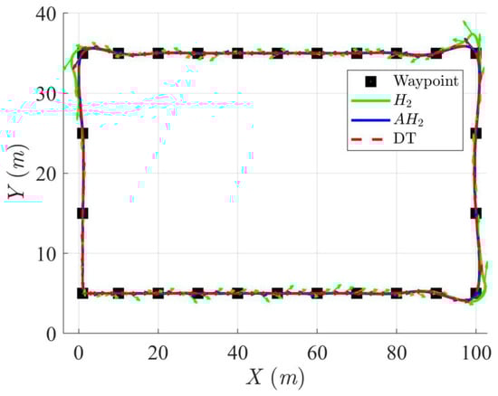
Figure 2.
Trajectory tracking of DT and orientation of the controlled WMR using H2 and adaptive H2 (AH2) methods for scenario 1.
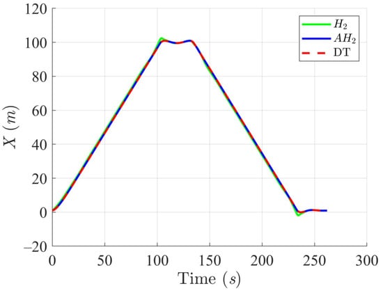
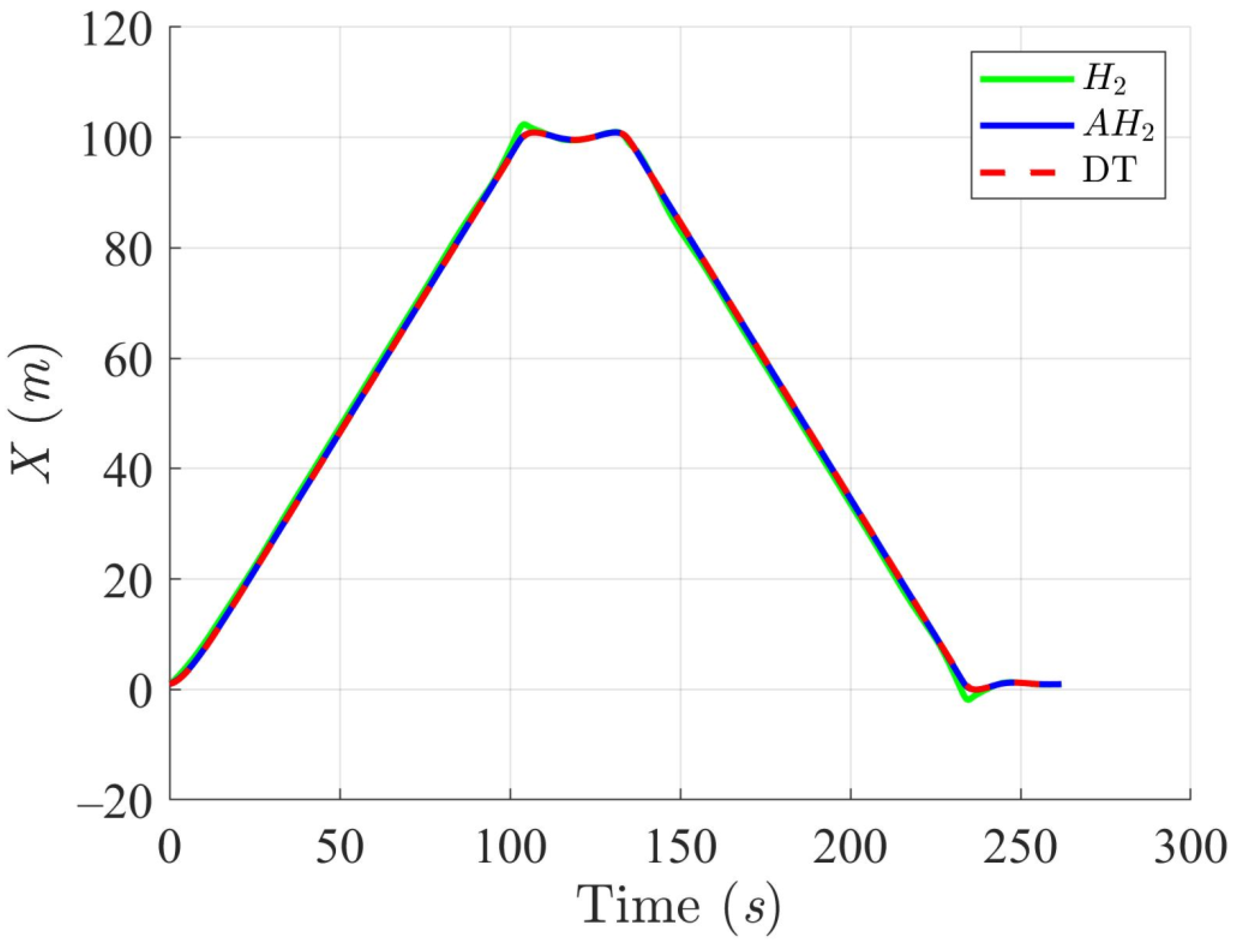
Figure 3.
Trajectory tracking results of the DT along the X-axis using H2 and adaptive H2 (AH2) methods for scenario 1.
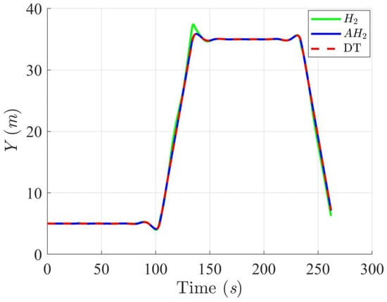
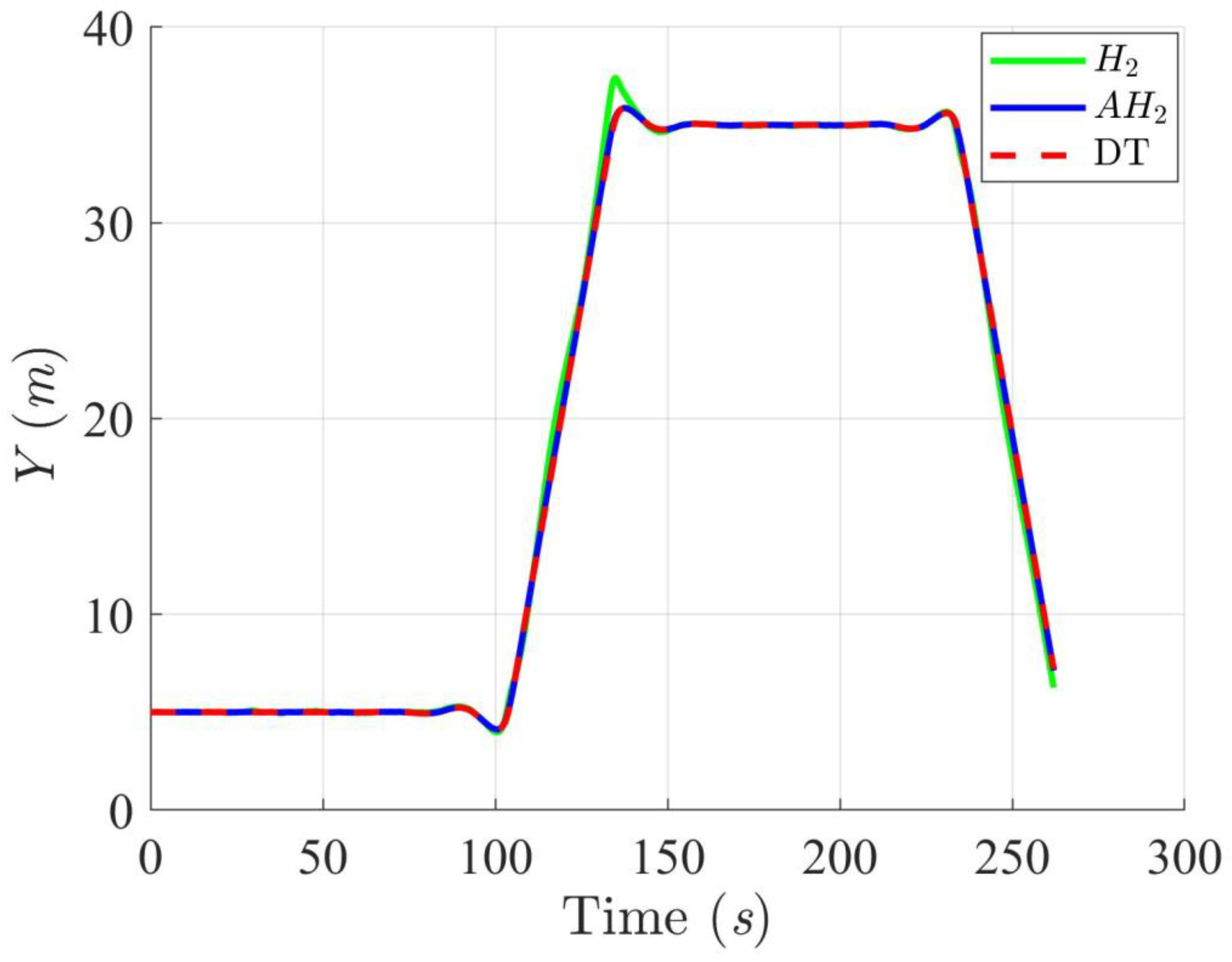
Figure 4.
Trajectory tracking results of the DT along the Y-axis using H2 and adaptive H2 (AH2) methods for scenario 1.
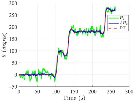
Figure 5.
Trajectory tracking results of the DT at an angle using H2 and adaptive H2 (AH2) methods for scenario 1.
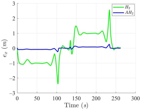
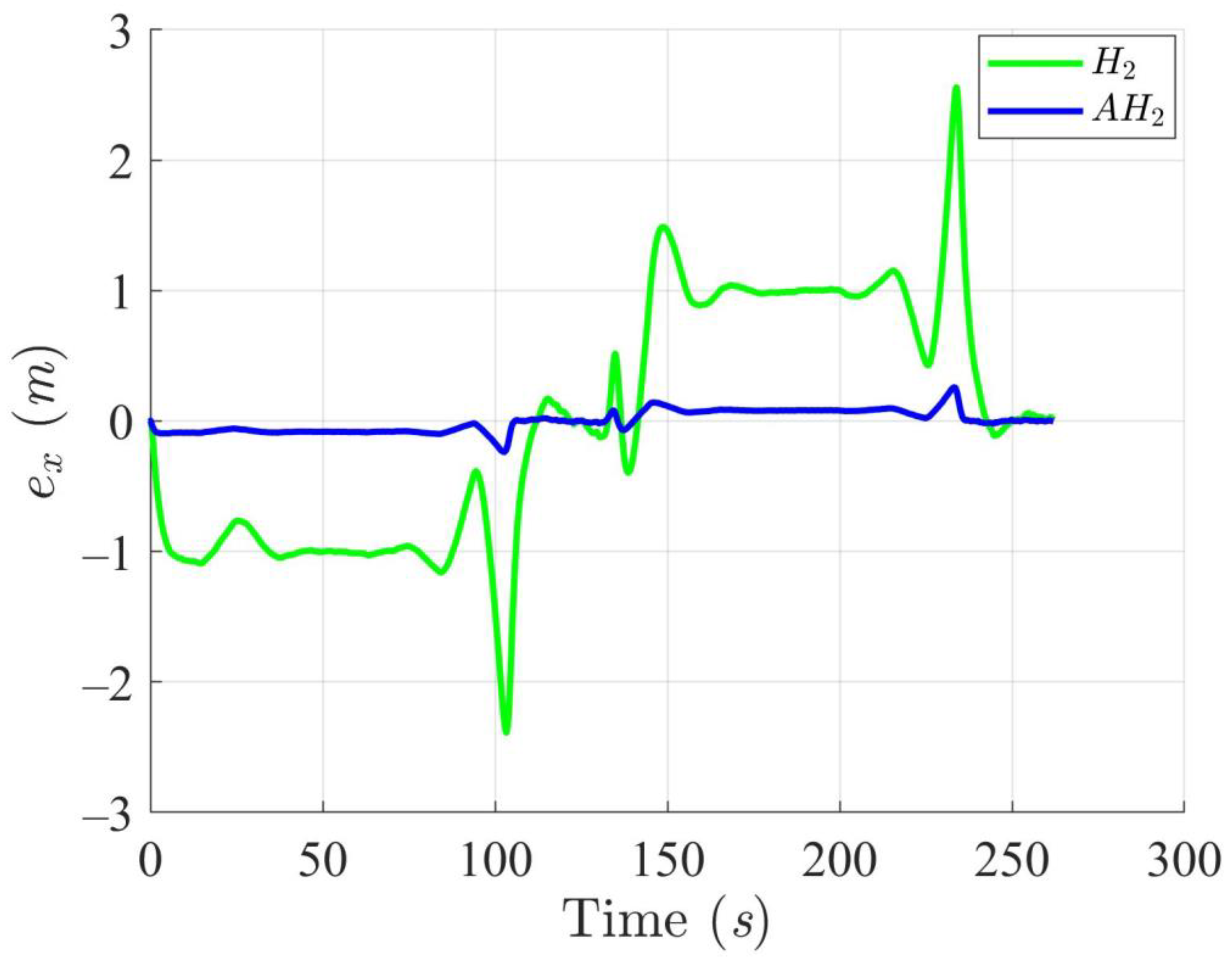
Figure 6.
Trajectory tracking errors along the X-axis utilizing the H2 and adaptive H2 (AH2) methods for scenario 1.
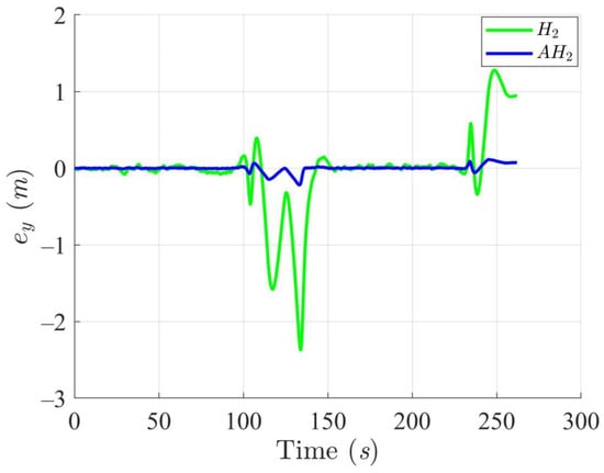
Figure 7.
Trajectory tracking errors along the Y-axis utilizing the H2 and adaptive H2 (AH2) methods for scenario 1.

Figure 8.
Trajectory tracking errors of heading angle utilizing the H2 and adaptive H2 (AH2) methods for scenario 1.
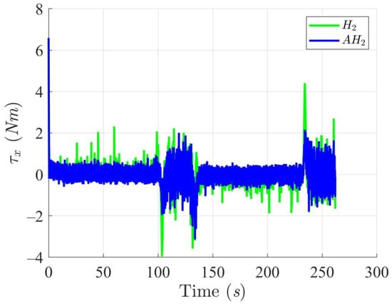
Figure 9.
Trajectory tracking torques along the X-axis utilizing the H2 and adaptive H2 (AH2) methods for scenario 1.
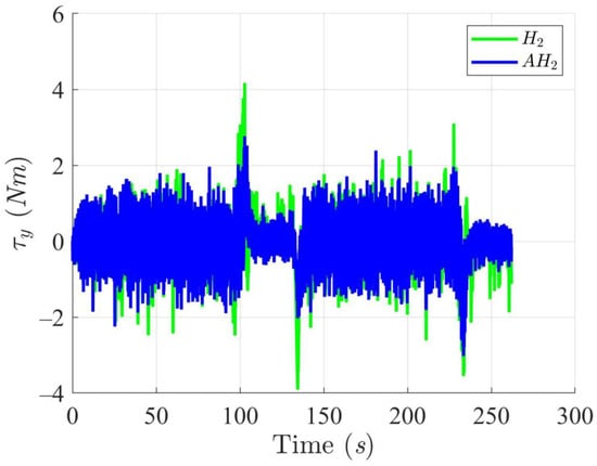
Figure 10.
Trajectory tracking torques along the Y-axis utilizing the H2 and adaptive H2 (AH2) methods for scenario 1.
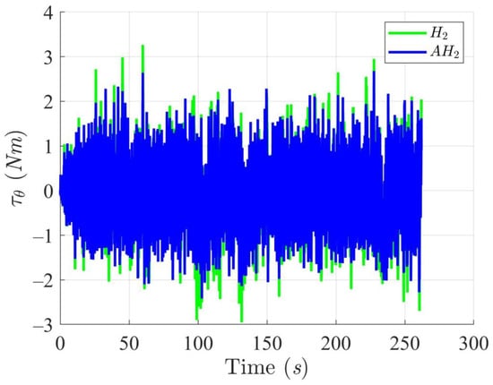
Figure 11.
Trajectory tracking torques on heading angle utilizing the H2 and adaptive H2 (AH2) methods for scenario 1.
4.2.2. Scenario 2 (Double Triangle Trajectory)
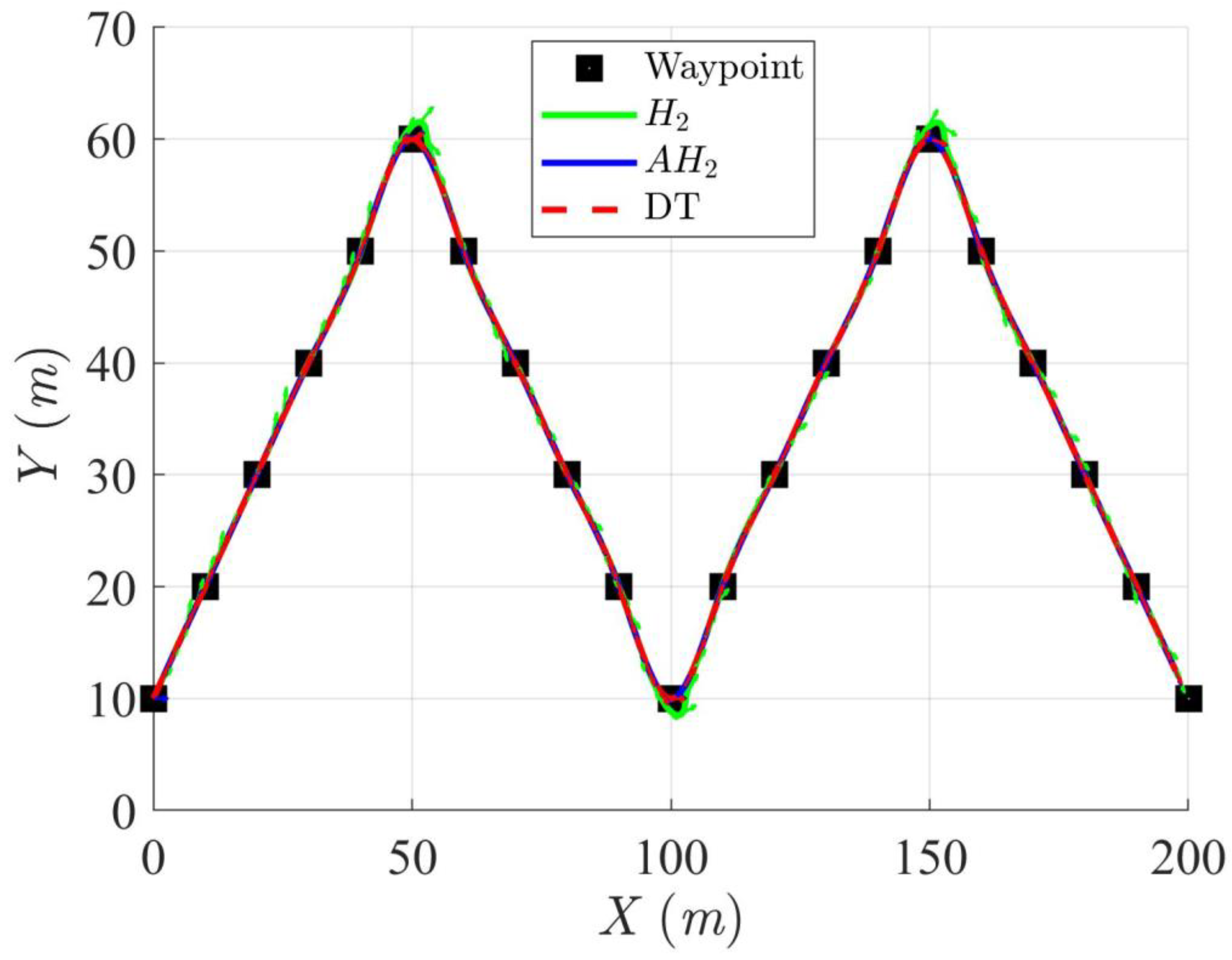
In this simulation scenario 2, a double triangle trajectory was created using 21 waypoints as shown in Table 4, serving as the DT for this scenario. This double triangle trajectory mainly consists of four straight segments and three sharp turns. After establishing this double triangle trajectory, the H2 and adaptive H2 control methods were used to compare their trajectory-tracking performance.
Table 4.
Waypoints of scenario 2.
Table 5 provides the initial conditions of the controlled WMR used in this scenario 2.
Table 5.
Initial conditions for scenario 2.
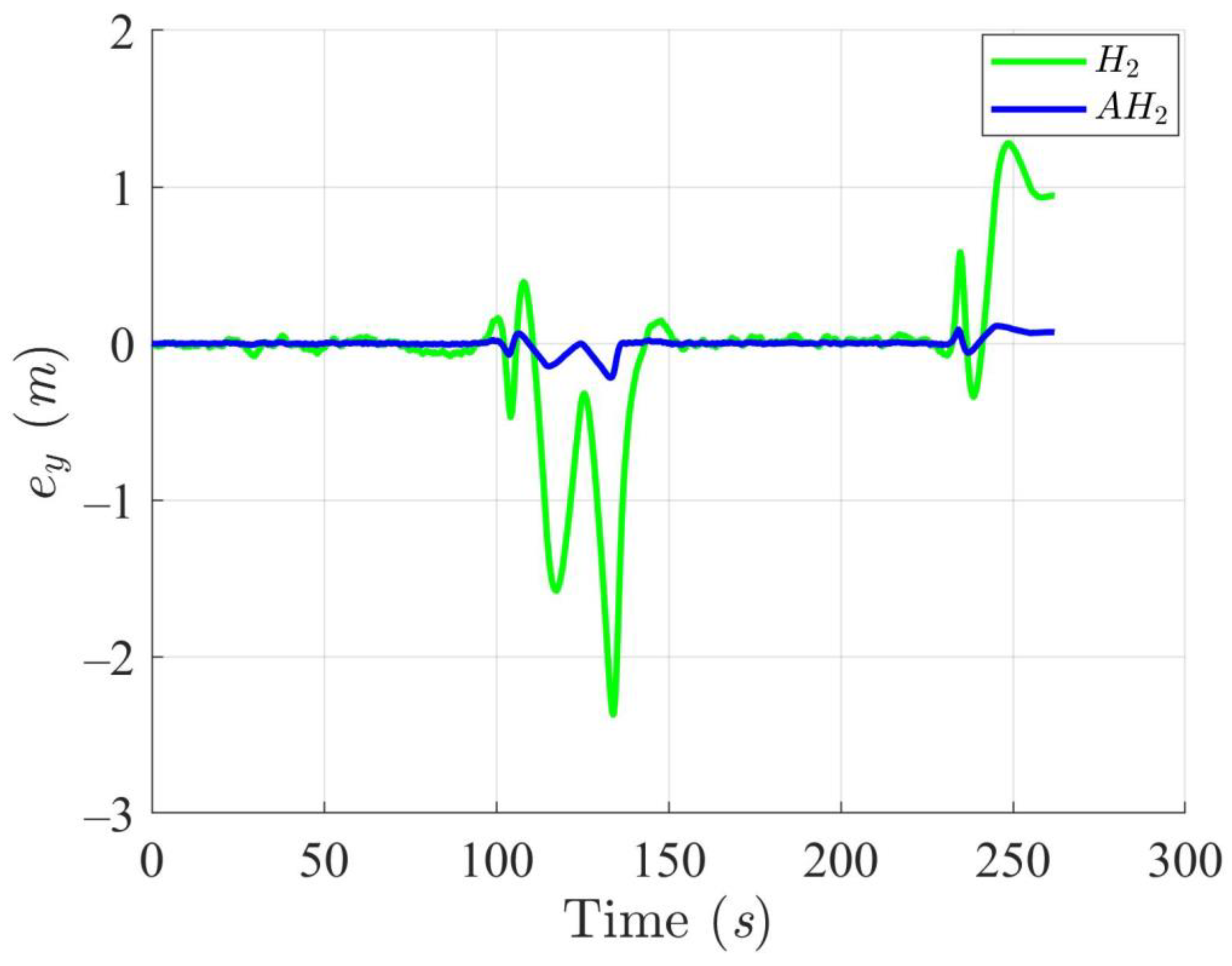
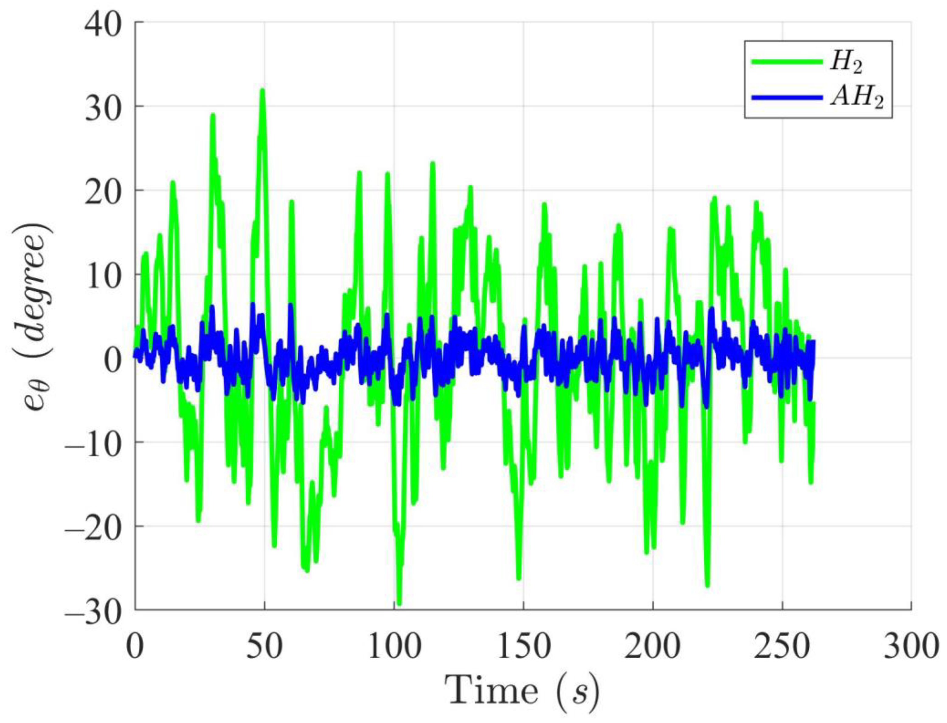
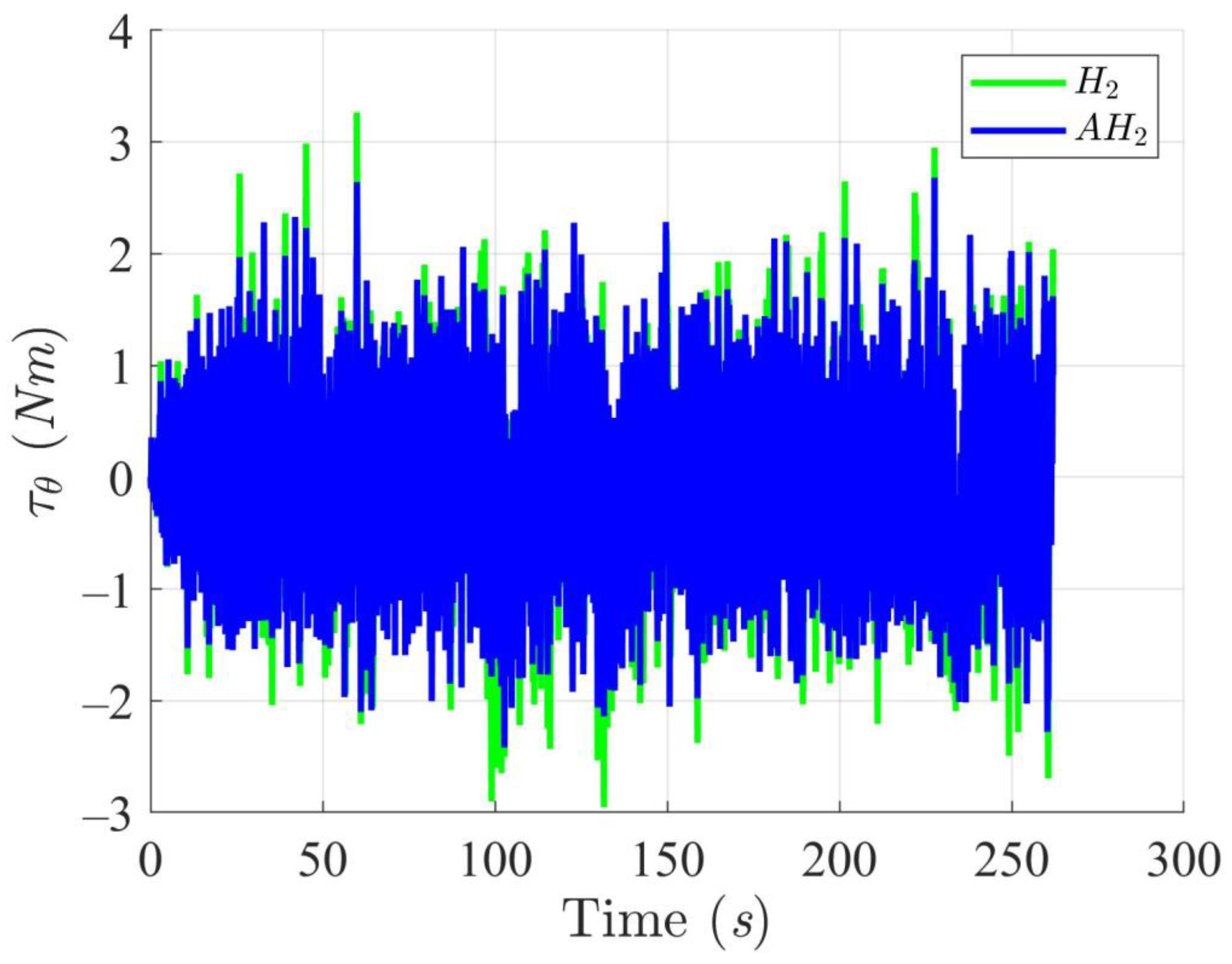
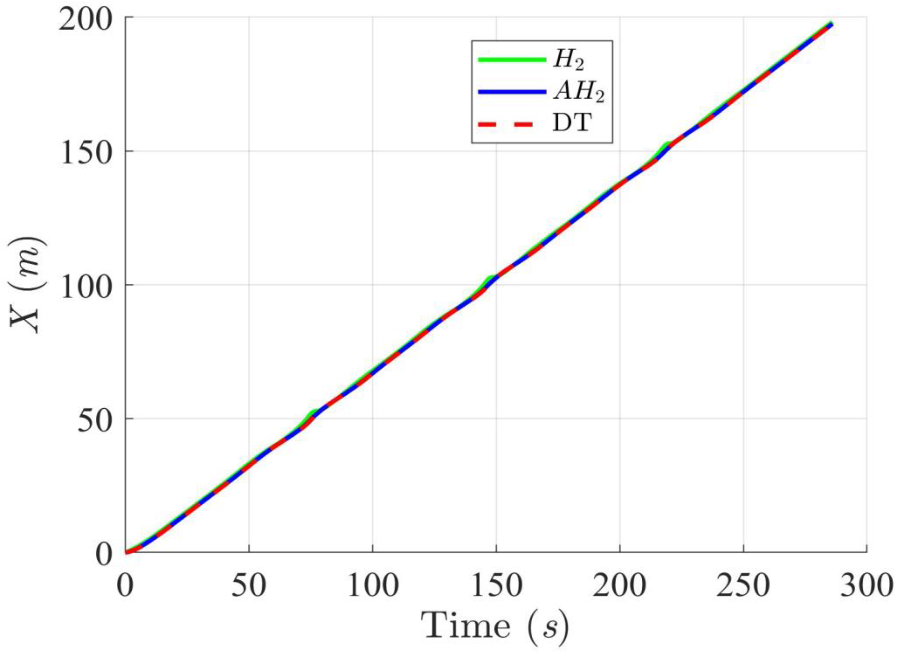
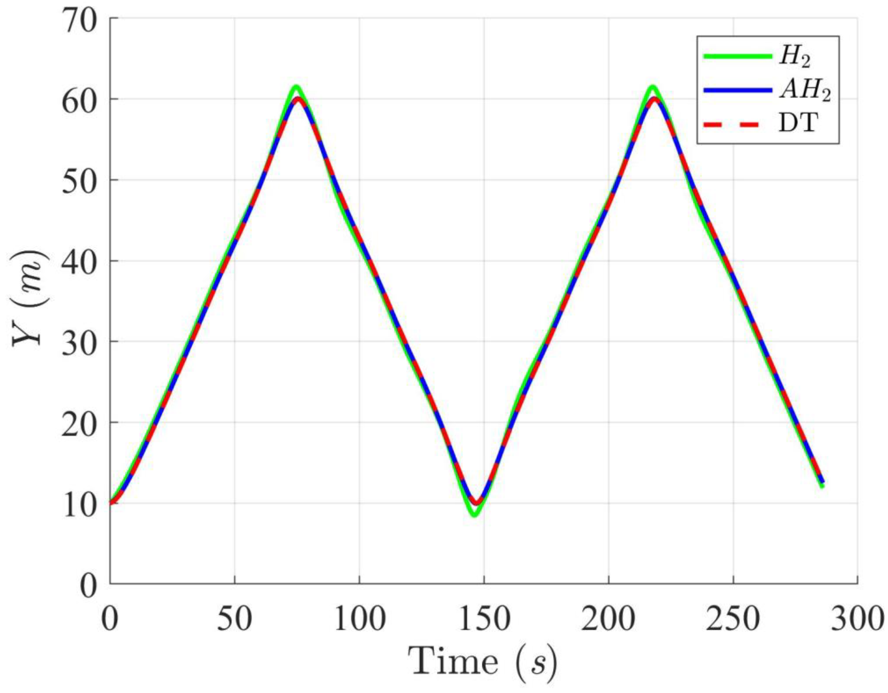
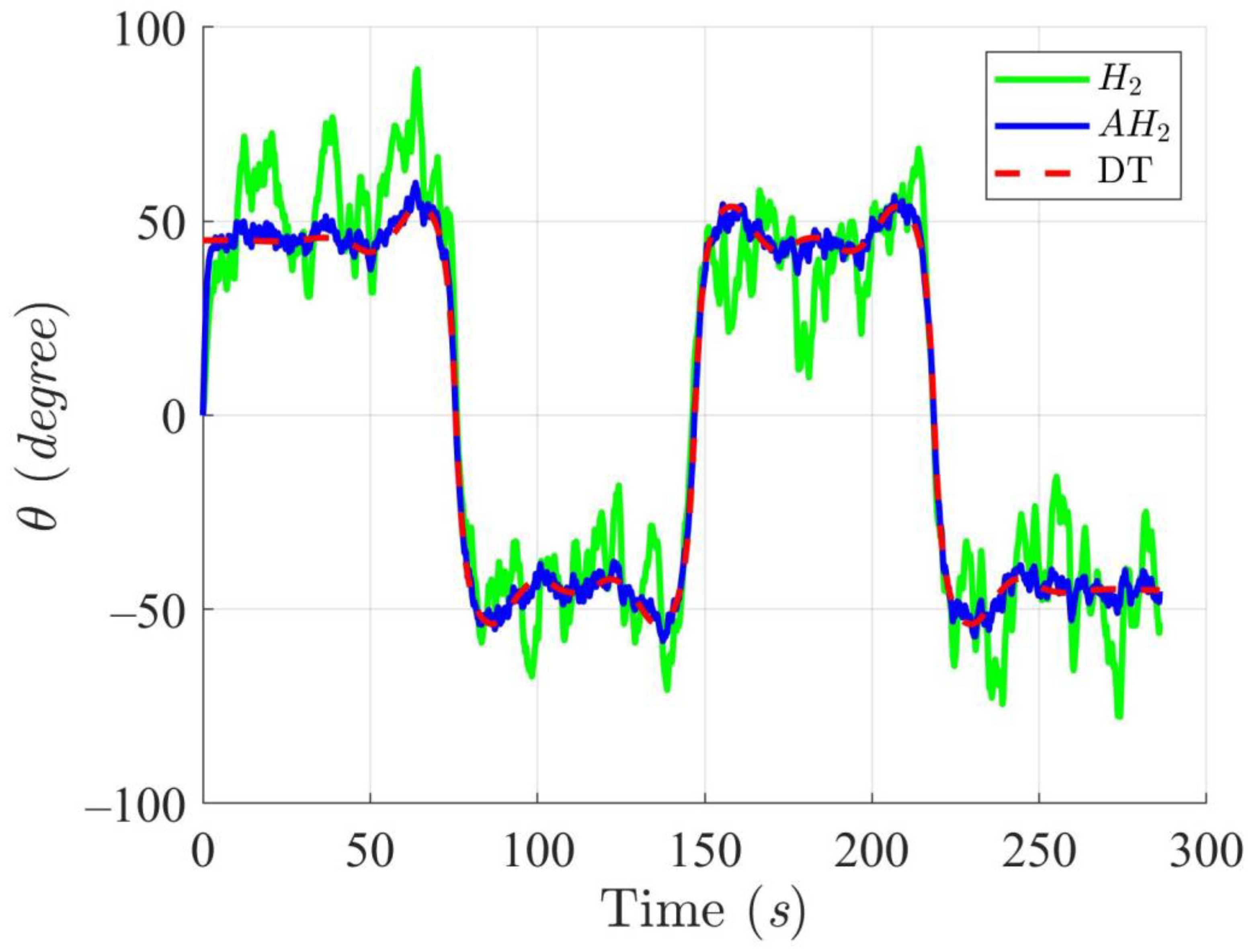
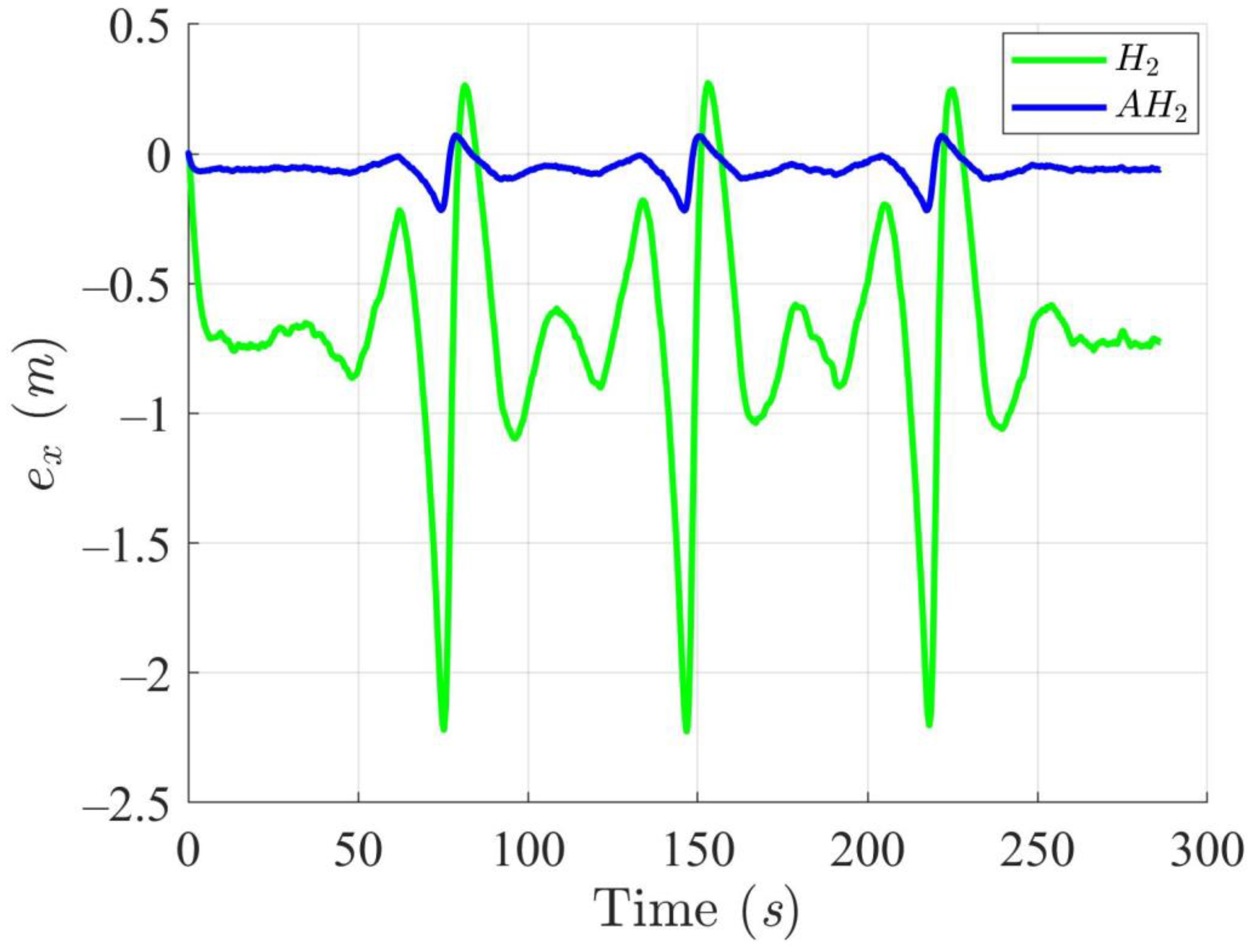
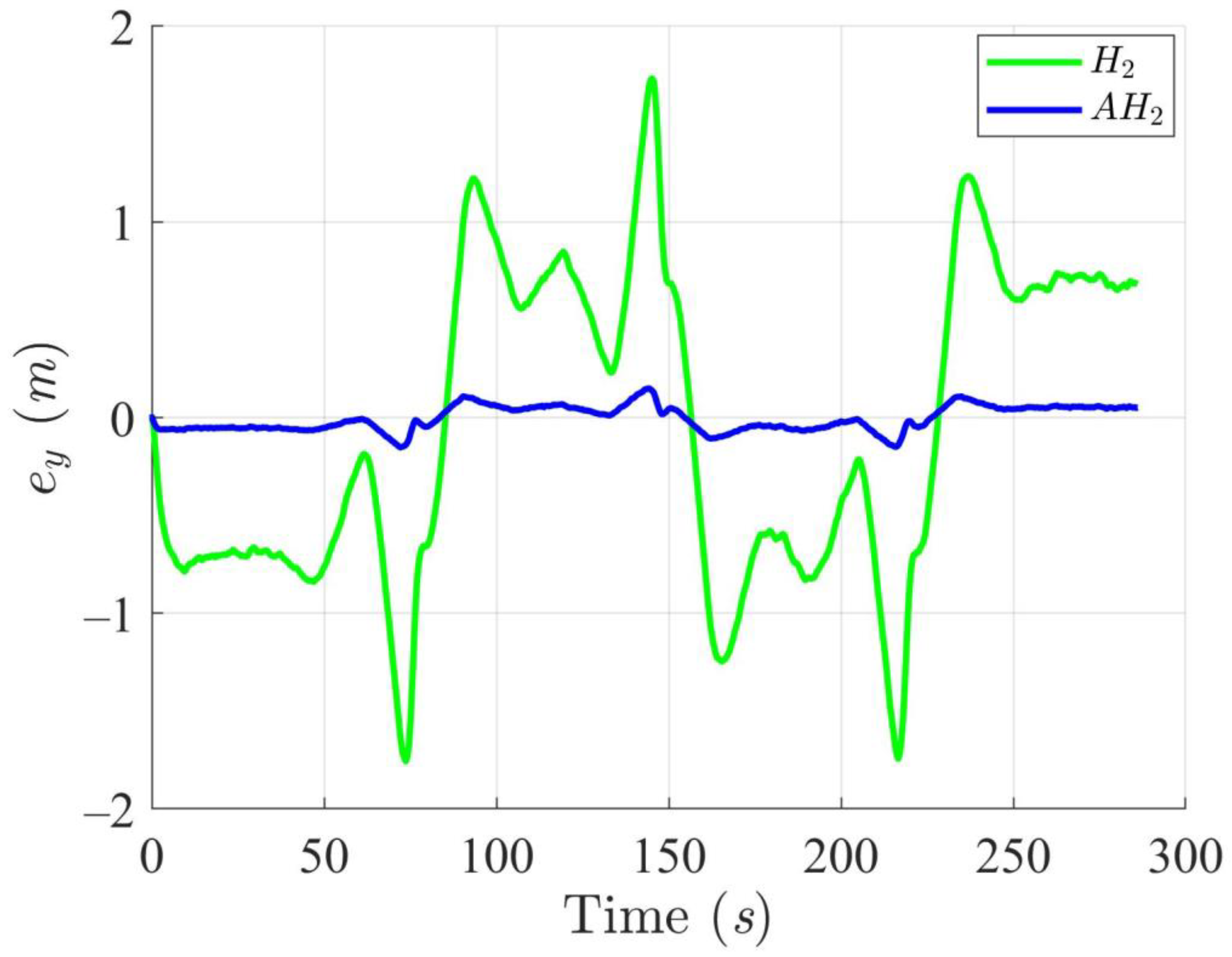
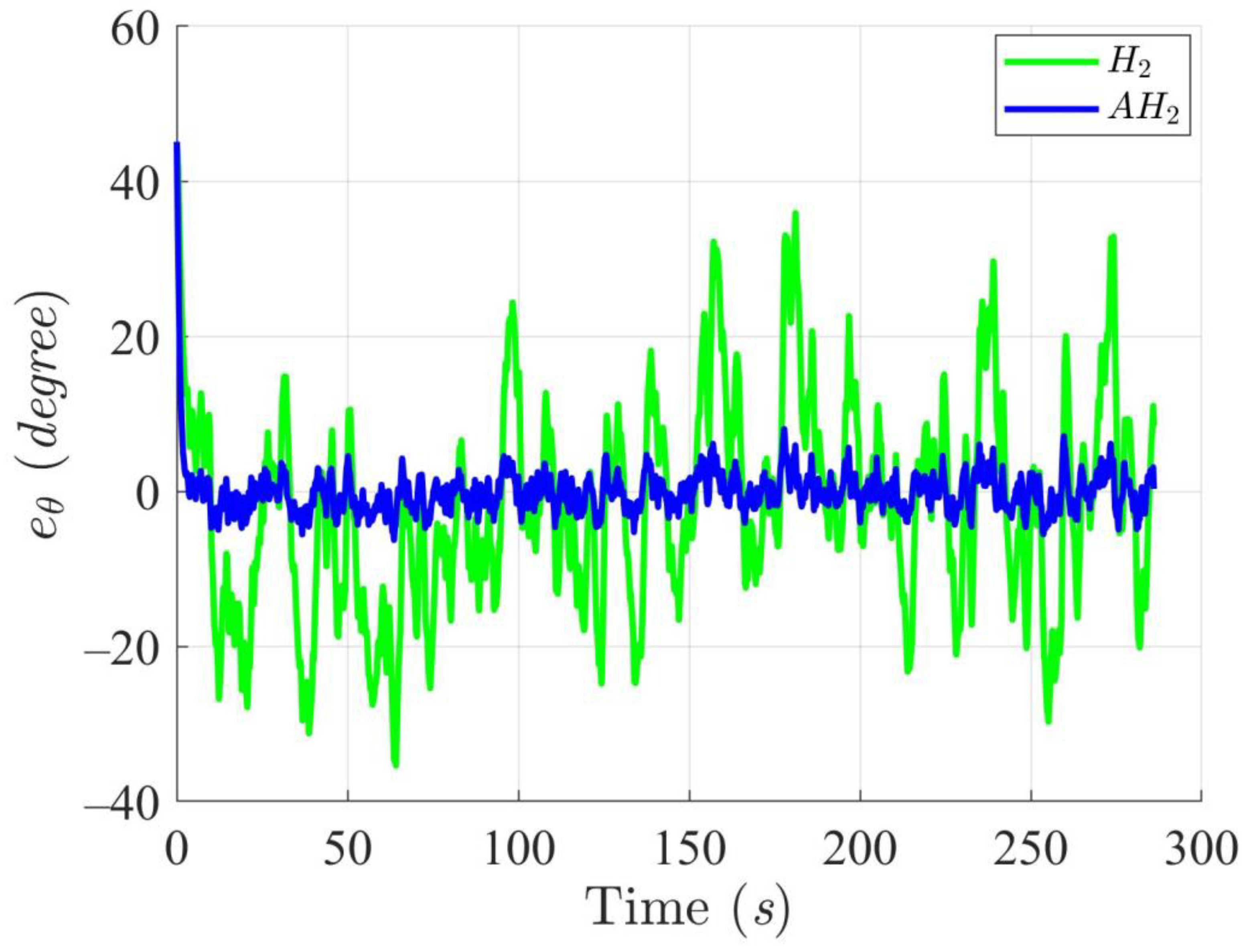
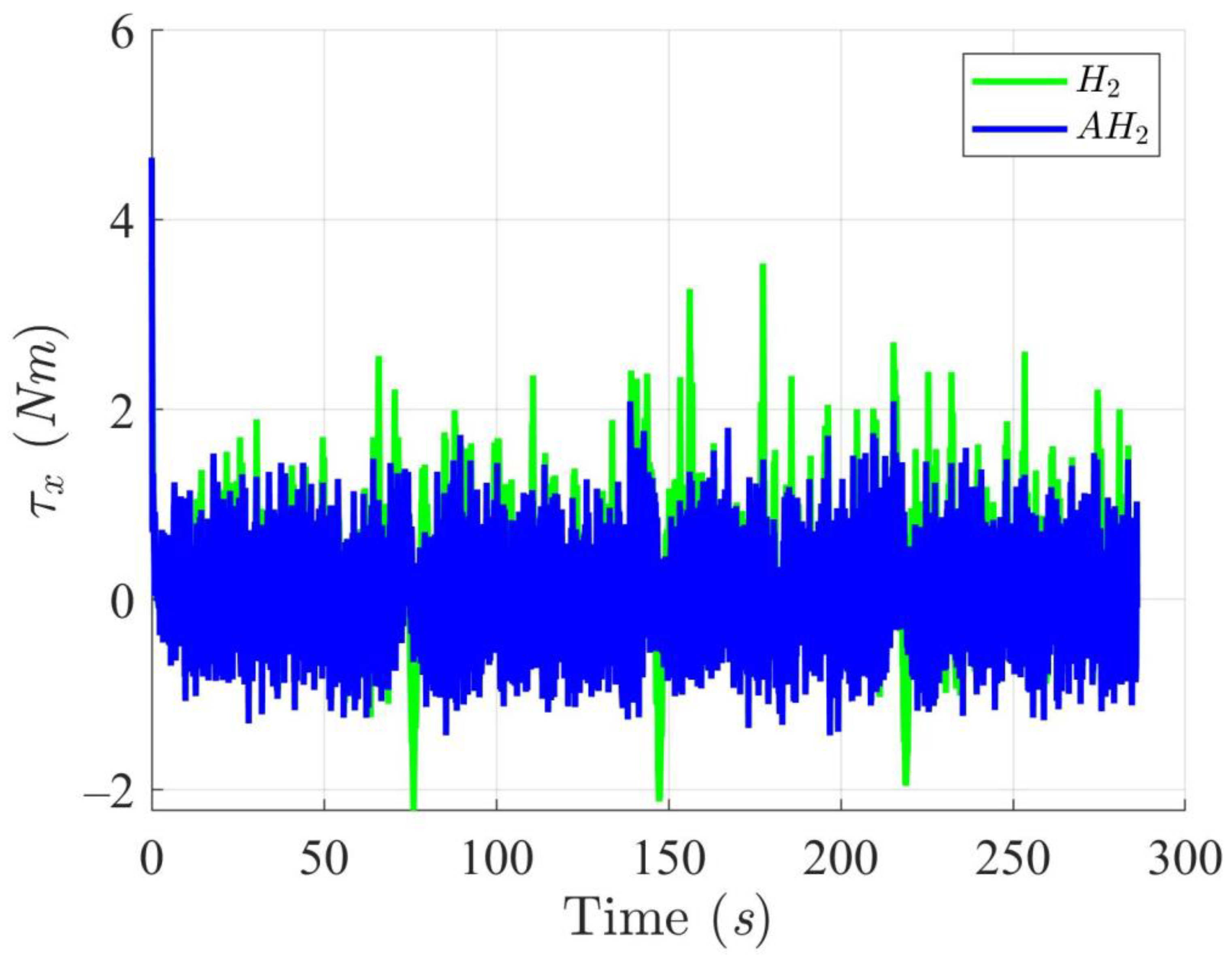
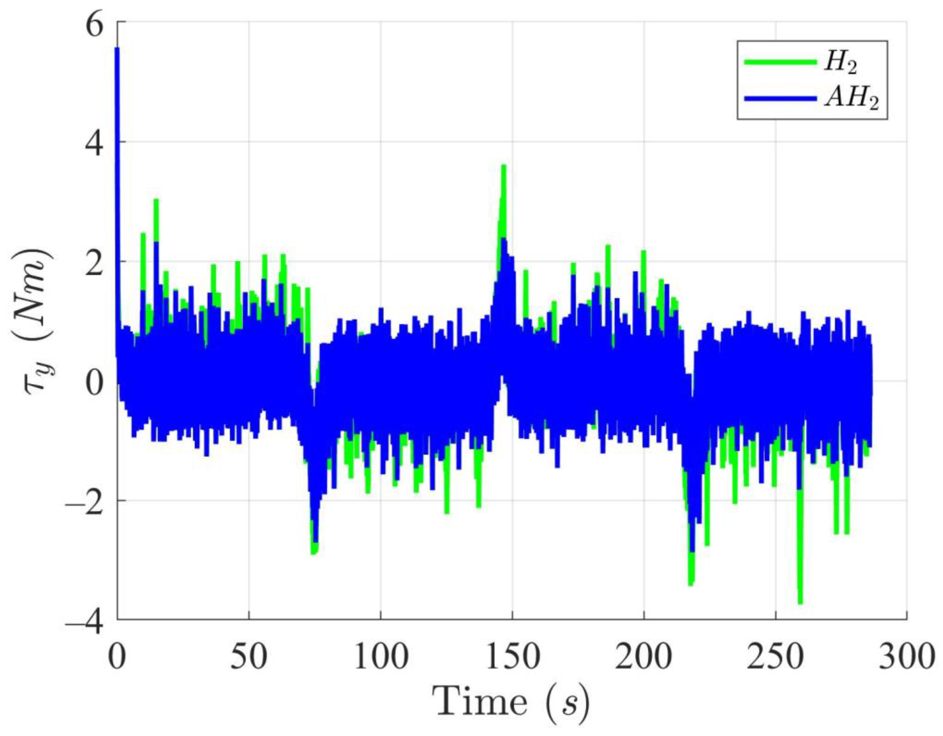
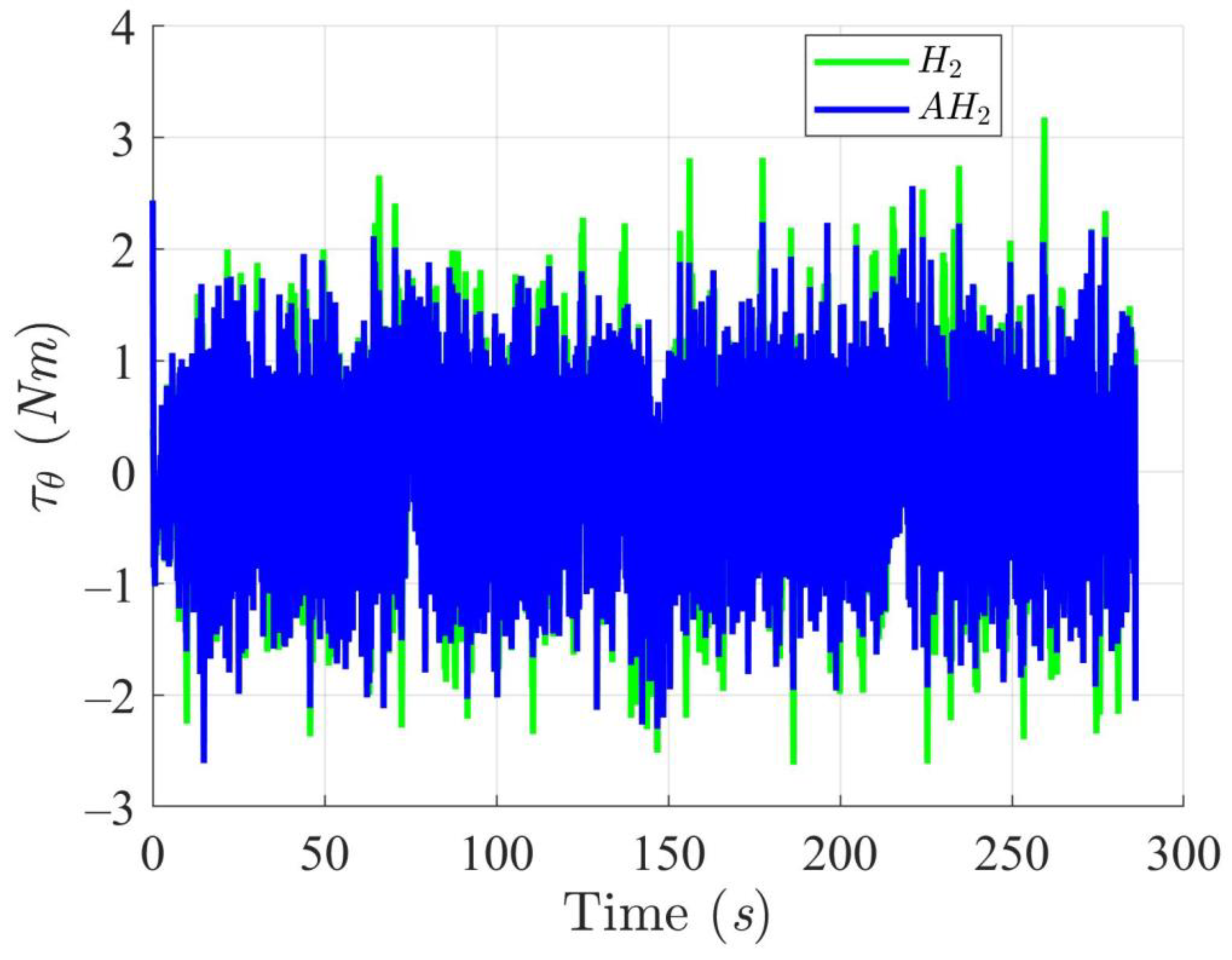
Figure 12, Figure 13, Figure 14 and Figure 15 display the trajectory and pose tracking performance of the DT under limited modeling uncertainties using both the H2 and adaptive H2 control methods. Figure 16, Figure 17 and Figure 18 detail the tracking errors in the XY plane, along with heading angle errors associated with these methods. The analysis indicates that the H2 control method has higher tracking errors, while the adaptive H2 control method achieves lower, acceptable errors. The results demonstrate that the adaptive H2 control method is more robust to modeling uncertainties, achieving greater accuracy in trajectory tracking. In Figure 12, Figure 15 and Figure 18, the heading angle of the WMR controlled by the H2 method exhibits noticeable fluctuations, especially at sharp turning points, highlighting the H2 method’s limitations in effectively guiding the WMR along the DT amid uncertainties. In contrast, the adaptive H2 control method closely follows the DT path. Furthermore, the control torques shown in Figure 19, Figure 20 and Figure 21 illustrate that the adaptive H2 control method requires less torque compared to the H2 method. These findings indicate that the adaptive H2 control method not only quickly aligns the WMR with the desired heading but also optimally generates control torque to maintain precise heading during trajectory tracking, thereby improving energy efficiency. In summary, the simulation results confirm that the adaptive H2 control method surpasses the H2 control method in both trajectory and pose tracking performance for the WMR in this scenario. Notably, the adaptive H2 method produces control outputs similar to those of the H2 method, delivering superior accuracy in trajectory tracking.

Figure 12.
Trajectory tracking of DT and orientation of the controlled WMR using H2 and adaptive H2 (AH2) methods for scenario 2.
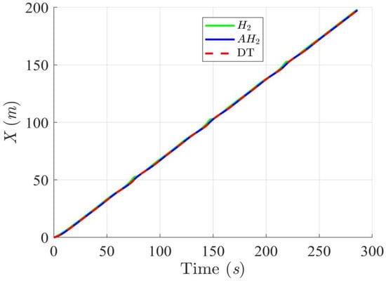
Figure 13.
Trajectory tracking results of the DT along the X-axis using H2 and adaptive H2 (AH2) methods for scenario 2.
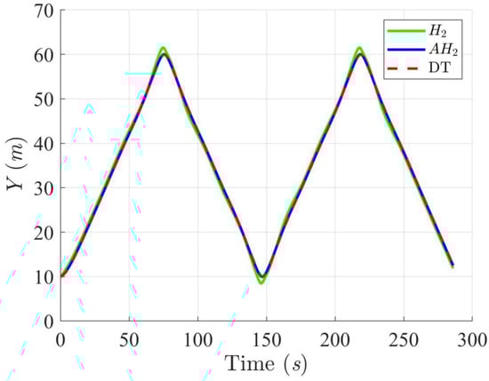
Figure 14.
Trajectory tracking results of the DT along the Y-axis using H2 and adaptive H2 (AH2) methods for scenario 2.

Figure 15.
Trajectory tracking results of the DT at an angle using H2 and adaptive H2 (AH2) methods for scenario 2.
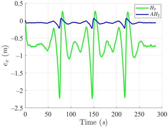
Figure 16.
Trajectory tracking errors along the X-axis utilizing the H2 and adaptive H2 (AH2) methods for scenario 2.

Figure 17.
Trajectory tracking errors along the Y-axis utilizing the H2 and adaptive H2 (AH2) methods for scenario 2.

Figure 18.
Trajectory tracking errors of heading angle utilizing the H2 and adaptive H2 (AH2) methods for scenario 2.

Figure 19.
Trajectory tracking torques along the X-axis utilizing the H2 and adaptive H2 (AH2) methods for scenario 2.

Figure 20.
Trajectory tracking torques along the Y-axis utilizing the H2 and adaptive H2 (AH2) methods for scenario 2.

Figure 21.
Trajectory tracking torques on heading angle utilizing the H2 and adaptive H2 (AH2) methods for scenario 2.
5. Experiments
Building on the derivation of the nonlinear adaptive optimal control design presented in Section 3, a practical controller is derived, as shown in Equation (49), which can be effectively implemented in the WMR control system using control chips. This section is organized into four key components: WMR hardware configurations, WMR integration operations, WMR verification process, and WMR tracking results.
5.1. WMR Hardware Configurations
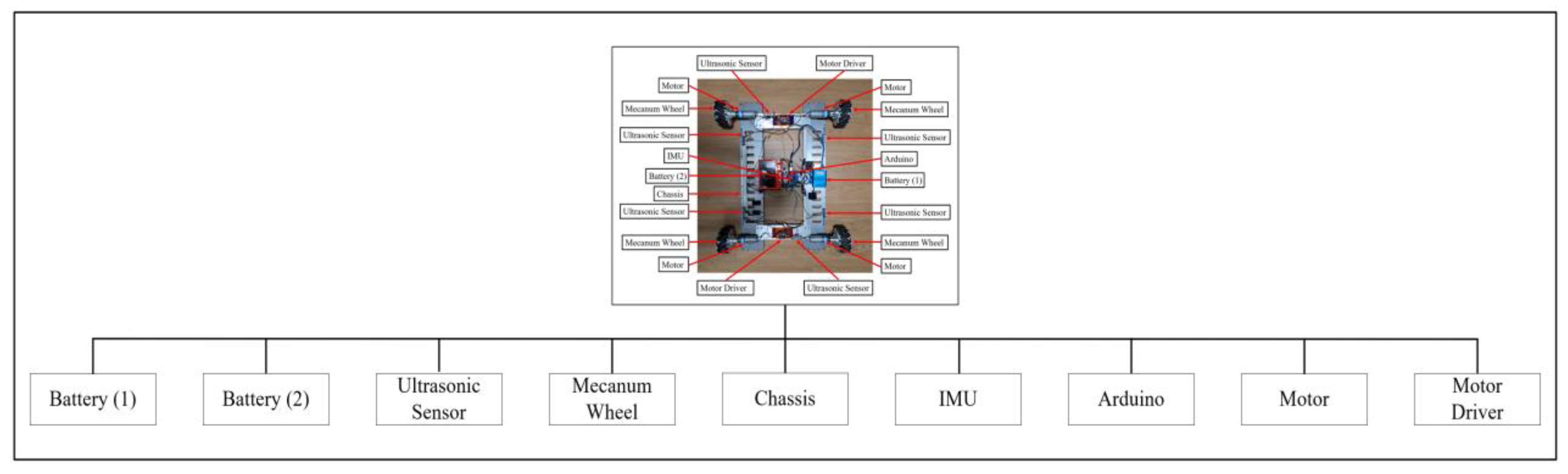
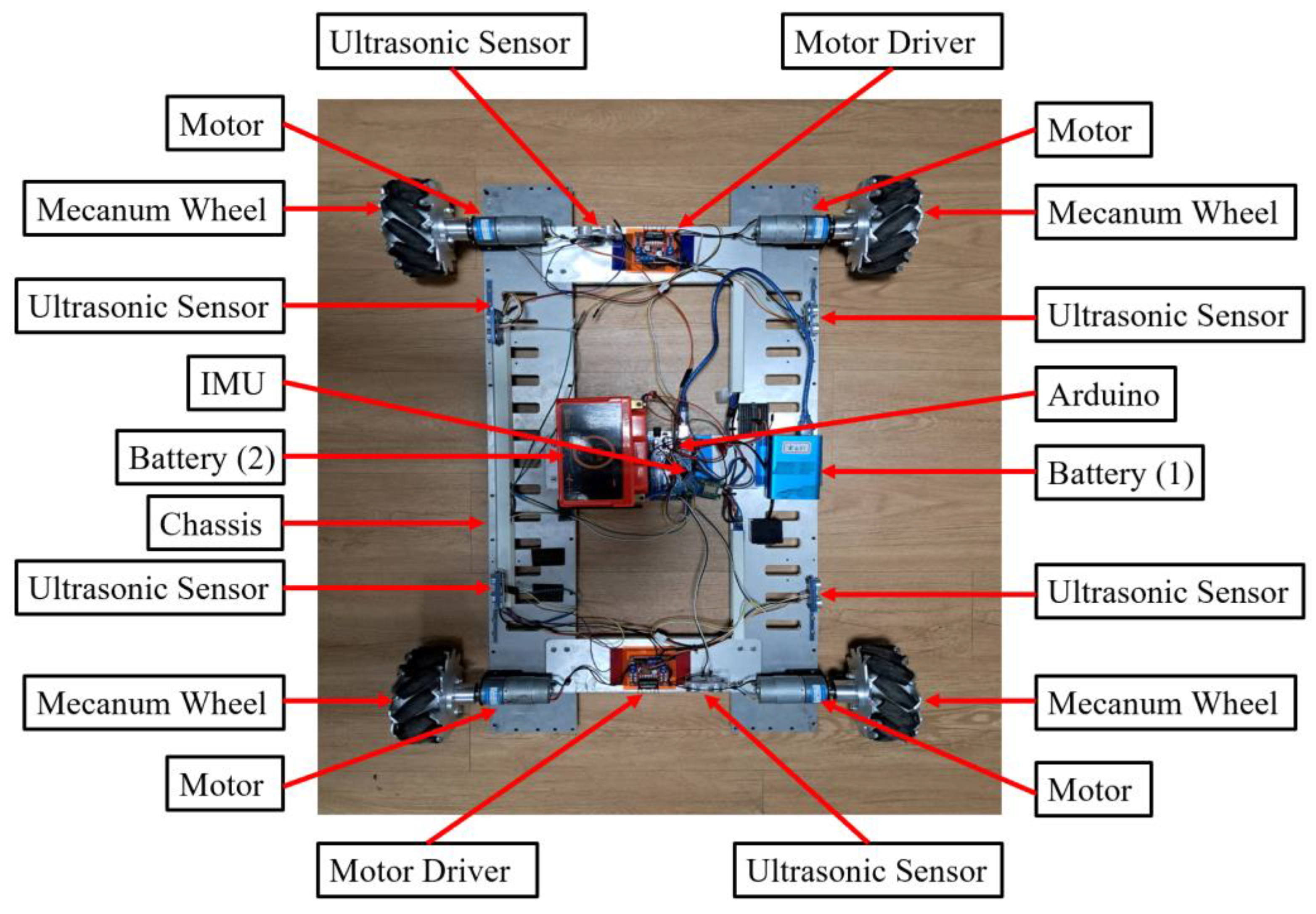
Figure 22 illustrates the overall hardware architecture of the WMR developed for this study. The architecture is divided into nine components: battery (1), battery (2), ultrasonic sensor, mecanum wheel, chassis, inertial measurement unit (IMU), Arduino, motor, and motor driver. Details regarding the electronic units used, their volumes, and attributes can be found in Table 6. Additionally, the WMR developed for experimental purposes is shown in Figure 23.
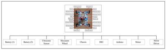
Figure 22.
The overall hardware architecture of the WMR.
Table 6.
The hardware configurations of the WMR [39].
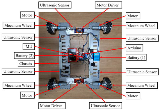
Figure 23.
The overall view of the WMR.
5.2. WMR Integration Operations
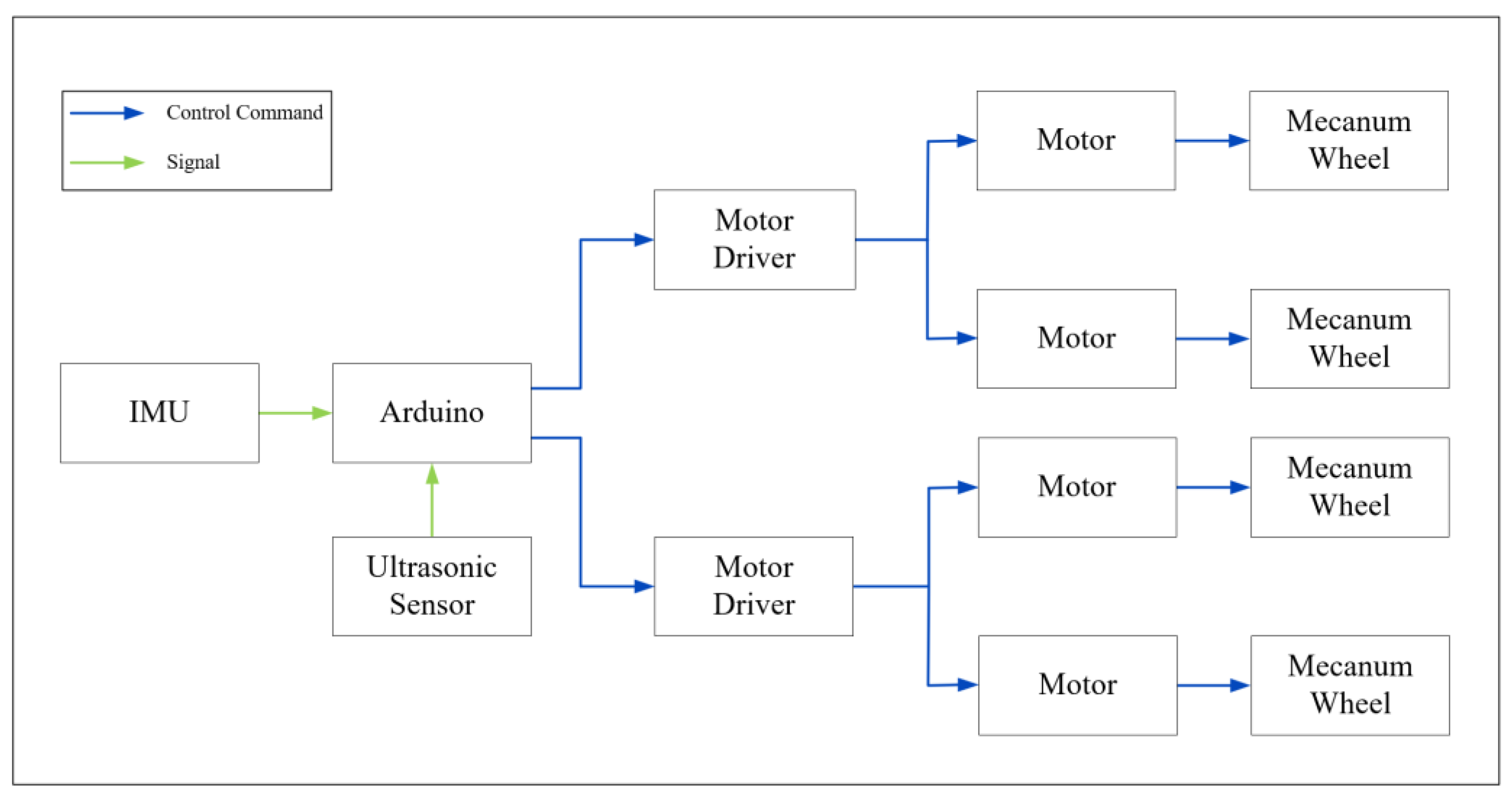
The connection diagram of the various electronic components of the WMR is shown in Figure 24. This diagram includes an inertial measurement unit (IMU), an Arduino, six ultrasonic sensors, two motor drivers, four motors, and four mecanum wheels, along with annotations for control commands and signals. Among these electronic components, the Arduino is the most critical, serving as the control core of the WMR. In addition to implementing the controller derived in this study, the Arduino also handles: 1. Receiving pose information from the IMU, 2. Receiving information from the ultrasonic sensors regarding the detection of boundary-colored boards and transmitting this information to the Arduino for optimal path navigation planning, and 3. Sending control commands calculated by the Arduino controller to the motor drivers to rotate the four mecanum wheels via the four motors.
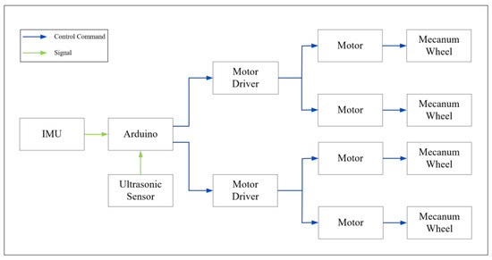
Figure 24.
The connection diagram of the various electronic components of the WMR.
The operational details of each electronic component are described as follows. Initially, the WMR will perform trajectory tracking according to the specified path and range. During the trajectory tracking process, if a boundary-colored board is encountered, the ultrasonic sensors will transmit information about the effective distance to the Arduino for obstacle avoidance and path re-planning. Furthermore, the ultrasonic sensors will continuously assess for boundary detection; if a boundary is detected, the Arduino will send control signals to the four motors to steer the mecanum wheels, preventing the WMR from exceeding the defined range. During the trajectory tracking task, the IMU will continuously transmit real-time pose data to the Arduino, enabling dynamic adjustments to the control commands for optimal path planning. This process will remain active throughout the entire trajectory tracking operation until the mission is concluded.
5.3. WMR Verification Process
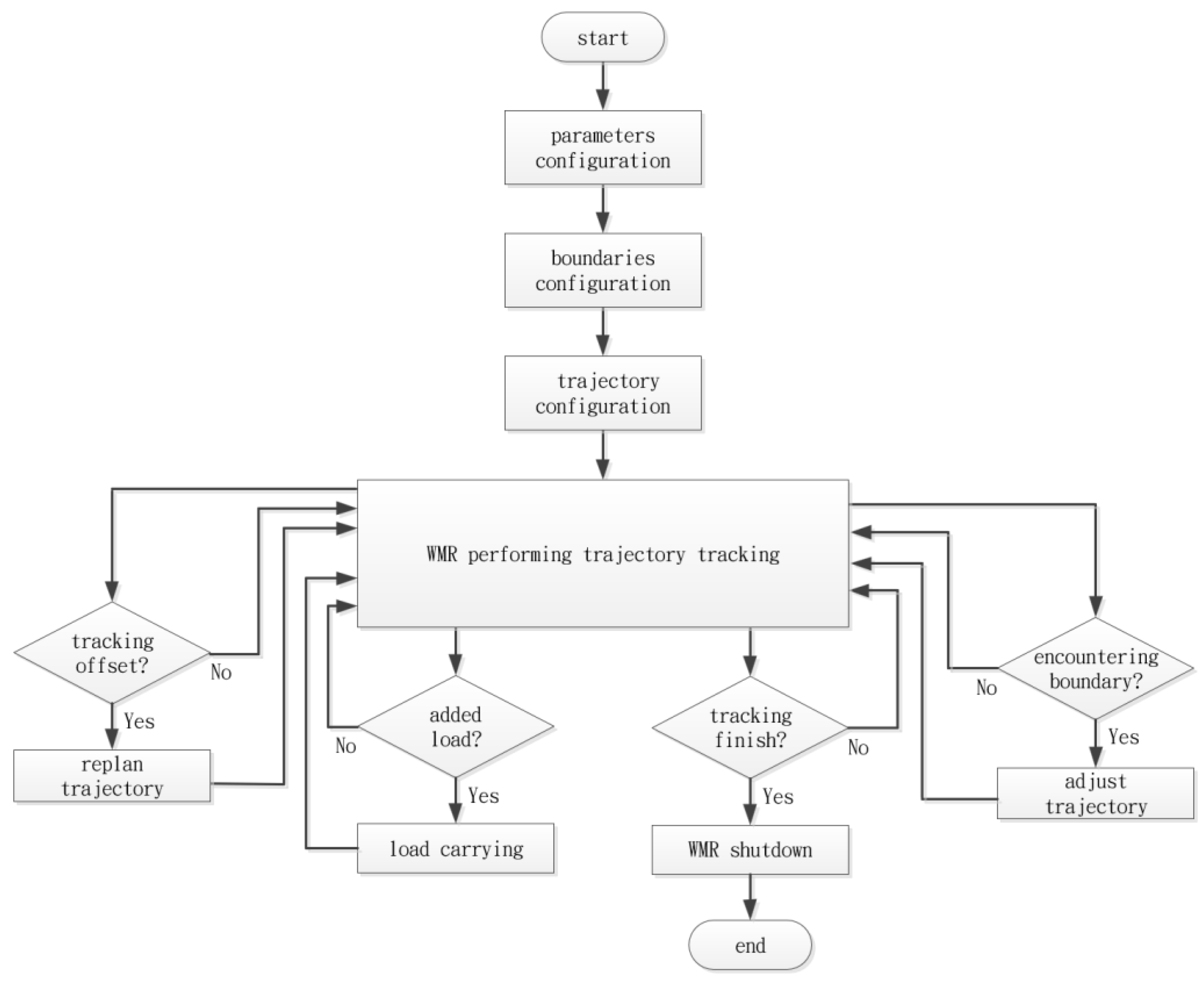
Figure 25 illustrates the flowchart for the WMR trajectory tracking process. First, the relevant parameters for the WMR are set, followed by the establishment of the boundary range for trajectory tracking, and finally, the definition of the DT for the WMR to follow. Subsequently, the task of tracking the DT is executed according to the established range and path. During the trajectory tracking process, the ultrasonic sensors continuously monitor for boundary detection. If a boundary is encountered, the Arduino control board will execute a steering action (adjust trajectory) to prevent exceeding the defined boundary limits. Moreover, a random load will be applied to the WMR throughout the trajectory tracking process, while the IMU continuously relays the current pose data to the Arduino for real-time control adjustments. If there is a deviation in the WMR’s pose, a path re-planning action (replan trajectory) will be executed to adjust the control commands for the four mecanum wheels, thereby optimizing the trajectory tracking and completing the tracking task.
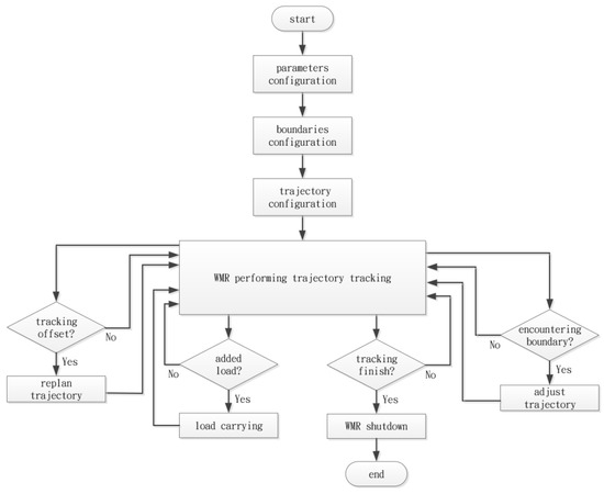
Figure 25.
The flowchart of the WMR verification process.
5.4. WMR Tracking Results
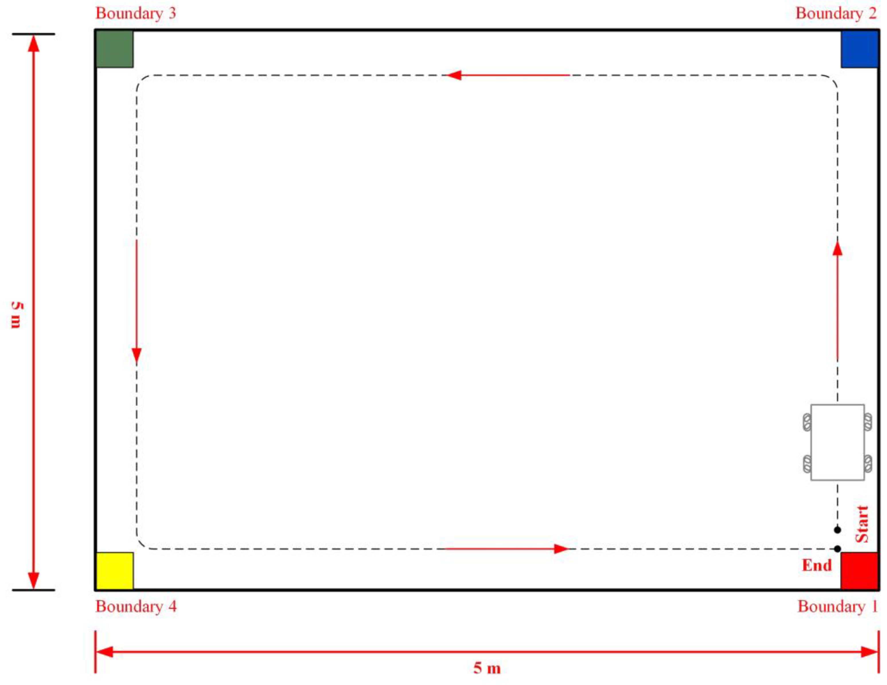
Figure 26 illustrates the trajectory tracking of the WMR along the DT. The DT, measuring 5 m in length and 5 m in width, is enclosed by boundaries formed with four distinct colors: red (Boundary 1), blue (Boundary 2), green (Boundary 3), and yellow (Boundary 4). Once the WMR configures the relevant parameters and positions itself at the starting point (Start), it initiates the trajectory tracking task following the direction indicated by the red arrow. The trajectory tracking process concludes at the stopping point (End) upon the successful completion of the task. During the trajectory tracking process, if the WMR encounters a boundary, it will adjust its trajectory accordingly to ensure continuous tracking of the desired trajectory.
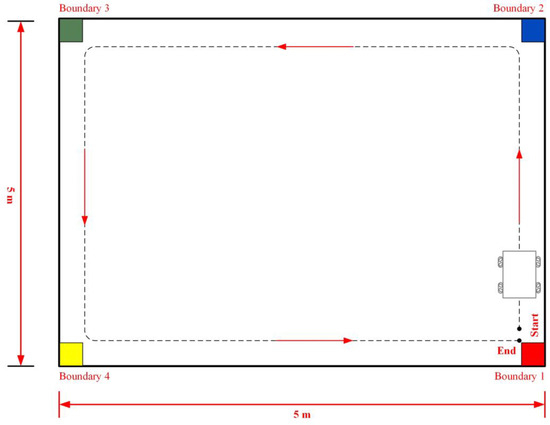
Figure 26.
Schematic representation of the WMR’s trajectory tracking compared to the DT.
Based on the schematic diagram in Figure 26, an experimental trajectory tracking field for the WMR was constructed on the third floor of the Department of Mechanical Engineering at National Pingtung University of Science and Technology, as shown in Figure 27. The field measures 5 m in length and 5 m in width, surrounded by boundary boards in four distinct colors: red (Boundary 1), blue (Boundary 2), green (Boundary 3), and yellow (Boundary 4). The WMR begins its trajectory tracking task from the starting point (Start) following the direction indicated by the red arrow. Upon completing the trajectory tracking task, the WMR ultimately stops at the stopping point (End).
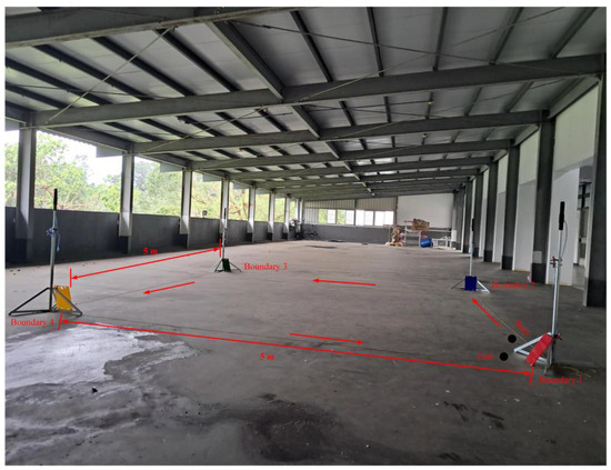
Figure 27.
Experimental setup for the real-world trajectory tracking of the WMR.
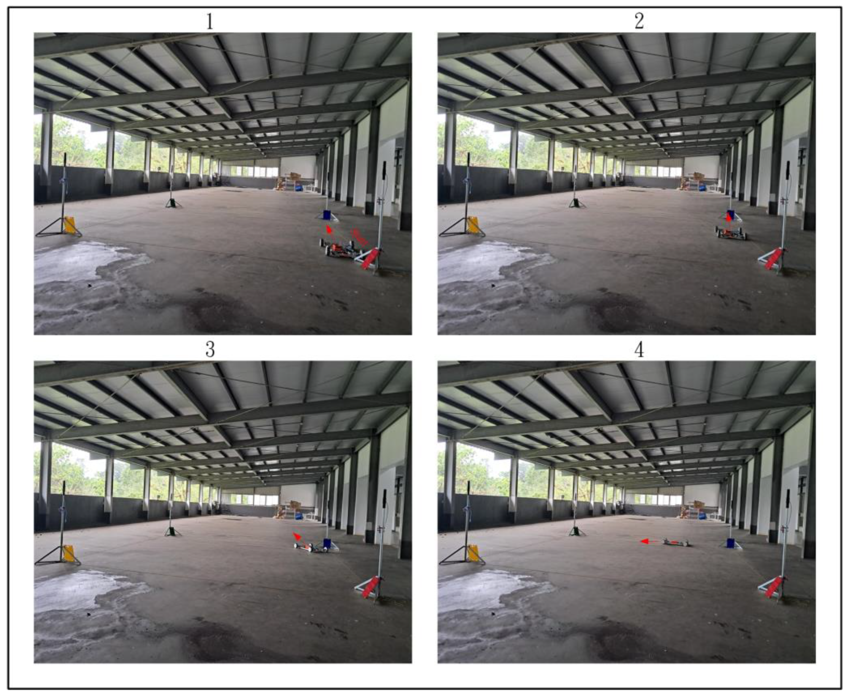
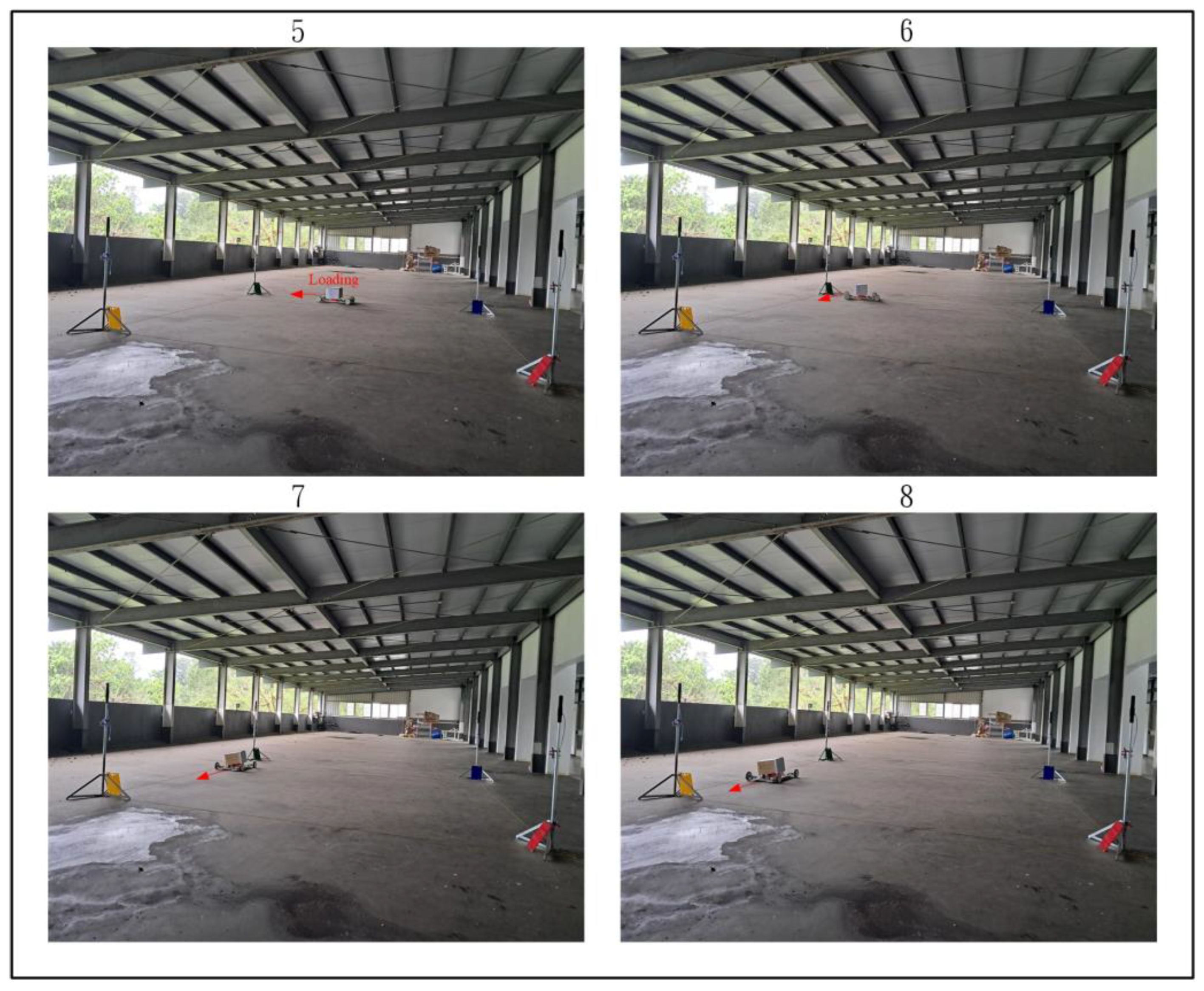
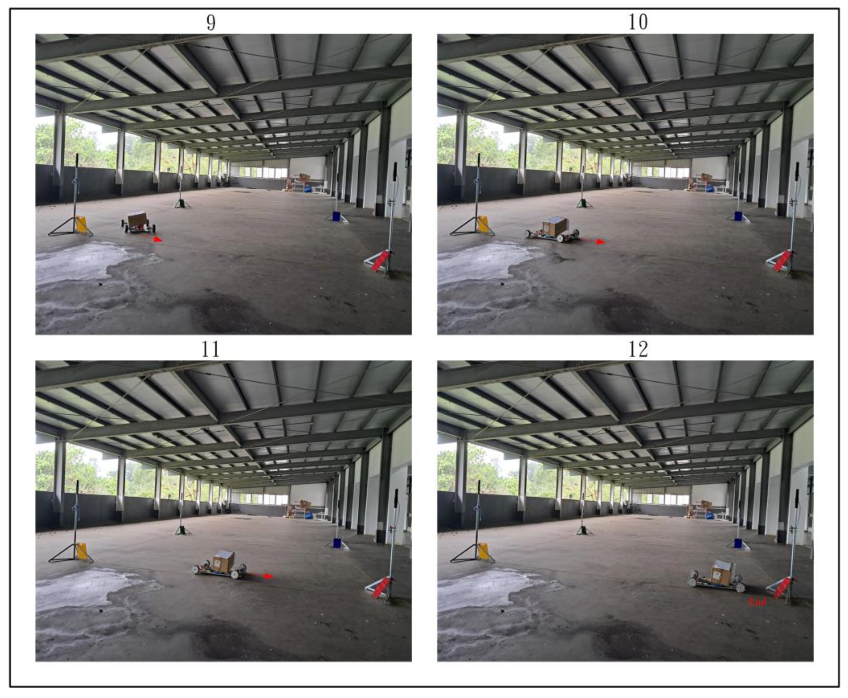
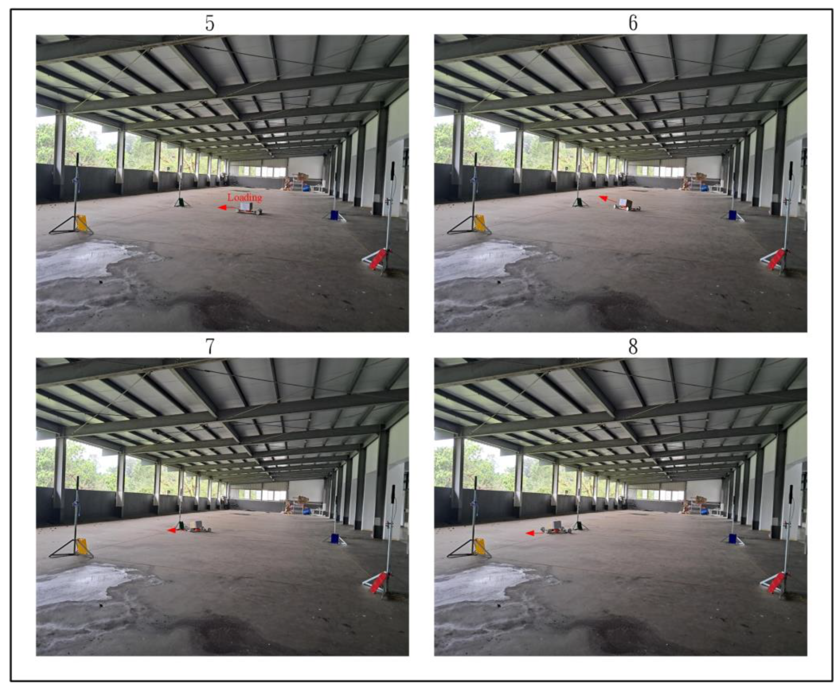
Figure 28, Figure 29 and Figure 30 demonstrate the trajectory tracking performance of the WMR under the adaptive H2 control method. In Figure 28(1), the WMR starts from the designated starting point (Start) without any additional load and begins its trajectory tracking task in the direction indicated by the red arrow. Figure 28(2–4) show the WMR progressing along the DT, enclosed by boundary boards, without deviating from the designated path. In Figure 29(5), the WMR is loaded with an additional 3-kg weight. Despite this load, the WMR continues to follow the DT accurately without exceeding the path or crossing the boundary boards, as illustrated in Figure 29(6–8) and Figure 30(9–11). Upon completing the trajectory tracking task, the WMR stops precisely at the designated endpoint (End), as shown in Figure 30(12).
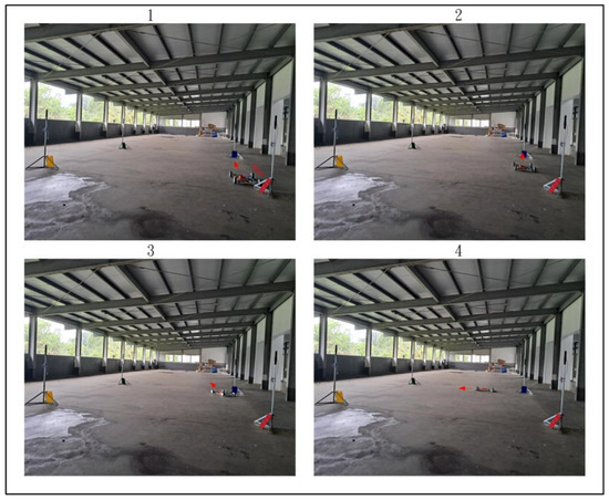
Figure 28.
Actual trajectory tracking of the WMR using the adaptive H2 control method under unloaded conditions.
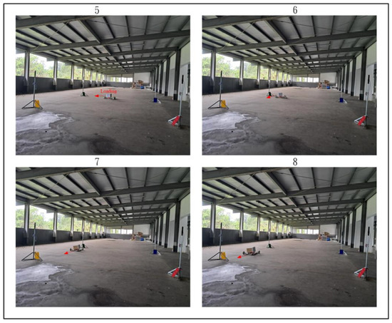
Figure 29.
Actual trajectory tracking of the WMR using the adaptive H2 control method under loaded conditions.
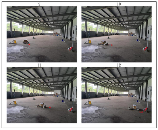
Figure 30.
Completion of the actual trajectory tracking task of the WMR using the adaptive H2 control method.
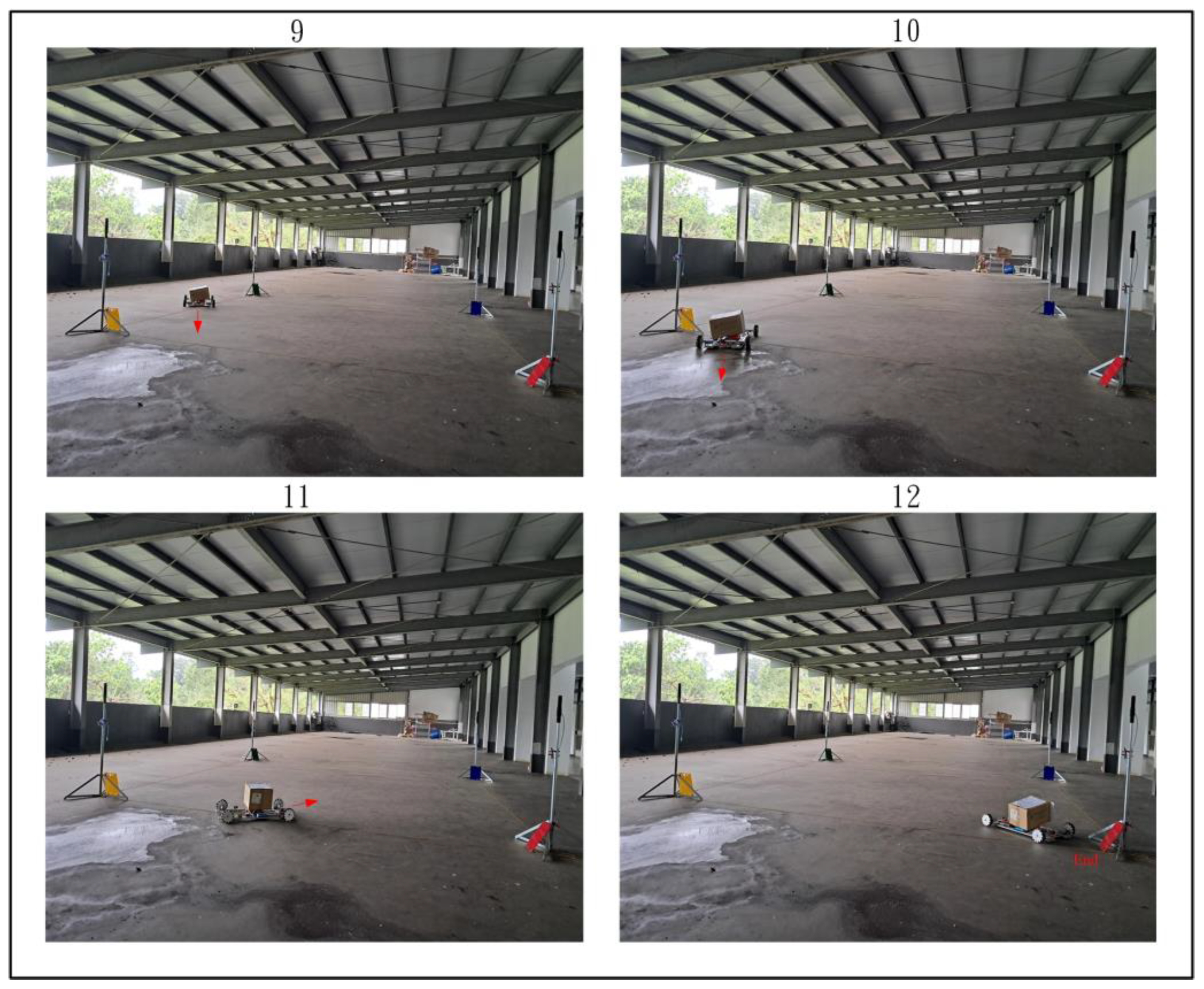
Under identical experimental conditions, the H2 control method was also applied for trajectory tracking, with the results shown in Figure 31, Figure 32 and Figure 33. In Figure 31(1), the WMR starts from the designated starting point (Start) without any additional load and begins its trajectory tracking task in the direction indicated by the red arrow. Figure 31(2–4) illustrate the WMR progressing along the DT enclosed by boundary boards, but with slight deviations from the designated path. In Figure 32(5), the WMR is loaded with an additional 3-kg weight. After applying this load, the WMR exhibits drifting behavior, causing it to deviate from the desired trajectory and cross the boundary boards during both forward and turning movements, as depicted in Figure 32(6–8) and Figure 33(9–11). Furthermore, upon completing the trajectory tracking task, the WMR fails to stop at the designated endpoint (End), as shown in Figure 33(12).
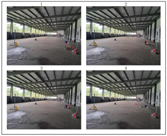
Figure 31.
Actual trajectory tracking of the WMR using the H2 control method under unloaded conditions.
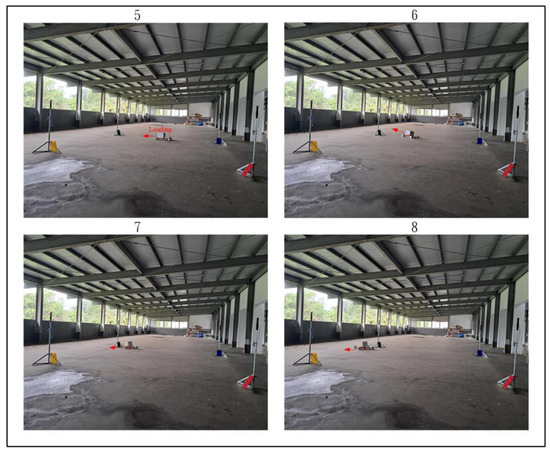
Figure 32.
Actual trajectory tracking of the WMR using the H2 control method under loaded conditions.

Figure 33.
Completion of the actual trajectory tracking task of the WMR using the H2 control method.
A comparison of the trajectory tracking performance between the two control methods reveals that the adaptive H2 control method enables the WMR to accurately follow the designated trajectory and successfully complete the tracking task even when a 3-kg load is applied. In contrast, the H2 control method demonstrates significantly poorer tracking performance, particularly when the WMR is subjected to the additional load, resulting in pronounced positional and orientation deviations during both straight-line and turning movements. These experimental results validate the effectiveness of the proposed adaptive H2 control method in overcoming and mitigating the effects of model uncertainties.
6. Conclusions
This study presents an adaptive H2 control method to address the trajectory tracking problem of WMR under model uncertainties, demonstrating ease of implementation and excellent energy-saving performance. The proposed method also validates the robustness of the WMR trajectory tracking system when subjected to these uncertainties. To evaluate the performance of the proposed adaptive H2 control method, two comparative simulations were performed against the H2 control method, using a 100 m × 30 m rectangular trajectory and a double triangle trajectory with a base length of 200 m as the DTs for WMR trajectory tracking. The simulation results, with 20% model uncertainty, show that the adaptive H2 control method significantly outperforms the H2 control method in control response, trajectory tracking precision, adaptability to model uncertainties, and energy efficiency. The adaptive H2 control method demonstrated exceptional performance in tracking the rectangular trajectory and the double triangle trajectory, effectively handling the nonlinear dynamics and uncertainties inherent in WMR.
Furthermore, both the adaptive H2 and H2 control methods were implemented on an actual WMR system, using a simple Arduino control board and other auxiliary electronic components to achieve real-world trajectory tracking. The experimental results indicate that under conditions with a 3 kg load and within the specified operational area, the adaptive H2 control method successfully completed the trajectory tracking task without exceeding the DT and boundary, while maintaining smooth performance. In contrast, under the same experimental conditions, the H2 control method not only exceeded the DT and boundary but also failed to complete the trajectory tracking task smoothly. Therefore, both the simulations and experimental results demonstrate that the proposed adaptive H2 control method outperforms the H2 method in terms of control performance.
Funding
This research received no external funding.
Data Availability Statement
All data revealed in this paper are generated during the study.
Conflicts of Interest
The author declares no conflicts of interest.
Appendix A
The performance criterion presented in Equation (27) can be expressed in the following form:
Using the terminal condition , the subsequent outcome can be deduced:
Substituting the trajectory tracking error dynamics from Equation (25) into (A2) yields the following result:
Consequently, by applying the , along with the adaptive law from Equation (31) and the differential in Equation (28), the following is derived:
By choosing the control law as defined in Equation (30), Equation (A4) can be concisely reduced to the following form:
This corresponds to Equation (27), thus completing the proof.
References
- Maddahi, Y.; Maddahi, A.; Monsef, S. Design Improvement of Wheeled Mobile Robots: Theory and Experiment. World Appl. Sci. J. 2012, 16, 263–274. [Google Scholar]
- Demetris, S.; Demetrios, G.E.; Christos, G.P.; Marios, M.P. Fault Detection for Service Mobile Robots Using Model-Based Method. Auton. Robot. 2016, 40, 383–394. [Google Scholar]
- Gao, X.; Li, J.; Fan, L.; Zhou, Q.; Yin, K.; Wang, J.; Song, C.; Huang, L.; Wang, Z. Review of Wheeled Mobile Robots’ Navigation Problems and Application Prospects in Agriculture. IEEE Access 2018, 6, 49248–49268. [Google Scholar] [CrossRef]
- Mishra, S.; Sharma, M.; Mohan, S.B. Fault Tolerant Control of an Omni Directional Mobile Robot with Four Mecanum Wheels. Def. Sci. J. 2019, 69, 353–360. [Google Scholar] [CrossRef]
- Rubio, F.; Valero, F.; Llopis-Albert, C. A Review of Mobile Robots: Concepts, Methods, Theoretical Framework, and Applications. Int. J. Adv. Robot. Syst. 2019, 16, 172988141983959. [Google Scholar] [CrossRef]
- Luigi, T.; Giovanni, C.; Andrea, B.; Paride, C.; Lorenzo, B.; Giuseppe, Q. Wheeled Mobile Robots: State of the Art Overview and Kinematic Comparison Among Three Omnidirectional Locomotion Strategies. J. Intell. Robot. Syst. 2022, 106, 57. [Google Scholar]
- Luis, M.C.; Andrés, S.M.R.; Francisco, R.; Vicente, F.B. Advanced Motor Control for Improving the Trajectory Tracking Accuracy of a Low-Cost Mobile Robot. Machines 2023, 11, 14. [Google Scholar]
- Nitin, S.; Jitendra, K.P.; Surajit, M. A Review of Mobile Robots: Applications and Future Prospect. Int. J. Precis. Eng. Manuf. 2023, 24, 1695–1706. [Google Scholar]
- Zhang, C.; Cen, C.; Huang, J. An Overview of Model-Free Adaptive Control for the Wheeled Mobile Robot. World Electr. Veh. J. 2024, 15, 396. [Google Scholar] [CrossRef]
- Linjie, X.; Qinglin, W.; Jinhua, S.; Yuan, L. Robust Adaptive Tracking Control of Wheeled Mobile Robot. Robot. Auton. Syst. 2016, 78, 36–48. [Google Scholar]
- Xie, H.; Zheng, J.; Sun, Z.; Wang, H.; Chai, R. Finite-time Tracking Control for Nonholonomic Wheeled Mobile Robot Using Adaptive Fast Nonsingular Terminal Sliding Mode. Nonlinear Dyn. 2022, 110, 1437–1453. [Google Scholar] [CrossRef]
- Bong, S.P.; Sung, J.Y.; Jin, B.P.; Yoon, H.C. A Simple Adaptive Control Approach for Trajectory Tracking of Electrically Driven Nonholonomic Mobile Robots. IEEE Trans. Control Syst. Technol. 2010, 18, 1199–1206. [Google Scholar]
- Sameh, F.H.; Hassan, M.A. Modeling and Control of Wheeled Mobile Robot with Four Mecanum Wheels. Eng. Technol. J. 2021, 39, 779–789. [Google Scholar]
- Swati, M.; Santhakumar, M.; Santosh, K.V. Performance Investigations of an Improved Backstepping Operational-space Position Tracking Control of a Mobile Manipulator. Def. Sci. J. 2021, 71, 436–447. [Google Scholar]
- Jiang, M.; Chen, L.; Wang, Y.; Wu, H. Adaptive Backstepping Control for Mecanum-Wheeled Omnidirectional Vehicle Using Neural Networks. IEEJ Trans. Electr. Electron. Eng. 2022, 17, 378–386. [Google Scholar] [CrossRef]
- Umar, Z.; Salinda, B.; Mohamad, S.Z.A.; Mohd, S.A.M.; Hameedah, S.H. Nonlinear PID Controller for Trajectory Tracking of a Differential Drive Mobile Robot. J. Mech. Eng. Res. Dev. 2020, 43, 255–270. [Google Scholar]
- Nguyen, H.T.; Trinh, T.K.L.; Hoang, T.; Le, Q.D. Trajectory Tracking Control for Differential-Drive Mobile Robot by a Variable Parameter PID Controller. Int. J. Mech. Eng. Robot. Res. 2022, 11, 614–621. [Google Scholar]
- Nguyen, H.T.; Trinh, T.K.L.; Le, Q.D. Trajectory Tracking Control for Mecanum Wheel Mobile Robot by Time-Varying Parameter PID Controller. Bull. Electr. Eng. Inform. 2022, 11, 1902–1910. [Google Scholar]
- Rasha, M.H. Design a New Hybrid Controller Based on an Improvement Version of Grey Wolf Optimization for Trajectory Tracking of Wheeled Mobile Robot. FME Trans. 2023, 51, 140–148. [Google Scholar]
- Muhamad, A.; Riky, D.P. Mecanum 4 Omni Wheel Directional Robot Design System Using PID Method. J. Fuzzy Syst. Control. 2023, 1, 6–13. [Google Scholar]
- Veer, A.; Shital, S.C. Adaptive Robust Control of Mecanum-wheeled Mobile Robot with Uncertainties. Nonlinear Dyn. 2017, 87, 2147–2169. [Google Scholar]
- Wang, G.; Zhou, C.; Yu, Y.; Liu, X. Adaptive Sliding Mode Trajectory Tracking Control for WMR Considering Skidding and Slipping via Extended State Observer. Energies 2019, 12, 3305. [Google Scholar] [CrossRef]
- Yuan, Z.; Tian, Y.; Yin, Y.; Wang, S.; Liu, J.; Wu, L. Trajectory Tracking Control of a Four Mecanum Wheeled Mobile Platform: An Extended State Observer-Based Sliding Mode Approach. IET Control. Theory Appl. 2020, 14, 415–426. [Google Scholar] [CrossRef]
- Rishabh, D.Y.; Viswa, N.S. Adaptive Sliding Mode Control for Autonomous Vehicle Platoon under Unknown Friction Forces. In Proceedings of the Conference: 2021 20th International Conference on Advanced Robotics (ICAR), Ljubljana, Slovenia, 6–10 December 2021. [Google Scholar]
- Pankaj, S.Y.; Vandana, A.; Mohanta, J.; Ahmed, M.D.F. A Robust Sliding Mode Control of Mecanum Wheel-Chair for Trajectory Tracking. Mater. Today Proc. 2022, 56, 623–630. [Google Scholar]
- Javad, M.; Akbar, S.; Reza, A.T. Design of Fixed-Time Terminal Sliding Mode Control for Robot with Mecanum Wheels. J. Nonlinear Syst. Electr. Eng. 2022, 8, 19–37. [Google Scholar]
- Pham, A.T.; Nguyen, M.L. Trajectory Tracking Control of Omnidirectional Mobile Robots: A Model-Free Control-Based Approach. J. Appl. Sci. Eng. 2023, 27, 3687–3696. [Google Scholar]
- Mohanty, P.K.; Parhi, D.R. A New Hybrid Intelligent Path Planner for Mobile Robot Navigation Based on Adaptive Neuro-Fuzzy Inference System. Aust. J. Mech. Eng. 2015, 13, 195–207. [Google Scholar] [CrossRef]
- Dong, N.M.; Hiep, D.Q.; Nam, D.P.; Tien, N.M.; Duy, N.B. An Adaptive Fuzzy Dynamic Surface Control Tracking Algorithm for Mecanum Wheeled Mobile Robot. Int. J. Mech. Eng. Robot. Res. 2023, 12, 354–361. [Google Scholar]
- Chen, Y.-H.; Chen, Y.-Y. Nonlinear Adaptive Fuzzy Control Design for Wheeled Mobile Robots with Using the Skew Symmetrical Property. Symmetry 2023, 15, 221. [Google Scholar] [CrossRef]
- Zenon, H. Robust Neural Networks Control of Omni-Mecanum Wheeled Robot with Hamilton-Jacobi Inequality. J. Theor. Appl. Mech. 2018, 56, 1193–1204. [Google Scholar]
- Mateusz, S.; Marcin, S. Neural Tracking Control of a Four-Wheeled Mobile Robot with Mecanum Wheels. Appl. Sci. 2022, 12, 5322. [Google Scholar] [CrossRef]
- Ma, C.; Li, X.; Xing, G.; Dian, S. A T-S Fuzzy Quaternion-Value Neural Network-Based Data-Driven Generalized Predictive Control Scheme for Mecanum Mobile Robot. Processes 2022, 10, 1964. [Google Scholar] [CrossRef]
- Trinh, T.K.L.; Nguyen, T.T.; Hoang, T.; Thai, N. A Neural Network Controller Design for the Mecanum Wheel Mobile Robot. Eng. Technol. Appl. Sci. Res. 2023, 13, 10541–10547. [Google Scholar]
- Chen, Y.-H.; Li, T.H.S.; Chen, Y.-Y. A Novel Nonlinear Control Law with Trajectory Tracking Capability for Mobile Robots: Closed-Form Solution Design. Appl. Math. Inf. Sci. 2013, 7, 749–754. [Google Scholar] [CrossRef]
- Chen, Y.-H.; Lou, S.-J. Control Design of a Swarm of Intelligent Robots: A Closed-Form H2 Nonlinear Control Approach. Appl. Sci. 2020, 10, 1055. [Google Scholar] [CrossRef]
- Samia, M.; Guillaume, G.; El-Mostafa, E.; Mustapha, O.; Alain, P. Trajectory Tracking and Time Delay Management of Four-Mecanum Wheeled Mobile Robots (4-MWMR). In Proceedings of the 15th European Workshop on Advanced Control and Diagnosis (ACD 2019), Bologna, Italy, 21–22 November 2019. [Google Scholar]
- Matthew, T.W.; Daniel, T.G.; Tony, J.P. Collinear Mecanum Drive: Modeling, Analysis, Partial Feedback Linearization, and Nonlinear Control. IEEE Trans. Robot. 2021, 37, 642–658. [Google Scholar]
- Chen, Y.-H. Control Design and Implementation of Autonomous Robotic Lawnmower. Mathematics 2024, 12, 3324. [Google Scholar] [CrossRef]
- Chen, Y.-H.; Chen, Y.-Y. Trajectory Tracking Design for A Swarm of Autonomous Mobile Robots: A Nonlinear Adaptive Optimal Approach. Mathematics 2022, 10, 3901. [Google Scholar] [CrossRef]
- Sameh, F.H.; Hassan, M.A. Design of Hybrid Controller for the Trajectory Tracking of Wheeled Mobile Robot with Mecanum Wheels. J. Mech. Eng. Res. Dev. 2020, 43, 400–414. [Google Scholar]


Disclaimer/Publisher’s Note: The statements, opinions and data contained in all publications are solely those of the individual author(s) and contributor(s) and not of MDPI and/or the editor(s). MDPI and/or the editor(s) disclaim responsibility for any injury to people or property resulting from any ideas, methods, instructions or products referred to in the content. |
© 2024 by the author. Licensee MDPI, Basel, Switzerland. This article is an open access article distributed under the terms and conditions of the Creative Commons Attribution (CC BY) license (https://creativecommons.org/licenses/by/4.0/).