Analytical Solutions and Computer Modeling of a Boundary Value Problem for a Nonstationary System of Nernst–Planck–Poisson Equations in a Diffusion Layer

Abstract

This article proposes various new approximate analytical solutions of the boundary value problem for the non-stationary system of Nernst–Planck–Poisson (NPP) equations in the diffusion layer of an ideally selective ion-exchange membrane at overlimiting current densities. As is known, the diffusion layer in the general case consists of a space charge region and a region of local electroneutrality. The proposed analytical solutions of the boundary value problems for the non-stationary system of Nernst–Planck–Poisson equations are based on the derivation of a new singularly perturbed nonlinear partial differential equation for the potential in the space charge region (SCR). This equation can be reduced to a singularly perturbed inhomogeneous Burgers equation, which, by the Hopf–Cole transformation, is reduced to an inhomogeneous singularly perturbed linear equation of parabolic type. Inside the extended SCR, there is a sufficiently accurate analytical approximation to the solution of the original boundary value problem. The electroneutrality region has a curvilinear boundary with the SCR, and with an unknown boundary condition on it. The article proposes a solution to this problem. The new analytical solution methods developed in the article can be used to study non-stationary boundary value problems of salt ion transfer in membrane systems. The new analytical solution methods developed in the article can be used to study non-stationary boundary value problems of salt ion transport in membrane systems.

1. Introduction

Boundary value problems for the Nernst–Planck–Poisson (NPP) system of equations are used in modelling transfer in electrode and electromembrane systems (EMS) in diffusion layers, desalination channels, microfluidic devices, etc. [1,2,3,4,5,6,7]. Numerous works by Grafov B.M., Chernenko A.A. [8], Nikonenko V.V. [9,10], Rubinstein I., Zaltsman B. [11,12], Listovnichy A.V., Lebedev K.A. and others [13,14] are devoted to methods of analytical and numerical solution of these boundary value problems. Few works are devoted to non-stationary problems, which is explained by mathematical difficulties. Methods of exact or approximate analytical solutions of non-stationary boundary value problems have not been developed. At the same time, obtaining exact solutions is an important and urgent task, since it makes it possible to study the properties of the solution with exhaustive completeness.

At the same time, the study of non-stationary transfer of a binary electrolyte in a diffusion layer is interesting in that it allows one to determine the structure of the diffusion layer and its change over time, which is necessary, for example, for the asymptotic analysis of problems, the establishment of simple engineering calculation formulas for the dependence of the distribution of concentration, and the determination of electric field strength on the parameters of the problem. The studies of non-stationary problems are considered in [15,16]. In these works, main attention is paid to the over-limit potentiodynamic mode and the analysis of the settling time depending on the parameters of the problems. The works [16,17] consider “shock electrodialysis”—a recently developed method of water desalination in microscale pores near an ion-selective element, in which a deionization wave propagates through a microchannel or a porous medium with a sharp boundary between the concentrated and depleted zones. Deionization waves can be compared with a charge wave, since the deionization region actually coincides with the SCR. In contrast to “shock electrodialysis”, this work studies the depleted diffusion layer near the ion-exchange membrane, which has macroscale dimensions of the order of millimeters.

A number of works investigate the use of pulsed current modes [18,19,20,21,22,23,24,25,26,27] with currents of different duration and different shapes: rectangular, triangular, etc.

As is known, the diffusion layer in the general case consists of the SPL and the region of local electroneutrality [12]. The proposed article presents new analytical solutions of boundary value problems for a non-stationary system of equations of the NPP, based on the general idea of obtaining a singularly perturbed nonlinear differential equation with partial derivatives for the potential in the SCR. This equation is reduced to a singularly perturbed inhomogeneous Burgers equation, which, unlike the homogeneous Burgers equation, describes the dynamics of the system, with an “injection” of energy, which actually occurs in the diffusion layer when an external electric field is applied. By Hopf–Cole transformation, the singularly perturbed inhomogeneous Burgers equation is reduced to an inhomogeneous singularly perturbed linear equation of parabolic type. In the electroneutrality region (ENR), the boundary value problem can be reduced to a diffusion equation by introducing an equilibrium concentration [28]. The problem is that the ENR has a curvilinear boundary with the SCR, and with an unknown boundary condition on it. This work proposes a solution to this problem.

This paper proposes new analytical solutions that are asymptotic in nature. The specific form of these asymptotic solutions depends on the structure of the diffusion layer, which is determined by the boundary and initial conditions. In this connection, an analysis of various boundary and initial conditions was carried out. The obtained new analytical solutions show that charge waves are possible in the depleted diffusion layer near the ion-exchange membrane. The new analytical solution methods developed in the article can be used for the analytical study of “shock electrodialysis” and pulsed current modes.

2. Mathematical Model of Non-Stationary Transport of 1:1 Salt Ions in the Diffusion Layer of the Ion Exchange Membrane

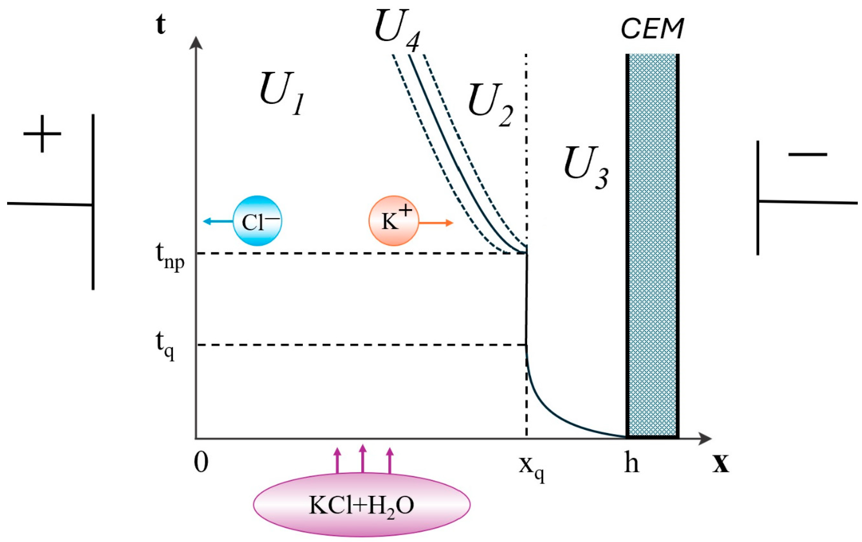
2.1. Diffusion Layer at the Cation-Exchange Membrane (CEM)

Let us consider the non-stationary transport of salt ions in the diffusion layer of an ion-exchange membrane (for short, CEM). Let $x=0$, corresponding to the depth of the solution (the outer boundary of the diffusion layer), and let $x=h$—the conventional interphase boundary of the electrolyte solution/CEM. For definiteness, we will consider an aqueous solution of 1:1 electrolyte, for example, NaCl or KCl. It is assumed that the concentration values are known in the depth of the solution, and the condition of local electroneutrality is satisfied. A constant value at the interphase boundary is set for cations, determined by the exchange capacity CEM, and for anions—the impermeability condition, i.e., CEM is considered ideally selective.

It is known that EMS are used and studied in two different modes:

(1)

In potentiodynamic (potentiostatic) mode, a potential drop $\mathsf{\Delta }\phi \left(t\right)$ is set, and the corresponding current density flowing through the electromembrane system (for example, a diffusion layer) is determined (in mathematical models, it is calculated from the found solution). Since it is the potential difference (drop) that matters, rather than specific values, an arbitrary constant can be set for the potential at one of the boundaries of the region under consideration, for example, zero at $x=h$, i.e., $\phi \left(t,h\right)=0$. Then, at $x=0$, we assume $\phi \left(t,0\right)=\mathsf{\Delta }\phi \left(t\right)$, where the function $\mathsf{\Delta }\phi \left(t\right)$ is specified. For example, when calculating the current–voltage characteristic (CVC), we assume $\mathsf{\Delta }\phi \left(t\right)={\phi }_n+d\cdot t$, where ${\phi }_n, d$ is the initial value (usually ${\phi }_n=0$) and the potential sweep rate, with the sweep rate being chosen small enough to ensure a quasi-stationary mode and coincidence with the CVC calculated for the potentiostatic mode with the required accuracy [29].

(2)

For the galvanodynamic (galvanostatic) mode, an external current $I\left(t\right)$ (current in the circuit including the EMS) is set, and the corresponding potential drop is determined. Below, we consider the galvanodynamic mode, which is determined by the galvanodynamic boundary condition, for example, at $x=0$, which was first proposed in [30].

The current mode is specified by the function $I\left(t\right)$. When calculating the CVC in the boundary condition (5), we assume $I\left(t\right)=I_n+d\cdot t$, where $I_n, d$ is the initial value (usually $I_n=0$) and the current density sweep rate, and, as in the potentiodynamic mode, the sweep rate is chosen to be small enough to ensure a quasi-stationary mode and coincidence with the CVC calculated for the galvanostatic mode with the required accuracy [30]. A simpler problem is when a constant external current is supplied, in this case $d=0$, and $I_0$ is the sub-limit or over-limit current. If, in the latter case, the initial state is a sub-limit, for example, as in [16,17], then we have an analogue of “shock electrodialysis”, when the charge wave or desalinated solution quickly propagates behind the wave front. In pulse modes [18,19,20,21,22,23,24,25,26,27], the current has a rectangular or triangular shape on a certain time interval and a zero value the rest of the time. The current mode determines the initial conditions in the boundary value problem of the mathematical model. The method proposed below can be used to obtain an analytical solution in all these cases.

Since it is the difference (drop) in potentials that matters, and not the specific values, an arbitrary constant can be set for the potential at one of the boundaries of the region under consideration, for example, zero at $x=h$.

2.2. Mathematical Model

The non-stationary transfer of salt ions in the diffusion layer of an ion-exchange membrane is described by a system of material balance and Nernst–Planck–Poisson equations [14,29,30]:

$${\displaystyle \frac{d{C}_i}{dt}}=-{\displaystyle \frac{d{j}_i}{dx}},i=1,2,$$

(1)

$$j_1=-{\displaystyle \frac{F}{RT}}{D}_1{C}_1{\displaystyle \frac{d\phi }{dx}}-D_1{\displaystyle \frac{d{C}_1}{dx}},$$

(2)

$$j_2={\displaystyle \frac{F}{RT}}{D}_2{C}_2{\displaystyle \frac{d\phi }{dx}}-D_2{\displaystyle \frac{d{C}_2}{dx}},$$

(3)

$${\displaystyle \frac{d^2\phi }{d{x}^2}}=-{\displaystyle \frac{F}{{\epsilon }_r}}(C_1-C_2),$$

(4)

where $j_1,j_2,C_1,C_2$ are the flux density and concentration of cations and anions in the solution, respectively, $D_1,D_2$ are the diffusion coefficients of cations and anions, $\phi$ is the electric field potential, ${\epsilon }_r$ is the dielectric constant of the solution, $F$ is the Faraday constant, $R$ is the gas constant, $T$ is the absolute temperature, and $t$ is the time.

2.3. Boundary Conditions

As noted above, at $x=0$, the salt ion concentrations $C_1(t,0)$, $C_2(t,0)$, are assumed to be known, and the local electroneutrality condition $C_1(t,0)-C_2(t,0)=0$ is satisfied in the depth of the solution, so we assume $C_1(t,0)=C_0$, $C_2(t,0)=C_0$.

We use the galvanodynamic boundary condition [30] for the potential, which is a generalization of Ohm’s law and relates the potential changes (electric field strength) to the external current value and the diffusion current determined by the ion concentration changes and the solution conductivity, which depends on the total salt ion concentration:

$${\displaystyle \frac{\partial \phi (t,0)}{\partial x}}=-{\displaystyle \frac{RT}{F^2}}\left({\displaystyle \frac{I(t)+F(D_1\frac{\partial C_1(t,0)}{\partial x}-D_2\frac{\partial C_2(t,0)}{\partial x})}{D_1{C}_1(t,0)+D_2{C}_2(t,0)}}\right).$$

(5)

At the interphase boundary at $x=h$, where $h$ is the thickness of the diffusion layer, we will assume the cation concentration to be known:

$$C_1(t,h)=C_{1K},$$

which is determined by the exchange capacity CEM. Let us assume that the membrane is ideally selective; then, the anion flux will be zero:

$${\left.\left({\displaystyle \frac{F}{RT}}{D}_2{C}_2{\displaystyle \frac{d\phi }{dx}}-D_2{\displaystyle \frac{d{C}_2}{dx}}\right)\right|}_{x=h}=0.$$

For the potential, the condition $\varphi (t,h)=0$ is specified (see above). The boundary conditions at are uniquely determined by the properties of the electrolyte solution, and at $x=h$ by the properties of the ion-exchange membrane. The boundary conditions given above are uniquely determined by the properties of the solution and the ion-exchange membrane and are widely used in modeling transfer processes [13,14], with the exception of the galvanodynamic boundary condition (5), developed by us.

2.4. Initial Conditions ($t=0$)

Initial conditions in the general case having the form:

$$C_1\left(0,x\right)=C_{10}(x),C_2\left(0,x\right)=C_{20}(x),\varphi \left(0,x\right)={\varphi }_0(x),$$

are selected based on the objectives of a specific study. If, for example, the process of formation of a space charge and similar problems are studied, then for the initial distributions of concentrations, potential should be sublimiting, and in other cases, they can be overlimiting. It is especially necessary to highlight processes with pulsed modes of the electric field. Initial conditions affect the structure of the diffusion layer, namely, its division into the ENR and SCR and, accordingly, the solution. As an example, let us assume that at the initial moment of time there is no external current and no concentration polarization (the concentrations are distributed uniformly); then, the initial conditions will take the form:

$$C_1\left(0,x\right)=C_2(0,x)=C_0,\varphi \left(0,x\right)=0.$$

(6)

In this case, the boundary value problem depends on the following variable dimensional input parameters: $h,C_0,C_{1k},d$.

3. Characteristic Quantities and Transition to Dimensionless Form

Let us move on to dimensionless quantities using the following formulas:

$$\begin{gathered} x^{(u)}={\displaystyle \frac{x}{h}},t^{(u)}={\displaystyle \frac{t}{t_0}},C_i^{(u)}={\displaystyle \frac{C_i}{C_0}},j_i^{(u)}={\displaystyle \frac{j_i}{j_0}},D_i^{(u)}={\displaystyle \frac{D_i}{D_0}}, \\ {\phi }^{(u)}={\displaystyle \frac{\phi }{{\phi }_0}},{\epsilon }^{(u)}={\displaystyle \frac{{\epsilon }_r}{{\epsilon }_0}},I^{(u)}={\displaystyle \frac{I}{I_0}},d^{(u)}={\displaystyle \frac{d}{d_0}} \end{gathered}$$

where (u) is the index of the dimensionless quantity, the subscript (0) indicates the characteristic quantities. If we take the following quantities as characteristic quantities, where $D_0={\displaystyle \frac{2D_1\cdot D_2}{D_1+D_2}}$ is the diffusion coefficient of the electrolyte, $I_0={\displaystyle \frac{F{D}_0{C}_0}{h}}={\displaystyle \frac{I_{np}}{2}}$, $I_{np}$ where is the limiting diffusion current, $j_0=F{I}_0$ is the ion flux corresponding to half the limiting current, $t_0={\displaystyle \frac{C_{0}h}{j_0}}={\displaystyle \frac{C_0{h}^2}{D_0{C}_0}}={\displaystyle \frac{h^2}{D_0}}$ is the ion diffusion time through the channel cross-section, ${\epsilon }_0={\displaystyle \frac{h^2\cdot F\cdot C_0}{{\varphi }_0}}$ is the typical value of the ionistor (an ionistor (supercapacitor, ultracapacitor, double-layer electrochemical capacitor) is an electrochemical device, a capacitor with an electrolyte, the “plates” of which are a double electric layer at the interface of the electrolyte solution/ion-exchange membrane; the typical capacity of an ionistor is several farads at a nominal voltage of 2–10 volts) capacitance (${\varphi }_0={\displaystyle \frac{RT}{F}}$ is the thermal potential), and $d_0={\displaystyle \frac{I_0}{t_0}}={\displaystyle \frac{F{D}_0{C}_0}{t_{0}h}}={\displaystyle \frac{F{D}_0^2{C}_0}{h^3}}$ is the characteristic value of the current density sweep rate, then, as is easy to verify, the dimensionless equations and boundary conditions will take the simplest form (Section 3).

4. Boundary Value Problem for a One-Dimensional Non-Stationary System of Equations of the NPP in Dimensionless Form

The boundary value problem for a one-dimensional non-stationary system of equations of the NPP, taking into account the above replacements, has a dimensionless form (the index “u” is omitted for simplicity):

$${\displaystyle \frac{d{C}_i}{dt}}=-{\displaystyle \frac{d{j}_i}{dx}},i=1,2,$$

(7)

$$j_i=-z_i{C}_i{D}_i{\displaystyle \frac{\partial \phi }{\partial x}}-D_i{\displaystyle \frac{\partial C_i}{\partial x}},z_1=-z_2=1,i=1,2$$

(8)

$$\epsilon {\displaystyle \frac{{\partial }^2\phi }{\partial x^2}}=-(C_1-C_2),$$

(9)

with boundary conditions

$$C_1(t,0,\epsilon )=C_2(t,0,\epsilon )=1,C_1(t,1,\epsilon )=C_{1m}$$

(10)

$${\displaystyle \frac{\partial \phi }{\partial x}}(t,0,\epsilon )=-\left({\displaystyle \frac{2I(t)+D_1\frac{\partial C_1}{\partial x}-D_2\frac{\partial C_2}{\partial x}}{D_1{C}_1+D_2{C}_2}}\right)(t,0,\epsilon ),\phi \left(t,1,\epsilon \right)=0.$$

(11)

The initial conditions in the general case are:

$$C_1\left(0,x,\epsilon \right)=C_{10}(x,\epsilon ),C_2\left(0,x,\epsilon \right)=C_{20}(x,\epsilon ),\varphi \left(0,x,\epsilon \right)={\varphi }_0(x,\epsilon ),$$

and are selected, as stated above, based on the objectives of the study.

For the particular case with which we begin the study, we obtain

$$C_1\left(0,x,\epsilon \right)=C_2(0,x,\epsilon )=1,\varphi \left(0,x,\epsilon \right)=0.$$

The boundary value problem (7)–(11) is a singularly perturbed boundary value problem [13,28,29,30] and at zero initial current contains two parameters $\epsilon$ and $d$. Since it contains a small parameter $\epsilon$ at the highest derivative in the Poisson Equation (9), it is related to “stiff” problems that are difficult to solve numerically [31]. The parameter $\epsilon$ can be represented as $\epsilon =2{(l_d/h)}^2$, where $l_{\mathrm{d}}=\sqrt{RT{\epsilon }_r/(2C_0{F}^2)}$ is the width of the quasi-equilibrium region of the space charge $U_3$ (the Debye length).

5. The Relationship Between the Currents in the Circuit and in the Diffusion Layer

The current density passed through the diffusion layer depends on time $I(t)$, while in the diffusion layer, the current density can change depending on the coordinate. Indeed, from the equations, it follows

$${\displaystyle \frac{\partial (C_1-C_2)}{\partial t}}=-{\displaystyle \frac{\partial (j_1-j_2)}{\partial x}}.$$

Let us replace the left side using the Poisson equation; then, we obtain

$$\epsilon {\displaystyle \frac{{\partial }^3\phi }{\partial t\partial x^2}}={\displaystyle \frac{\partial (j_1-j_2)}{\partial x}}.$$

Let us integrate this equation $x$ once; then,

$$\epsilon {\displaystyle \frac{{\partial }^2\phi }{\partial t\partial x}}=j_1-j_2+a_0(t) \mathrm{or}$$

(12)

$$\epsilon {\displaystyle \frac{{\partial }^2\phi }{\partial t\partial x}}=I(t,x)+a_0(t),$$

(13)

where $I(t,x)=j_1-j_2$ is the local current in the diffusion layer, determined by the ion flow.

Let us write relation (13) as

$$-a_0(t)=-\epsilon {\displaystyle \frac{{\partial }^2\phi }{\partial t\partial x}}+I(t,x).$$

Then, we transform the expression

$$-\epsilon {\displaystyle \frac{{\partial }^2\phi }{\partial t\partial x}}=\epsilon {\displaystyle \frac{\partial }{\partial t}}(-{\displaystyle \frac{\partial \phi }{\partial x}})=\epsilon {\displaystyle \frac{\partial E}{\partial t}}=I_c(t,x),$$

where $I_c(t,x)$ is the bias current associated with the formation and change of the SCR:

$$-a_0(t)=I_c(t,x)+I(t,x).$$

The expression on the right is the total current $I(t)$ and $a_0(t)=-I(t)$; therefore, (9) can be written as:

$$\epsilon {\displaystyle \frac{{\partial }^2\varphi }{\partial t\partial x}}=j_1-j_2-I(t).$$

(14)

6. Stationary Boundary Value Problem

It is necessary to study the stationary case so we can understand the non-stationary effects. In [12,31,32,33,34,35], it was shown that the diffusion layer consists of the ENR, the SCR, and a small intermediate layer between them [36]. It is known that in the ENR, the potential is described with high accuracy by the formula $\phi (x)=\ln \left|Ix-I_{np}\right|+{\phi }_0$, where $I_{np}\approx 2D_1$ is the dimensionless limiting current [37]. In [37], it was shown that in the space charge region, the potential satisfies the nonlinear singularly perturbed equation:

$$\epsilon {\phi }_{xx}=-{\displaystyle \frac{\epsilon }{2}}{\phi }_x^2+{\displaystyle \frac{1}{D_1}}(Ix-I_{np}).$$

(15)

By transformation, $\phi =2\ln \psi$ was reduced to a linear differential equation of the second order

$$\epsilon {\psi }_{xx}={\displaystyle \frac{I}{2D_1}}(x-{\displaystyle \frac{I_{np}}{I}})\psi ,$$

By replacing $\tau =(x-{\displaystyle \frac{I_{lim}}{I}})/\sqrt{{\displaystyle \frac{2D_1\epsilon }{I}}}$, $\psi (x,\epsilon )=u(\tau )$, it was reduced to the well-known and well-studied Airy equation, $u_{\tau \tau }=\tau u$, and thus, the potential distribution in the SCR was investigated with exhaustive completeness. For example, using the asymptotics of the Airy functions, it was shown that far from the boundary layer at $x=1$ and the singular point $x={\displaystyle \frac{I_{np}}{I}}$, i.e., in the interval $({\displaystyle \frac{I_{np}}{I}},1)$, the solution approximately has the form:

$$\phi (x,\epsilon )=a-{\displaystyle \frac{2}{3I}}\sqrt{{\displaystyle \frac{2}{\epsilon D_1}}}{(Ix-I_{np})}^{{\displaystyle \frac{3}{2}}},$$

where $a$ is the constant of integration.

The same solution can be obtained directly from Equation (15), if in it we neglect, according to the theory of singularly perturbed problems, the highest derivative with a small parameter $\epsilon {\phi }_{xx}$, but retain the nonlinear term with a small parameter ${\displaystyle \frac{\epsilon }{2}}{\phi }_x^2$, i.e., solve the equation ${\displaystyle \frac{\epsilon }{2}}{\phi }_x^2={\displaystyle \frac{1}{D_1}}(Ix-I_{np})$.

In this article, these results are generalized to the non-stationary case.

7. Algorithm for Solving a Non-Stationary Boundary Value Problem

(1)

Analysis of the numerical solution

The boundary value problem (7)–(11) was numerically solved by the finite element method in the Comsol Multiphysics 6.1 environment for the values of the initial concentration of the electrolyte solution $C_0=1\mathrm{mol}/{\mathrm{m}}^3,10\mathrm{mol}/{\mathrm{m}}^3$ and the thickness of the diffusion layer h = 0.1 mm. It was analyzed under different modes: galvanodynamic (galvanostatic) and potentiodynamic (potentiostatic). In Figure 1, Figure 2, Figure 3, Figure 4, Figure 5, Figure 6, Figure 7, Figure 8 and Figure 9, all quantities are given in dimensional form.

(a)

Galvanostatic mode

Let us analyze the distribution of concentrations and space charge in the galvanostatic mode, assuming that the current is constant, i.e., $I=1.5I_{np}$ for initial concentrations C₀ = 1 mol/m³ and C₀ = 10 mol/m³, obtained by numerically solving the boundary value problem (7)–(11).

As can be seen from Figure 1 and Figure 2, the nature of the propagation of concentrations and space charge for different initial concentrations C₀ = 1 mol/m³ and C₀ = 10 mol/m³ is qualitatively the same. At first, the concentrations decrease nonlinearly, and the mode is sub-limiting up to a certain point in time $\tau$ (usually called the transition time). The transition time for solution concentrations C₀ = 1 mol/m³ and C₀ = 10 mol/m³ is τ = 2.23 s and 2.22 s, respectively. From Figure 2 we obtain that up to the moment of time the space charge is completely concentrated in the quasi-equilibrium SCR, the thickness of which is so small that it is not displayed in Figure 2. At $t>\tau$, an extended SCR arises [9], in which the values of ion concentrations become small (Figure 1 at $t=3,4\dots 20 \mathrm{s}$), and the space charge has a clearly defined local maximum (Figure 2), i.e., a charge wave is formed, moving from the membrane deep into the diffusion layer. Note that the maximum local value of the space charge does not change over time, although it depends on the concentration of the electrolyte. Over time, the process stabilizes, namely, the distribution of concentrations in the ENR becomes linear, and the space charge wave stabilizes. Thus, the ENR, which is in front of the leading edge of the wave, decreases over time to a certain size and then stabilizes.

Figure 1. Distributions of cation (solid lines) and anion (dashed lines) concentrations at different times t = 0 s, 1 s, …, 20 s, calculated at a constant current density for C₀ = 1 mol/m³ (a) and C₀ = 10 mol/m³ (b).

Figure 1. Distributions of cation (solid lines) and anion (dashed lines) concentrations at different times t = 0 s, 1 s, …, 20 s, calculated at a constant current density for C₀ = 1 mol/m³ (a) and C₀ = 10 mol/m³ (b).

Figure 2. Distributions of the space charge density $\rho =F(C_1-C_2)$ at different times t = 0 s, 1 s, …, 20 s, calculated at a current density $I=1.5I_{np}$ of C₀ = 1 mol/m³ (a) and C₀ = 10 mol/m³ (b).

Figure 2. Distributions of the space charge density $\rho =F(C_1-C_2)$ at different times t = 0 s, 1 s, …, 20 s, calculated at a current density $I=1.5I_{np}$ of C₀ = 1 mol/m³ (a) and C₀ = 10 mol/m³ (b).

Figure 3. Distributions of potential (a,c) and electric field strength (b,d) at different times t = 0 s, 1 s, …, 20 s, calculated at current density for C₀ = 1 mol/m³ (a,b) and C₀ = 10 mol/m³ (c,d).

Figure 3. Distributions of potential (a,c) and electric field strength (b,d) at different times t = 0 s, 1 s, …, 20 s, calculated at current density for C₀ = 1 mol/m³ (a,b) and C₀ = 10 mol/m³ (c,d).

Figure 4. Distributions of the space charge density $\rho =F(C_1-C_2)$ at different times t = 0 s, 1 s, …, 20 s, calculated at a current density for C₀ = 10 mol/m³ (red lines), 1 mol/m³ (green lines), 0.1 mol/m³ (blue lines) (a), (b)—enlargement of a fragment of (a).

Figure 4. Distributions of the space charge density $\rho =F(C_1-C_2)$ at different times t = 0 s, 1 s, …, 20 s, calculated at a current density for C₀ = 10 mol/m³ (red lines), 1 mol/m³ (green lines), 0.1 mol/m³ (blue lines) (a), (b)—enlargement of a fragment of (a).

(b)

Galvanodynamic mode

Let us analyze the distribution of concentrations and space charge in the galvanodynamic mode, assuming that the current density changes $I=0.001I_{np}t$, i.e., the current sweep rate $d=0.001I_{np}$ is for the initial concentrations of C₀ = 1 mol/m³ and C₀ = 10 mol/m³. As can be seen from Figure 3 and Figure 4, the nature of the distribution of concentrations and space charge for different initial concentrations of C₀ = 1 mol/m³ and C₀ = 10 mol/m³ is also qualitatively similar. However, there is a significant difference from the galvanostatic mode. In the galvanodynamic mode at low sweep rates, regardless of the initial concentration, as well as in the galvanostatic mode until the moment of time $t_{np}\approx 1000c$, the sub-limit mode is observed. At $t>t_{np}$, an extended SCR and, accordingly, a local maximum appear, and the space charge wave begins to move into the solution. The thickness of the extended SCR constantly increases, as does the value of the local maximum, while the concentration distribution continues to remain close to linear in the ENR. The thickness of the ENR gradually decreases.

Figure 5. Distributions of cation $C_1$ (solid lines) and anion $C_2$ (dashed lines) concentrations at different times t = 0 s, 200 s, …, 2000 s, calculated at a current density $I=0.001I_{np}t$ of C₀ = 1 mol/m³ (a) and C₀ = 10 mol/m³ (b).

Figure 5. Distributions of cation $C_1$ (solid lines) and anion $C_2$ (dashed lines) concentrations at different times t = 0 s, 200 s, …, 2000 s, calculated at a current density $I=0.001I_{np}t$ of C₀ = 1 mol/m³ (a) and C₀ = 10 mol/m³ (b).

Figure 6. Distributions of the space charge density at different times t = 0 s, 200 s, …, 2000 s, calculated at a current density of C₀ = 1 mol/m³ (a) and C₀ = 10 mol/m³ (b).

Figure 6. Distributions of the space charge density at different times t = 0 s, 200 s, …, 2000 s, calculated at a current density of C₀ = 1 mol/m³ (a) and C₀ = 10 mol/m³ (b).

Figure 7. Distributions of potential $\phi$ (a,c) and electric field strength $E=-\partial \phi /\partial x$ (b,d) at different times t = 0 s, 200 s, …, 2000 s, calculated at current density $I=0.001I_{np}t$ for C₀ = 1 mol/m³ (a,b) and C₀ = 10 mol/m³ (c,d).

Figure 7. Distributions of potential $\phi$ (a,c) and electric field strength $E=-\partial \phi /\partial x$ (b,d) at different times t = 0 s, 200 s, …, 2000 s, calculated at current density $I=0.001I_{np}t$ for C₀ = 1 mol/m³ (a,b) and C₀ = 10 mol/m³ (c,d).

(c)

Potentiostatic mode

Let us consider the propagation of concentrations and space charge in the potentiostatic mode, with a constant potential drop of 0.5 V (Figure 8a,b and Figure 9a,b) and 1 V (Figure 8c,d and Figure 9c,d) for initial concentrations C₀ = 1 mol/m³ (Figure 8a,c and Figure 9a,c) and C₀ = 10 mol/m³ (Figure 8b,d and Figure 9b,d), obtained by numerically solving the boundary value problem (7)–(10). A similar behavior of the propagation of concentrations and space charge for different initial concentrations C₀ = 1 mol/m³ and C₀ = 10 mol/m³ can be observed in Figure 8 and Figure 9. At first, a nonlinear decrease in concentration is observed up to a certain pre-limit moment of time t_lim. It follows from Figure 8 that the value t_lim for a potential drop of 0.5 V is between 0.03 and 0.05 s, and that for a potential drop of 1 V is between 0.01 and 0.01 s. Until the time t_lim, the space charge is completely concentrated in the quasi-equilibrium SCR (Figure 9). At t > t_lim, an extended SCR [9] occurs, in which the concentration values become small (Figure 8 at t = 0, 1, … 20 s), and the space charge has a clearly defined local maximum (Figure 9), the values of which decrease with time, i.e., a charge wave is formed, moving from the membrane deep into the diffusion layer. Note that the maximum local value of the space charge decreases after some time and depends on the concentration of the electrolyte. With time, the process stabilizes, namely, the concentration distribution in the electroneutrality region becomes linear, and the space charge wave stabilizes. Thus, the electroneutrality region, which is in front of the leading edge of the wave, decreases over time to a certain size and then stabilizes.

Figure 8. Distributions of cation $C_1$ (solid lines) and anion $C_2$ (dashed lines) concentrations at different times t = 0.01 s, 0.02 s, 0.03 s, 0.05 s, 0.1 s, 0.15 s, 0.2 s, 0.3 s, 0.5 s, 1 s, 2 s, 5 s, 10 s, 15 s, 20 s, calculated at a potential drop of 0.5 V for C₀ = 1 mol/m³ (a) and C₀ = 10 mol/m³ (b), at a potential drop of 1 V for C₀ = 1 mol/m³ (c) and C₀ = 10 mol/m³ (d).

Figure 8. Distributions of cation $C_1$ (solid lines) and anion $C_2$ (dashed lines) concentrations at different times t = 0.01 s, 0.02 s, 0.03 s, 0.05 s, 0.1 s, 0.15 s, 0.2 s, 0.3 s, 0.5 s, 1 s, 2 s, 5 s, 10 s, 15 s, 20 s, calculated at a potential drop of 0.5 V for C₀ = 1 mol/m³ (a) and C₀ = 10 mol/m³ (b), at a potential drop of 1 V for C₀ = 1 mol/m³ (c) and C₀ = 10 mol/m³ (d).

Figure 9. Distributions of the space charge density at different times t = 0.01 s, 0.02 s, 0.03 s, 0.05 s, 0.1 s, 0.15 s, 0.2 s, 0.3 s, 0.5 s, 1 s, 2 s, 5 s, 10 s, 15 s, 20 s at a potential drop of 0.5 V for C₀ = 1 mol/m³ (a) and C₀ = 10 mol/m³ (b), at a potential drop of 1 V for C₀ = 1 mol/m³ (c) and C₀ = 10 mol/m³ (d).

Figure 9. Distributions of the space charge density at different times t = 0.01 s, 0.02 s, 0.03 s, 0.05 s, 0.1 s, 0.15 s, 0.2 s, 0.3 s, 0.5 s, 1 s, 2 s, 5 s, 10 s, 15 s, 20 s at a potential drop of 0.5 V for C₀ = 1 mol/m³ (a) and C₀ = 10 mol/m³ (b), at a potential drop of 1 V for C₀ = 1 mol/m³ (c) and C₀ = 10 mol/m³ (d).

(d)

Potentiodynamic mode

Let us consider the distribution of concentrations and space charge in the potentiodynamic mode at a potential sweep rate of 0.1 V/s and different initial concentrations C₀ = 1 mol/m³ and C₀ = 10 mol/m³ (Figure 10 and Figure 11). As can be seen in Figure 10 and Figure 11, the nature of the distribution of concentrations and space charge for different initial concentrations C₀ = 1 mol/m³ and C₀ = 10 mol/m³ is also qualitatively similar. However, there is a significant difference from the potentiostatic mode, in which the maximum local value of the space charge decreases with time and depends on the concentration of the electrolyte. At the same time, at low sweep rates, the change in concentrations is nonlinear, regardless of the initial concentration; however, as in the potentiostatic mode up to a certain point in time $t_{np}$, a sub-limit mode is observed. In Figure 10 and Figure 11 the values $t_{np}$ are between 3 and 5 s, when the extended SCR and, accordingly, local maxima appear (footnote: At very low scan rates, local maxima may not exist, but the wave itself is formed and moves into the solution) and the space charge wave begins to move into the solution. The thickness of the extended SCR constantly increases, but the value of the local maximum does not, while the concentration distribution continues to remain close to linear in the ENR. The thickness of the ENR gradually decreases.

Figure 10. Distributions of cation $C_1$ (solid lines) and anion $C_2$ (dashed lines) concentrations at different times t = 0.01 s, 0.02 s, 0.03 s, 0.05 s, 0.1 s, 0.15 s, 0.1 s, 0.2 s, 0.3 s, 0.5 s, 1 s, 2 s, 3 s, 5 s, 10 s calculated at a potential scan rate of 0.1 V/s for C₀ = 1 mol/m³ (a) and C₀ = 10 mol/m³ (b).

Figure 10. Distributions of cation $C_1$ (solid lines) and anion $C_2$ (dashed lines) concentrations at different times t = 0.01 s, 0.02 s, 0.03 s, 0.05 s, 0.1 s, 0.15 s, 0.1 s, 0.2 s, 0.3 s, 0.5 s, 1 s, 2 s, 3 s, 5 s, 10 s calculated at a potential scan rate of 0.1 V/s for C₀ = 1 mol/m³ (a) and C₀ = 10 mol/m³ (b).

Figure 11. Distribution of space charge density at different times t = 0.1 s, 0.2 s, 0.3 s, 0.5 s, 1 … 10 s at a potential rate of 0.1 V/s for C₀ = 1 mol/m³ (a) and C₀ = 10 mol/m³ (b).

Figure 11. Distribution of space charge density at different times t = 0.1 s, 0.2 s, 0.3 s, 0.5 s, 1 … 10 s at a potential rate of 0.1 V/s for C₀ = 1 mol/m³ (a) and C₀ = 10 mol/m³ (b).

(2)

The structure of the diffusion layer in the CEM

Analysis of the numerical solution (Figure 1, Figure 2, Figure 3, Figure 4, Figure 5, Figure 6, Figure 7, Figure 8, Figure 9, Figure 10 and Figure 11) shows the complex structure of the diffusion layer and the presence of several regions with different asymptotic behavior of the solution:

In Figure 12, the region $U_1(t,x)$ is the ENR, where the relation $C_1(x,\epsilon )-C_2(x,\epsilon )\approx 0$ is satisfied with high accuracy. The region $U_2(t,x)$ is the extended SCR, it occurs at $t>t_{np}$, when $I(t)>I_{np}$. In this region, $C_1(t,x,\epsilon )>>C_2(t,x,\epsilon )$, $\left|j_1(t,x,\epsilon )\right|>>\left|j_2(t,x,\epsilon )\right|$. The region $U_3(t,x)$ is the region of quasi-equilibrium space charge (boundary layer at the CEM). In this region, the equalities $C_2(t,x,\epsilon )=0$, $j_2(t,x,\epsilon )=0$ are satisfied with high accuracy. The width $U_3(t,x)$ of the region $t=0$ at is 0 and rapidly increases and over time of the order of 10⁻⁵ s to a value $h-x_q$, where $x_q=h+h\sqrt{\epsilon }\ln \epsilon$. Let us denote this curve $l_q$. In many problems, the curvilinear boundary of the region $l_q$ between the regions $U_1(t,x)$ and $U_3(t,x)$ for constructing an asymptotic solution can be approximated by the straight line $x=x_q$, which is shown in the figure as a dotted line.

The region $U_4(t,x)$ is an intermediate layer between the ENR and the extended SCR. The width of this region is small, $C_1(t,x,\epsilon )>C_2(t,x,\epsilon )$, but their values are comparable. This region is a certain neighborhood of the curve $l_c=\{(t,x):t\ge t_{np},x=I_{np}/I(t)\}$. It will be shown below Figure 13 that all points of this curve are singular points (turning points) for the singularly perturbed equation for the potential in the SCR.

Let us denote the curve $l=l_q{\displaystyle \cup l_c}$, defining the boundary between the ENR and the SCR, and assume that there is a function $x=x_c(t)$ such that $l=\{(t,x):t\ge 0,x=x_c(t)\}$.

Figure 13. Graph of local maxima in the intermediate region $U_4(t,x)$ at $t\ge t_{np}$.

Figure 13. Graph of local maxima in the intermediate region $U_4(t,x)$ at $t\ge t_{np}$.

(3)

Asymptotic solution algorithm

Due to such a complex structure of the diffusion layer, the method of splicing asymptotic expansions, similar to [37], is used for the asymptotic solution.

In each of the regions, the solution is sought in its own way and then they are spliced, i.e., the boundaries of the regions and arbitrary functions included in the solutions are determined. First, the entire region is divided into three regions: ENR $U_1$ and SCR $U_2\cup U_3$, as well as an intermediate region $U_4$ between them. In ENR, the solution method has been known for a long time and is similar to [38], but here, unlike [32], the solution region is curvilinear and is constructed in a special way (see Section 5). In SCR, equations are derived for the potential without additional assumptions, which are then transformed to a singularly perturbed linear equation of parabolic type, which is much easier to study. Finding a simplified solution region, an exact solution, and angular boundary layers are described in detail in [39].

Remark 1.

The proposed solution algorithm can be used not only in the galvanodynamic mode, but also in the potentiodynamic mode. The main difference is that in the galvanodynamic mode, the current is specified, so this function is considered known in all equations and the asymptotic solution, for example, in lines 518 and 519. Under potentiodynamic conditions, this current still needs to be calculated using the potential drop, which, along with additional mathematical problems, also produces cumbersome formulas that are significantly less convenient to use.

8. Solution in the Field of Electroneutrality

The transformations of the Nernst–Planck equations with the electroneutrality condition and their solution in a rectangular region by introducing the equilibrium concentration, as noted above, have long been known [38]. However, here, the region is curvilinear and, in addition, the boundary condition on the curvilinear boundary, which must be consistent with the solution in the extended SPR, is unknown. In this sense, the boundary value problem for the equilibrium concentration presented below is formulated and solved for the first time.

(1)

Boundary value problem for the equilibrium concentration.

The condition of local (pointwise) electroneutrality is satisfied for the degenerate system of equations obtained at from the original system of equations. Thus, in the ENR, we have a system of equations

$${\displaystyle \frac{\partial {\overline{C}}_i}{\partial t}}=-{\displaystyle \frac{\partial {\overline{j}}_i}{\partial x}},i=1,2$$

$${\overline{j}}_i=-z_i{\overline{C}}_i{D}_i{\displaystyle \frac{\partial \overline{\phi }}{\partial x}}-D_i{\displaystyle \frac{\partial {\overline{C}}_i}{\partial x}},i=1,2$$

(16)

$${\bar{C}}_1-{\bar{C}}_2=0$$

The last equation allows us to introduce the equilibrium concentration ${\overline{C}}_1={\overline{C}}_2=\overline{C}$, using which we obtain from these equations the well-known diffusion equation:

$${\displaystyle \frac{\partial \overline{C}}{\partial t}}=D{\displaystyle \frac{{\partial }^2\overline{C}}{\partial x^2}},$$

(17)

where $D={\displaystyle \frac{2D_1{D}_2}{D_1+D_2}}$ is the diffusion coefficient of the electrolyte.

Let us define the domain $U=\{(t,x):t\ge 0,x\le x_c(t)\}$. Obviously, $U\supset U_1(t,x)$. Let us denote by $C(t,x)$ the solution of the boundary value problem in the domain $U$:

$$\begin{gathered} {\displaystyle \frac{\partial C}{\partial t}}=D{\displaystyle \frac{{\partial }^{2}C}{\partial x^2}}, \\ C(t,0)=1,C(t,x){|}_{(t,x)\in l}=0,C\left(0,x\right)=1. \end{gathered}$$

Then, we take $C(t,x)$ as the restriction $\overline{C}(t,x)$ to the ENR $U_1(t,x)$, and the right boundary of the ENR must still be determined. Obviously, we then obtain $\overline{C}(t,x)>0$ of the ENR. The numerical solution of the boundary value problem (7–10) does not depend on $\epsilon$, and is not difficult. Due to the curvilinearity of the domain, it is necessary to use generalized curvilinear coordinates [40], to find an analytical solution, so that the transformation $\xi =\xi (t,x),\eta =\eta (t,x)$ maps the ENR into a rectangle $\mathsf{\Pi }=\{(\xi ,\eta ):0\le \xi ,\eta \le 1\}$.

Remark 2.

The current in the ENR does not depend on the spatial coordinate. Indeed, from ${\displaystyle \frac{\partial {\overline{C}}_i}{\partial t}}={\displaystyle \frac{D_1{D}_2}{D_1+D_2}}{\displaystyle \frac{{\partial }^2{\overline{C}}_i}{\partial x^2}}$, we have ${\displaystyle \frac{D_1{D}_2}{D_1+D_2}}{\displaystyle \frac{{\partial }^2{\overline{C}}_i}{\partial x^2}}=-{\displaystyle \frac{\partial {\overline{j}}_i}{\partial x}}$, $i=1,2$. Therefore, ${\displaystyle \frac{\partial ({\overline{C}}_1-{\overline{C}}_2)}{\partial t}}=-{\displaystyle \frac{\partial ({\overline{j}}_i-{\overline{j}}_2)}{\partial x}}$ or ${\displaystyle \frac{\partial (\overline{C}-\dot{C})}{\partial t}}=-{\displaystyle \frac{\partial ({\overline{j}}_i-{\overline{j}}_2)}{\partial x}}$. Whence ${\displaystyle \frac{\partial ({\overline{C}}_1-{\overline{C}}_2)}{\partial t}}=-{\displaystyle \frac{\partial ({\overline{j}}_i-{\overline{j}}_2)}{\partial x}}$, ${\displaystyle \frac{\partial (\overline{C}-\dot{C})}{\partial t}}=-{\displaystyle \frac{\partial ({\overline{j}}_i-{\overline{j}}_2)}{\partial x}}$, ${\displaystyle \frac{\partial ({\overline{j}}_i-{\overline{j}}_2)}{\partial x}}=0$, i.e., ${\overline{j}}_i-{\overline{j}}_2=\overline{I}(t)$. Since the Faraday current flows through the diffusion layer (see above) $I(t)$, then $I(t)=\overline{I}(t)$, which obviously agrees with the equality of the bias current to zero in the ENR.

(2)

Calculation of potential in ENR

From Equation (16), for i = 1, (16) is subtracted for i = 2; then,

$$(D_1+D_2){\displaystyle \frac{\partial }{\partial x}}(\overline{C}{\displaystyle \frac{\partial \overline{\phi }}{\partial x}})+(D_1-D_2){\displaystyle \frac{{\partial }^2\overline{C}}{\partial x^2}}=0,$$

$${\displaystyle \frac{\partial }{\partial x}}(\overline{C}{\displaystyle \frac{\partial \overline{\phi }}{\partial x}})+{\displaystyle \frac{D_1-D_2}{D_1+D_2}}{\displaystyle \frac{{\partial }^2\overline{C}}{\partial x^2}}=0,$$

$$\overline{C}{\displaystyle \frac{\partial \overline{\phi }}{\partial x}}+{\displaystyle \frac{D_1-D_2}{D_1+D_2}}{\displaystyle \frac{\partial \overline{C}}{\partial x}}=q(t).$$

For calculation $q(t)$, we put in this equation $x=0$; then, from the boundary condition for $\overline{C}$, we obtain

$${\displaystyle \frac{\partial \overline{\phi }}{\partial x}}(t,0)=-{\displaystyle \frac{D_1-D_2}{D_1+D_2}}{\displaystyle \frac{\partial \overline{C}(t,0)}{\partial x}}+q(t).$$

This boundary condition for $\epsilon =0$ has the form

$${\displaystyle \frac{\partial \overline{\phi }}{\partial x}}(t,0)=-{\displaystyle \frac{I(t)}{(D_1+D_2)}}-{\displaystyle \frac{(D_1-D_2)}{(D_1+D_2)}}{\displaystyle \frac{\partial \overline{C}(t,0)}{\partial x}}.$$

Comparing it with the boundary condition for $\epsilon =0$, we obtain

$$q(t)=-{\displaystyle \frac{I(t)}{(D_1+D_2)}},$$

$$\overline{C}{\displaystyle \frac{\partial \overline{\phi }}{\partial x}}+{\displaystyle \frac{D_1-D_2}{D_1+D_2}}{\displaystyle \frac{\partial \overline{C}}{\partial x}}=-{\displaystyle \frac{I(t)}{(D_1+D_2)}}.$$

Integrating it by $x$, we obtain

$$\overline{\phi }(t,x)-\overline{\phi }(t,0)=-{\displaystyle \frac{D_1-D_2}{D_1+D_2}}\ln \overline{C}(t,x)-{\displaystyle \frac{I(t)}{(D_1+D_2)}}{\displaystyle \underset{0}{\overset{x}{\int }}{\displaystyle \frac{dx}{\overline{C}(t,x)}}}.$$

9. Derivation of Equation for the Potential in the SCR of the CEM

Directly from the selective properties of the CEM and the definition of the SPR, it follows that the relations $C_1>>C_2$, $j_1>>j_2$ are fulfilled; therefore, the Poisson Equation (4) and $\epsilon {\displaystyle \frac{{\partial }^2\phi }{\partial t\partial x}}=j_1-j_2-I(t)$ can be simplified in the SCR of the CEM:

$$\epsilon {\displaystyle \frac{{\partial }^2\phi }{\partial x^2}}=-C_1,$$

(18)

$$\epsilon {\displaystyle \frac{{\partial }^2\phi }{\partial t\partial x}}=j_1-I(t).$$

(19)

Considering the flow

$$j_1=-C_1{D}_1{\displaystyle \frac{\partial \phi }{\partial x}}-D_1{\displaystyle \frac{\partial C_1}{\partial x}}.$$

We write Equation (19) in the form

$$\epsilon {\displaystyle \frac{{\partial }^2\phi }{\partial t\partial x}}=-C_1{D}_1{\displaystyle \frac{\partial \phi }{\partial x}}-D_1{\displaystyle \frac{\partial C_1}{\partial x}}-I(t).$$

We replace $C_1$ in the right-hand side using (18); then, we obtain an equation for the potential in the SCR:

$$\epsilon {\displaystyle \frac{{\partial }^2\phi }{\partial t\partial x}}=\epsilon D_1{\displaystyle \frac{{\partial }^2\phi }{\partial x^2}}{\displaystyle \frac{\partial \phi }{\partial x}}+\epsilon D_1{\displaystyle \frac{\partial }{\partial x}}{\displaystyle \frac{{\partial }^2\phi }{\partial x^2}}-I(t).$$

Since functions with lower indices are no longer encountered below, for clarity of writing, it is convenient to use a simpler notation for derivatives as indices, in which the previous equation is written in the form:

$$\epsilon {\phi }_{tx}=\epsilon D_1{\phi }_{xx}{\phi }_x+\epsilon D_1{\phi }_{xxx}-I(t)$$

Integrating this equation with respect to the previous equation, we obtain a singularly perturbed quasilinear parabolic equation for the potential

$$\epsilon {\phi }_t=\epsilon D_1{\phi }_{xx}+\epsilon {\displaystyle \frac{D_1}{2}}{\phi }_x^2-I(t)x+b(t,\epsilon ).$$

(20)

From the splicing condition in the presence of a stationary regime, $b(t,\epsilon )\to I_{np},\hspace{0.17em}t\to +\infty$.

Equation (20) can be easily reduced to the non-homogeneous Burgers equation [41,42], which is one of the standard non-linear equations of mathematical physics, and therefore the Hopf–Cole transformation is applicable to it. Thus, in this work, a connection between the dynamics of the space charge, and, accordingly, all other characteristics of the transfer of salt ions in membrane systems with a powerful mathematical apparatus was established for the first time. It allows us to implement an accurate analytical solution of a number of non-linear partial differential equations. As is known [39,40,41,42], the theory of solitons, nonlinear acoustics, nonlinear optics, nonlinear wave processes in plasma, radiophysics, and electronics saw rapid development in their time due to the establishment of a deep mathematical commonality between the phenomena observed in systems of the most diverse nature and the interpenetration of various methods in different areas. And non-linear standard equations played an extremely important role in this.

At the overlimit current density $I(t)$, we have $I(t)x-b(t,\epsilon )>0$ in the SCR and $I(t)x-b(t,\epsilon )<0$ in the ENR. Consequently, the boundary of the ENR and the SCR is the curve {$I(t)x-b(t,\epsilon )=0$}, and the intermediate layer is some small neighborhood of this curve. The form of the curve obviously depends on the current mode $I(t)$ and is analyzed below.

10. Analytical Solution of the Equation for $\mathit{\phi }$ Inside the Region ${\mathit{U}}_{\mathbf{2}}(\mathit{t},\mathit{x})$

Equation (20) can be solved in a simplified manner, similar to Remark 3 from [37].

(1)

Simplified analytical solution of the equation for $\varphi$ inside the region $U_2(t,x)$

In this equation, one cannot formally assume $\epsilon =0$ to find a solution to the degenerate equation. An approximate solution can be obtained by discarding the higher derivatives with a small factor, but keeping the nonlinear term of the equation with a small factor on the right-hand side. Then, we obtain the equation

$$\epsilon {\displaystyle \frac{D_1}{2}}{\phi }_x^2-I(t)x+b(t,\epsilon )=0.$$

Whence we obtain

$$\begin{gathered} \epsilon {\displaystyle \frac{D_1}{2}}{\phi }_x^2=I(t)x-b(t,\epsilon ), \\ {\phi }_x^2={\displaystyle \frac{2}{\epsilon D_1}}(I(t)x-b(t,\epsilon )), \\ {\phi }_x=\pm \sqrt{{\displaystyle \frac{2}{\epsilon D_1}}}{(I(t)x-b(t,\epsilon ))}^{{\displaystyle \frac{1}{2}}}, \\ \phi (t,x,\epsilon )=-{\displaystyle \frac{2}{3I(t)}}\sqrt{{\displaystyle \frac{2}{\epsilon D_1}}}{(I(t)x-b(t,\epsilon ))}^{{\displaystyle \frac{3}{2}}}+a(t,\epsilon ). \end{gathered}$$

The functions $b(t,\epsilon )$, $a(t,\epsilon )$ are determined from the condition of splicing of this solution in the extended SCR with solutions in neighboring regions of the quasi-equilibrium SCR and the intermediate layer.

Taking into account the formula $\epsilon {\displaystyle \frac{{\partial }^2\phi }{\partial x^2}}=-C_1$, we obtain

$$C_1(t,x,\epsilon )=\sqrt{{\displaystyle \frac{\epsilon }{2D_1}}}{\displaystyle \frac{I(t)}{\sqrt{I(t)x-b(t,\epsilon )}}}.$$

(21)

In dimensional form, the formulas for the potential and concentration are written as follows:

$$\begin{gathered} {\phi }_x=\pm \sqrt{{\displaystyle \frac{2RT}{{\epsilon }_r{D}_{1}F}}\left[I(t)x-b(t,\epsilon )F{D}_0{C}_0\right]}; \\ \phi (t,x,\mathit{\epsilon })=-\frac{2}{3I\left(t\right)}\sqrt{{\displaystyle \frac{2RT}{{\epsilon }_r{D}_{1}F}}}(I(t)x-b(t,\epsilon )F{D}_0{C}_0{)}^{\frac{3}{2}}+a(t,\epsilon )\frac{RT}{F}; \\ {C}_1(t,x)=\sqrt{{\displaystyle \frac{{\epsilon }_{r}RT}{2F^3{D}_1}}}{\displaystyle \frac{I(t)}{\sqrt{I(t)x-b(t,\epsilon )F{D}_0{C}_0}}}. \end{gathered}$$

As can be seen from Equation (21), the obtained solutions of Equation (20) can be valid only far from the points where $-I(t)x+b(t,\epsilon )=0$, i.e., to the right of the curve $l$. At the points of the curve, the solutions have a singularity, i.e., the points of the curve are turning points, and Equation (20) itself is a bisingular equation according to the classification [40].

(2)

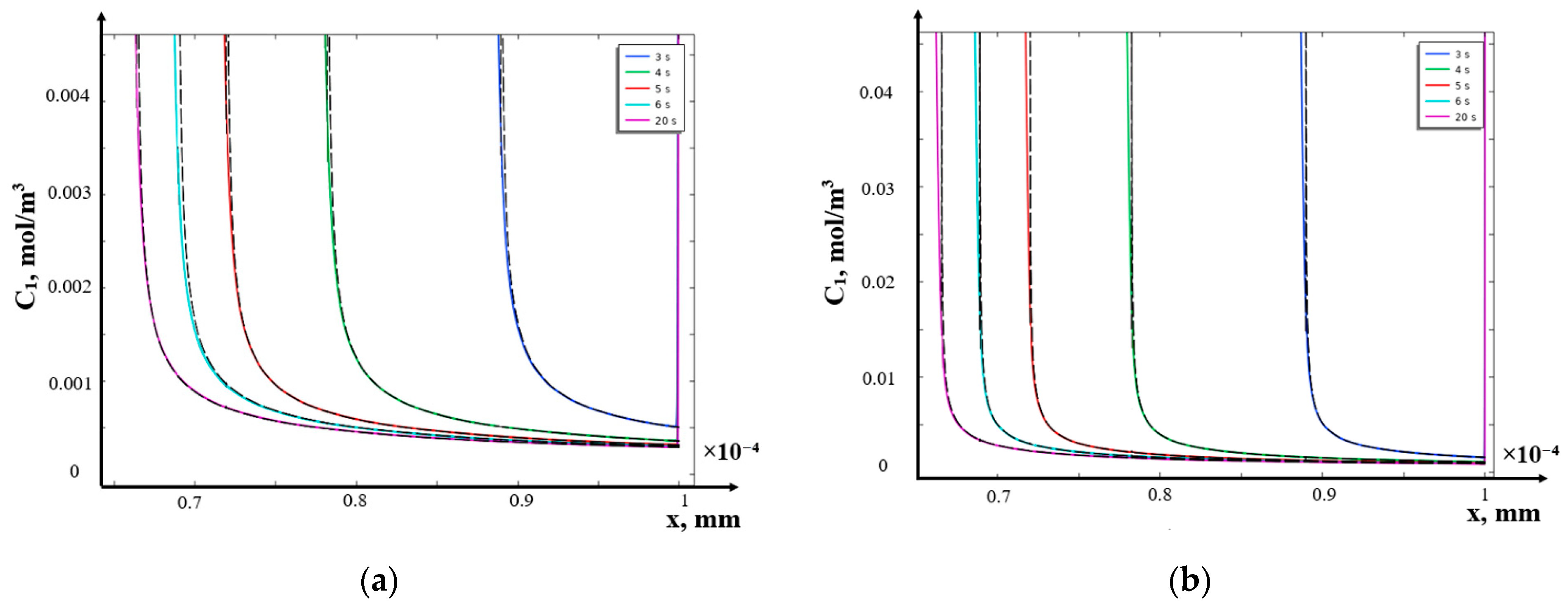
Comparison of the obtained analytical solution with the numerical solution inside the domain $U_2(t,x)$

To assess the accuracy of the obtained analytical solution, we will compare it with the numerical solution obtained by the finite element method in Comsol Multiphysics 6.1. As an example, we will use solutions for the galvanostatic mode at a constant current density $I=1,5I_{np}$ and a solution concentration of 1 mol/m³ and 10 mol/m³.

From Figure 14 it is evident that there is a fairly good qualitative and quantitative agreement between the numerical and analytical solutions. The approximation becomes worse as we approach the singular points, i.e., in the vicinity of the curve, which is, of course, natural, since $C_1(t,x,\epsilon )\to +\infty$ at $x\to {\displaystyle \frac{b(t,\epsilon )F{D}_0{C}_0}{I(t)}}+$ according to Equation (20), while the numerical solution remains limited. To refine the solution in the vicinity of the curve, it is necessary to use the asymptotics of the solution of a singularly perturbed linear inhomogeneous equation (see Section 11).

11. Reduction of Equation for $\mathit{\phi }$ in the SCR to an Auxiliary Linear Differential Equation of Parabolic Type

As noted above, Equation (20) can be applied to the inhomogeneous Burgers equation, and therefore, we apply Hopf–Cole transformation to it: setting $\phi =2\ln \psi$, we obtain the equation $\psi$.

$$2\epsilon {\displaystyle \frac{{\psi }_t}{\psi }}=-2\epsilon D_1{({\displaystyle \frac{{\psi }_x}{\psi }})}^2+2\epsilon D_1{\displaystyle \frac{{\psi }_{xx}}{\psi }}+2\epsilon D_1{({\displaystyle \frac{{\psi }_x}{\psi }})}^2-I(t)x+b(t,\epsilon ).$$

The terms containing $2\epsilon D_1{({\displaystyle \frac{{\psi }_x}{\psi }})}^2$ cancel each other out, and the equation becomes a linear equation of parabolic type:

$$\begin{gathered} 2\epsilon {\displaystyle \frac{{\psi }_t}{\psi }}=2\epsilon D_1{\displaystyle \frac{{\psi }_{xx}}{\psi }}-I(t)x+b(t,\epsilon ) \mathrm{or} \\ \epsilon {\psi }_t=\epsilon D_1{\psi }_{xx}+{\displaystyle \frac{1}{2}}(-I(t)x+b(t,\epsilon ))\psi . \end{gathered}$$

Thus, for the electric field potential in the SCR, we obtain [34], a bisingularly perturbed equation of parabolic type

$$\epsilon ({\psi }_t-D_1{\psi }_{xx})={\displaystyle \frac{1}{2}}(-I(t)x+b(t,\epsilon ))\psi .$$

For special cases of the function $I(t)$, for example, for direct current, this equation is reduced to a homogeneous equation, i.e., it admits an exact solution.

The Darboux transformation method has proven its effectiveness for solving the inhomogeneous heat conduction equation in general [37]. The application of the Darboux transformation in recent years has made it possible to obtain new solvable models of quantum mechanics. The connections of the Darboux transformation with the inverse scattering method and soliton theory are also interesting [38,39,40,41,42,43,44,45].

12. Diffusion Layer of an Anion Exchange Membrane (AEM)—Derivation of Equation for the Potential in the SCR at the AEM

Let us consider the diffusion layer at the AEM, where x = 0 corresponds to the conditional boundary of the AEM/solution, and x = 1 to the right boundary of the diffusion layer. In the SCR at the AEM, the relation is satisfied; therefore, Equation (4) and $\epsilon {\displaystyle \frac{{\partial }^2\phi }{\partial t\partial x}}=j_1-j_2-I(t)$ can be simplified:

$$\begin{gathered} \epsilon {\displaystyle \frac{{\partial }^2\varphi }{\partial x^2}}=C_2, \\ \epsilon {\displaystyle \frac{{\partial }^2\phi }{\partial t\partial x}}=-j_2-I(t). \end{gathered}$$

Let us rewrite the flow $j_2=C_2{D}_2{\displaystyle \frac{\partial \phi }{\partial x}}-D_2{\displaystyle \frac{\partial C_2}{\partial x}}$ using $\epsilon {\displaystyle \frac{{\partial }^2\phi }{\partial x^2}}=C_2$; then,

$$j_2=\epsilon D_2{\displaystyle \frac{\partial \phi }{\partial x}}{\displaystyle \frac{{\partial }^2\phi }{\partial x^2}}-\epsilon D_2{\displaystyle \frac{{\partial }^3\phi }{\partial x^3}}.$$

Substituting the flow into the equation

$$\begin{gathered} \epsilon {\displaystyle \frac{{\partial }^2\phi }{\partial t\partial x}}=-\epsilon D_2{\displaystyle \frac{\partial \phi }{\partial x}}{\displaystyle \frac{{\partial }^2\phi }{\partial x^2}}+\epsilon D_2{\displaystyle \frac{{\partial }^3\phi }{\partial x^3}}-I(t) \mathrm{we} \mathrm{obtain} \\ \epsilon {\displaystyle \frac{\partial \phi }{\partial t}}=-\epsilon {\displaystyle \frac{D_2}{2}}{({\displaystyle \frac{\partial \phi }{\partial x}})}^2+\epsilon D_2{\displaystyle \frac{{\partial }^2\phi }{\partial x^2}}-I(t)x+a(t,\epsilon ) \mathrm{or} \\ \epsilon {\phi }_t=-\epsilon {\displaystyle \frac{D_2}{2}}{({\phi }_x)}^2+\epsilon D_2{\phi }_{xx}-I(t)x+a(t,\epsilon ). \end{gathered}$$

Let us write this equation, similar to (20), as:

$$\epsilon ({\phi }_t-D_2{\phi }_{xx})=-\epsilon {\displaystyle \frac{D_2}{2}}{\phi }_x^2-I(t)x+a(t,\epsilon ).$$

This equation differs from Equation (20) by the sign of the nonlinear term. The change of variables $\phi =-2\ln \psi$ also leads this equation, as in item 8, to a linear equation of parabolic type.

13. Discussion

Boundary value problems for the Nernst–Planck–Poisson system of equations are of great importance in studying ion transport in EMS. At the same time, boundary value problems for stationary equations of the Nernst–Planck–Poisson systems have been studied much better than non-stationary ones, which is explained by significant mathematical difficulties. In the current article, new asymptotic solutions are given based on the general idea of obtaining a singularly perturbed nonlinear partial differential equation for the potential in the SCR and its transformation to a well-studied singularly perturbed linear parabolic equation. Approximate Equation (21) near the boundaries has a discrepancy with the numerical solution, which can be corrected using the exact solution of Equation (20). It is supposed to use new analytical solutions to study non-stationary processes of salt ion transport with exhaustive completeness and to identify effective desalination modes using ion-exchange membranes with structured surfaces in future works.

References

1. Jasielec, J.J. Electrodiffusion Phenomena in Neuroscience and the Nernst–Planck–Poisson Equations. Electrochem 2021, 2, 197–215. [Google Scholar] [CrossRef]
2. Liu, X.; Zhang, L.; Zhang, M. Studies on Ionic Flows via Poisson–Nernst–Planck Systems with Bikerman’s Local Hard-Sphere Potentials under Relaxed Neutral Boundary Conditions. Mathematics 2024, 12, 1182. [Google Scholar] [CrossRef]
3. Cartailler, J. Asymptotic of Poisson-Nernst-Planck Equations and Application to the Voltage Distribution in Cellular Micro-Domains. Analysis of PDEs [Math.AP]. Ph.D. Thesis, Université Pierre et Marie Curie—Paris VI, Paris, France, 2017. (In English). [Google Scholar]
4. Sun, L.; Liu, W. Non-localness of Excess Potentials and Boundary Value Problems of Poisson–Nernst–Planck Systems for Ionic Flow: A Case Study. J. Dyn. Differ. Equ. 2018, 30, 779–797. [Google Scholar] [CrossRef]
5. Chao, Z.; Xie, D. An improved Poisson-Nernst-Planck ion channel model and numerical studies on effects of boundary conditions, membrane charges, and bulk concentrations. J. Comput. Chem. 2021, 42, 1929. [Google Scholar] [CrossRef] [PubMed]
6. Liu, H.; Wang, Z. A free energy satisfying discontinuous Galerkin method for one-dimensional Poisson–Nernst–Planck systems. J. Comput. Phys. 2017, 328, 413–437. [Google Scholar] [CrossRef]
7. Gwecho, A.; Shu, W.; Mboya, O.; Khan, S. Solutions of Poisson-Nernst Planck Equations with Ion Interaction. Appl. Math. 2022, 13, 263–281. [Google Scholar] [CrossRef]
8. Grafov, B.M.; Chernenko, A.A. Theory of direct current flow through a binary electrolyte solution. Dokl. Akad. Nauk. SSSR 1962, 146, 135–138. [Google Scholar]
9. Urtenov, M.K.; Nikonenko, V.V. Analysis of the boundary-value problem solution of the Nernst-Planck-Poisson equations 1/1 electrolytes. Russ. Electrochem. 1993, 29, 314–324. [Google Scholar]
10. Uzdenova, A.; Kovalenko, A.; Urtenov, M.K.; Nikonenko, V. 1D mathematical modelling of non-stationary ion transfer in the diffusion layer adjacent to an ion-exchange membrane in galvanostatic mode. Membranes 2018, 8, 84. [Google Scholar] [CrossRef]
11. Kumar, P.; Rubinstein, S.M.; Rubinstein, I.; Zaltzman, B. Mechanisms of hydrodynamic instability in concentration polarization. Phys. Rev. Res. 2020, 2, 033365. [Google Scholar] [CrossRef]
12. Rubinstein, I.; Zaltzman, B. Electroconvection in electrodeposition: Electrokinetic regularization mechanisms of shortwave instabilities. Phys. Rev. Fluids 2024, 9, 053701. [Google Scholar] [CrossRef]
13. Lebedev, K.A.; Zabolotsky, V.I.; Vasil’eva, V.I.; Akberova, E.M. Mathematical modelling of vortex structures in the channel of an electrodialysis cell with ion-exchange membranes of different surface morphology. Condens. Matter Interphases 2022, 24, 483–495. [Google Scholar] [CrossRef] [PubMed]
14. Nikonenko, V.V.; Kovalenko, A.V.; Urtenov, M.K.; Pismenskaya, N.D.; Han, J.; Sistat, P.; Pourcelly, G. Desalination at overlimiting currents: State-of-the-art and perspectives. Desalination 2014, 342, 85–106. [Google Scholar] [CrossRef]
15. Kovalenko, A.V.; Nikonenko, V.V.; Chubyr, N.O.; Urtenov, M.K. Mathematical modeling of electrodialysis of a dilute solution with accounting for water dissociation-recombination reactions. Desalination 2023, 24, 483–495. [Google Scholar] [CrossRef]
16. Deng, D.; Aouad, W.; Braff, W.A.; Schlumpberger, S.; Suss, M.E.; Bazant, M.Z. Water purification by shock electrodialysis: Deionization, filtration, separation, and disinfection. Desalination 2015, 357, 77–83. [Google Scholar] [CrossRef]
17. Tian, H.; Alkhadra, M.A.; Bazant, M.Z. Theory of shock electrodialysis I: Water dissociation and electrosmotic vortices. J. Colloid Interface Sci. 2021, 589, 606–615. [Google Scholar] [CrossRef]
18. Rybalkina, O.; Solonchenko, K.; Chuprynina, D.; Pismenskaya, N.; Nikonenko, V. Effect of Pulsed Electric Field on the Electrodialysis Performance of Phosphate-Containing Solutions. Membranes 2022, 12, 1107. [Google Scholar] [CrossRef] [PubMed]
19. Gorobchenko, A.; Mareev, S.; Nikonenko, V. Mathematical Modeling of the Effect of Pulsed Electric Field on the Specific Permselectivity of Ion-Exchange Membranes. Membranes 2021, 11, 115. [Google Scholar] [CrossRef] [PubMed]
20. Nichka, V.; Mareev, S.; Pismenskaya, N.; Nikonenko, V.; Bazinet, L. Mathematical Modeling of the Effect of Pulsed Electric Field Mode and Solution Flow Rate on Protein Fouling during Bipolar Membrane Electroacidificaiton of Caseinate Solution. Membranes 2022, 12, 193. [Google Scholar] [CrossRef]
21. Lemay, N.; Mikhaylin, S.; Mareev, S.; Pismenskaya, N.; Nikonenko, V.; Bazinet, L. How demineralization duration by electrodialysis under high frequency pulsed electric field can be the same as in continuous current condition and that for better performances? J. Membr. Sci. 2020, 603, 117878. [Google Scholar] [CrossRef]
22. Mikhaylin, S.; Nikonenko, V.; Pourcelly, G.; Bazinet, L. Intensification of demineralization process and decrease in scaling by application of pulsed electric field with short pulse/pause conditions. J. Membr. Sci. 2014, 468, 389–399. [Google Scholar] [CrossRef]
23. Uzdenova, A.M.; Kovalenko, A.V.; Urtenov, M.K.; Nikonenko, V.V. Effect of electroconvection during pulsed electric field electrodialysis. Numerical experiments. Electrochem. Commun. 2015, 51, 1–5. [Google Scholar] [CrossRef]
24. Sistat, P.; Huguet, P.; Ruiz, B.; Pourcelly, G.; Mareev, S.A.; Nikonenko, V.V. Effect of pulsed electric field on electrodialysis of a NaCl solution in sub-limiting current regime. Electrochim. Acta 2015, 164, 267–280. [Google Scholar] [CrossRef]
25. Karlin, Y.V.; Kropotov, V.N. Electrodialysis separation of Na+ and Ca2+ in a pulsed current mode. Russ. J. Electrochem. 1995, 31, 472–476. [Google Scholar]
26. Mishchuk, N.A.; Koopal, L.K.; Gonzalez-Caballero, F. Intensification of electrodialysis by applying a non-stationary electric field. Colloids Surf. A Physicochem. Eng. Asp. 2001, 176, 195–212. [Google Scholar] [CrossRef]
27. Dufton, G.; Mikhaylin, S.; Gaaloul, S.; Bazinet, L. Positive impact of pulsed electric field on lactic acid removal, demineralization and membrane scaling during acid whey electrodialysis. Int. J. Mol. Sci. 2019, 20, 797. [Google Scholar] [CrossRef]
28. Newman, J. The polarized diffuse double layer. Trans. Faraday Soc. 1966, 61, 2229–2237. [Google Scholar] [CrossRef]
29. Uzdenova, A.M.; Kovalenko, A.V.; Urtenov, M.K.; Nikonenko, V.V. Theoretical Analysis of the Effect of Ion Concentration in Solution Bulk and at Membrane Surface on the Mass Transfer at Overlimiting Currents. Russ. J. Electrochem. 2017, 53, 1254–1265. [Google Scholar] [CrossRef]
30. Uzdenova, A.; Urtenov, M. Mathematical Modeling of the Phenomenon of Space-Charge Breakdown in the Galvanostatic Mode in the Section of the Electromembrane Desalination Channel. Membranes 2021, 11, 873. [Google Scholar] [CrossRef]
31. Uskov, V.I. Asymptotic solution of first-order equation with small parameter under the derivative with perturbed operator. Russ. Univ. Rep. Math. 2018, 23, 784–796, (In Russian, Abstract in English). [Google Scholar] [CrossRef]
32. Vasil’eva, A.B.; Butuzov, V.F. Singularly Perturbed Equations in Critical Cases; Moscow University: Moscow, Russia, 1978; p. 106. [Google Scholar]
33. Doolan, E.R.; Miller, J.J.H.; Schilders, W.H.A. Uniform Numerical Methods for Problems with Initial and Boundary Layers; Boole Press: Dublin, Ireland, 1980; 324p. [Google Scholar]
34. Listovnichy, A.V. Concentration polarization of the ionite membrane-electrolyte solution system in the overlimiting mode. Electrochemistry 1991, 27, 316–323. [Google Scholar]
35. Grafov, B.M.; Chernenko, A.A. The theory of the passage of a direct current through a solution of binary electrolyte. Dokl. Akad. Nauk. SSSR 1962, 153, 1110–1113. [Google Scholar]
36. Nikonenko, V.V.; Urtenov, M.K. On a generalization of the electroneutrality condition. Russ. J. Electrochem. 1996, 32, 195–198. [Google Scholar]
37. Kovalenko, S.A.; Urtenov, M.K. Asymptotic solution of the boundary value problem in the diffusion layer for the stationary system of Nernst—Planck—Poisson equations. Prospect. Sci. 2024, 6, 105–113. [Google Scholar]
38. Urtenov, M.; Chubyr, N.; Gudza, V. Reasons for the Formation and Properties of Soliton-Like Charge Waves in Membrane Systems When Using Overlimiting Current Modes. Membranes 2020, 10, 189. [Google Scholar] [CrossRef] [PubMed]
39. Fletcher, C.A.J. Computational Techniques for Fluid Dynamics; Springer: Berlin/Heidelberg, Germany, 1991; 401p. [Google Scholar]
40. Ilʹin, A.M. Matching of Asymptotic Expansions of Solutions of Boundary Value Problems; American Mathematical Society: Providence, RI, USA, 1992; 281p. [Google Scholar]
41. Matveev, V.B.; Salle, M.A. Darboux Transformations and Solitons; Springer: Berlin/Heidelberg, Germany, 1991. [Google Scholar]
42. Kudryavtsev, A.G.; Sapozhnikov, O.A. Determination of the exact solutions to the inhomogeneous Burgers equation with the use of the darboux transformation. Acoust. Phys. 2011, 57, 311–319. [Google Scholar] [CrossRef]
43. Kushner, A.G.; Matviichuk, R.I. Exact solutions of the Burgers–Huxley equation via dynamics. J. Geom. Phys. 2020, 151, 103615. [Google Scholar] [CrossRef]
44. Ryskin, N.M.; Trubetskov, D. Nonlinear Waves; Fizmatlit: Moscow, Russia, 2000; 296p. [Google Scholar]
45. Trubetskov, D.I.; McHedlova, E.S.; Anfinogentov, V.G.; Ponomarenko, V.I.; Ryskin, N.M. Nonlinear waves, chaos and patterns in microwave electronic devices. Chaos 1996, 6, 358–367. [Google Scholar] [CrossRef] [PubMed]
Figure 12. Schematic diagram of the diffusion layer (not to scale).
Mathematics 12 04040 g012
Figure 14. Distributions of cation concentrations in the extended SCR calculated numerically (solid lines) and using the asymptotic solution (20) (dashed lines) at a current density I = 1.5 I n p at time moments: 3 s, 4 s, 5 s, 6 s, 20 s for the initial concentration of the electrolyte solution C0 = 1 mol/m3 (a) and C0 = 10 mol/m3 (b).
Mathematics 12 04040 g014
Disclaimer/Publisher’s Note: The statements, opinions and data contained in all publications are solely those of the individual author(s) and contributor(s) and not of MDPI and/or the editor(s). MDPI and/or the editor(s) disclaim responsibility for any injury to people or property resulting from any ideas, methods, instructions or products referred to in the content.