Abstract
In this short communication, I share some personal thoughts on Sklar’s theorem and copulas after reading the original paper (Sklar, 1959) in French. After providing a literal translation of Sklar’s original statements, I argue that the modern version of ‘Sklar’s theorem’ given in most references has a slightly different emphasis, which may lead to subtly different interpretations. In particular, with no reference to the subcopula, modern ‘Sklar’s theorem’ does not provide the clues to fully appreciate when the copula representation of a distribution may form a valid basis for dependence modelling and when it may not.
MSC:
62H05
1. Introduction
In probability and statistics, copula methods have become ubiquitous when it comes to analysing, modelling and quantifying the dependence between variables; Genest et al. [1] provides a comprehensive up-to-date literature review on copula methods for approaching dependence in a variety of statistical settings. Systematically, any written (research paper) or verbal (conference talk) communication about copulas starts with a statement of the so-called ‘Sklar’s theorem’, establishing the existence of a copula for any multivariate probability distribution. After defining a d-dimensional copula () as a continuous cumulative distribution function supported on the unit hypercube with uniform marginals, the theorem is typically stated under a form equivalent to the following:
Theorem 0
(‘Sklar’s theorem’).
- 1.
- Let be a d-dimensional () distribution function with marginals . Then, there exists a d-dimensional copula C such thatfor all ; if each () is continuous, then C is unique; otherwise, C is uniquely determined on , where .
- 2.
- Conversely, if C is a d-dimensional copula and are univariate distribution functions, then the function defined via (1) is a d-dimensional distribution function with marginals .
(Here, denotes the extended real line ). This is the theorem as it is stated in Theorem 5.3 in McNeil et al. [2] and (for ) in Theorem 2.3.3 in Nelsen [3]. Statements in other main references on copulas, such as Theorem 1.1 in Joe [4], Theorem 2.2.1 in Durante and Sempi [5] or Theorem 2.3.1 in Hofert et al. [6], differ only slightly. The reference provided is invariably Sklar [7].
Now, not long ago, in the discussion following a seminar on copulas that I attended, the speaker argued that Sklar [7] was certainly the most cited unread statistical paper. The argument holds water if we put into perspective the facts that Sklar [7] is referenced each time copulas are introduced, leading to a huge number of citations (close to 11,000 at the time of writing, according to Google Scholar); and it is an ‘old’ paper in French, which was difficult to access for a long time, even after it was republished [8]. Thus, as Theorem 0 above is found (in English) in a multitude of other easily accessible sources, it may be reasonably conjectured that only a minor fraction of the authors citing Sklar [7] put in the effort to access and read the original text.
Admittedly, I was not part of that minor fraction until recently, and Theorem 0 was reported as is in Geenens et al. [9] and Geenens [10], with reference to [7] (which is very bad practice, for that matter). However, the previously mentioned discussion prompted me to read the original paper in French, only to find out that [7] does not contain any such ‘Sklar’s theorem’ under the above form—making the wider community aware of this fact may be the only purpose of this short note.
2. Sklar’s Statements
In fact, the paper [7] comprises five theorems, among which three (Théorème 1, Théorème 2 and Théorème 3), when combined, allow one to reconstruct and/or deduce Theorem 0. For convenience, we translate (bearing in mind that ‘traduire c’est trahir’—‘translating is betraying’—as my high-school English teacher used to say. Ironically, the statements in [7] were themselves, presumably, French translations of Sklar’s initial thoughts, making all this an interesting instance of the ‘broken telephone game’) here in English Sklar [7]’s Théorème 1, Théorème 2 and Théorème 3, as well as the definition of a copula appearing in the sequence (Définition 1). (The notations and footnotes are original from [7]. The three Théorèmes and the Définition appear in this order. Nothing is omitted between the statements, given without proofs).
Théorème 1 establishes the existence and uniqueness of the function that would later be called subcopula – Sklar [7] did not use that word, not introduced before (Definition 3, Schweizer and Sklar [12]). This subcopula, denoted H below to stay consistent with Théorème 1, is defined only on the ‘Cartesian product of the sets of values of ’, that is, in the notation of Theorem 0, and satisfies
Although no details are given, Théorème 2 states that the unique subcopula satisfying (2) may be extended ‘in general, in more than one way’ beyond into a function defined on the whole of the unit hypercube and satisfying Définition 1, such a function being called a copula. In other words, there exists at least one copula C coinciding exactly with the subcopula on :
Then, (1) follows immediately from (2) and (3). Evidently, the values taken by any such copula C outside are totally irrelevant, as they do not even appear in (1). All in all, Théorème 2 is akin to part of Theorem 0, while, clearly, Théorème 3 is its part 2.
Théorème 1. Let be an n-dimensional cumulative distribution function with margins . Let be the set of values of , for . Then there exists a unique function defined on the Cartesian product and such that |
Définition 1. We call (n-dimensional) copula any function , continuous, non-decreasing (in the sense of an n-dimensional cumulative distribution function), defined on the Cartesian product of n closed intervals and satisfying the conditions: |
| (Special cases of such functions were considered in [11]) |
Théorème 2. The function of Théorème 1 can be extended (in general, in more than one way) into a copula . An extension of , the copula satisfies the condition: |
Théorème 3. Let be given univariate cumulative distribution functions . Let be an arbitrary n-dimensional copula. Then the function defined as |
| is an n-dimensional cumulative distribution function with margins . |
What about part ? Sklar [7] does not make any specific mention of the uniqueness of the copula in the continuous case. Rather the contrary, Théorème 2 is stated with an explicit note about the non-uniqueness of the copula in general. Naturally, for a continuous univariate distribution , , thus if each () is continuous, then . In that case, (3) implies that the subcopula is a copula, and since there is no room for arbitrary extension, any copula C satisfying (1) must be that same subcopula, making such C unique. Hence, part follows from Théorèmes 1 and 2 and is not an add-on stricto sensu, but this was apparently not an essential point to make for Sklar [7].
This illustrates that Theorem 0 should not be regarded as just a concise re-statement of the sequence Théorèmes 1–3. The substance may be equivalent, but the form is not exactly the same, and this may lead to subtly different readings and interpretations. I outline my thoughts on this below.
3. Some Personal Comments
What is notable is that, although Sklar [7] gives a prominent place to the subcopula—with Théorème 1 explicitly devoted to it—it has totally disappeared from the ‘modern’ statement (Theorem 0), largely consigning it to oblivion. Indeed, in the above classical references, either the subcopula is introduced only in the technical lemmas leading to Theorem 0 (Lemma 2.3.4 in [3]; Lemma 2.3.3 in [5]), or it is not mentioned at all [2,4,6]. However, it is clear that the only informative part of the copula is the underlying subcopula; therefore, understanding completely the whys and wherefores of (1) seems conditional on the proper recognition of the role played by H. It is my opinion that short-circuiting the subcopula step, as in Theorem 0, induces overemphasis on the copula(s) C and, ultimately, unwarranted exploitation of (1) when . This is especially the case when it comes to analysing or modelling dependence, which is the main—if not only—application of Sklar’s theorem in statistics.
Remarkably, Theorem 0 does not make any reference to dependence; (1) is merely an analytical result providing an alternative representation of which may or may not be of any relevance. It is really the interpretation which we are willing to make of it which brings in the concept of dependence and relates it to copulas. Effectively, it appears from (1) that C is to capture how the marginals interlock inside , which it seems fair to call the ‘dependence structure’. This explains why, early on, copulas were called ‘dependence functions’, e.g., in (Definition 5.2.1, Galambos [13]) and Deheuvels [14,15].
However, for playing with the dependence structure of , the subcopula H is the only function worth examining: it always exists, it is always unique, and it always describes unequivocally, through (2), how to reconstruct from the marginals . Thus, with Théorème 1 in hand, it is not clear what the added value of the copula extension promised by Théorème 2 is—that same extension (1) implicitly but exclusively put forward by Theorem 0. This said, the fact that the subcopula H contains all necessary information for describing the dependence in does not imply that it is, in itself, a valid representation of that dependence. Indeed, defined on , the subcopula is, in general, not a stand-alone element which can be handled and analysed without reference to marginal distributions, and, therefore, cannot isolate a dependence structure as such. In fact, H must adjust to by definition—again, in general.
It so happens that, when all the marginal distributions are continuous, the subcopula takes a very specific form which is invariably a d-variate distribution function with continuous uniform margins on —this follows straightforwardly from the standard results on functions of random variables applied to (2), particularly the Probability Integral Transform (PIT) (if is a continuous variable with cumulative distribution , then always). In this case, the subcopula is a copula as per Définition 1, so (and (1) ≡ (2)) as observed above, but even more importantly this (sub)copula is ‘marginal-distribution-free’ (where ‘distribution-free’ is taken in the sense of [16]: free of the parent distribution. Thus, more specifically here, ‘marginal-distribution-free’, or ‘margin-free’, means free of the marginal distributions of the parent distribution ), also called ‘margin-free’. Unbound from any marginal interference, the (sub)copula can now be genuinely understood as capturing the heart of , that is, its dependence structure. The representation (1) is then particularly appealing, as it provides an explicit breakdown of a joint distribution into the individual behaviour of the variables of interest (captured by ) on one hand, and their interdependence structure (captured by C) on the other, with no overlap/redundancy between the two. The entire copula methodology for dependence modelling developed around this neat decomposition and its desirable consequences.
It cannot be stressed enough, though, that this pleasant situation only follows as a corollary of two favourable events which occur concurrently when and only when all the variables involved are continuous: first, the copula appearing in (1) is the subcopula, and second, that subcopula is margin-free. In all other non-continuous situations, any copula C satisfying (1) is nothing more than an arbitrary extension of the subcopula H in (2), which itself is not a satisfactory representation of the dependence of as it is not margin-free. The suitability of (1) for analysing and/or modelling dependence becomes, then, highly questionable. In effect, the validity of any attempt at dependence modelling based on the typical interpretation of (1) as a clear-cut decomposition ‘marginals vs. dependence’, is critically contingent on the continuity of all the variables—as a matter of fact, the early references which linked copulas to dependence through (1) [14,17,18], always considered continuous marginal distributions exclusively.
Yet, without any reference to the subcopula, the usual statement of ‘Sklar’s theorem’, as in Theorem 0, does not provide the clues to appreciate this. I questioned above the real benefit of the extension promised by Théorème 2 when we have Théorème 1. The question may be rephrased as: why did (1) become the universal baseline, in lieu of (2)? The only reason I see is that, since a copula is always a distribution supported on with standard uniform margins by definition, the function C in (1) appears as a standard familiar object (a cumulative distribution function) enjoying a nice invariance property (specifically: known marginals), as opposed to the function H in (2), whose exact nature is undefined and its specification requiring knowledge of . Yet, such invariance of C may only be granted in continuous cases (but then H enjoys the same desirable property, anyway), otherwise it is mostly a lure. In fact, the definition of C makes it into a blanket which conceals the fact that, ‘underneath’, its anchor points are fixed by H via (3). That the gaps between the nodes of may be filled in such a way that C maintains uniform margins is actually little more than an analytical artefact of no obvious relevance. Worse still, allowing those gaps to be filled may actually create more confusion than clarity and be misleading, as illustrated in Example 1 below.
What adds to the blur is part explicitly contrasting the continuous and non-continuous cases in terms of the (non-)uniqueness of the copula C in (1). This may give the feeling that this is the only notable difference between the two situations, and may consequently divert attention from other questions. Indeed, the lack of uniqueness of C and the ensuing problems of model unidentifiability have often been presented as the main hurdle for the practical use of copula methods outside the continuous framework, and have consequently been abundantly commented on [10,19,20,21,22]. In my current view, though, the only consequential difference between continuous and non-continuous cases is that the (sub)copula is margin-free in the former, and not in the latter—and this seems to have been much less frequently pinpointed as a problem on its own.
What has been discussed is all the ‘little annoyances’ which follow directly from this, e.g., the fact that copula-based dependence measures, such as Kendall’s or Spearman’s , depend on the margins in non-continuous settings ([23], Section 4 in [19]). Yet, these are only consequences of the lack of margin-freeness of C which, in itself, appears to me as the real predicament; in effect, we are losing the very reason-of-being of the copula approach, which is precisely its power to dissociate marginal behaviour and dependence structure via (1). For example, (Section 1.6, Joe [4]) motivates resorting to copulas over alternative multivariate models as follows: “(...) the copula approach has an advantage of having univariate margins of different types and the dependence structure can be modeled separately from univariate margins”. Yet, outside the continuous framework, this alleged separation between dependence structure and margins is clearly violated. All in all, it seems that copula methods applied to non-continuous distributions miss their own point entirely.
It is, therefore, my opinion that copula-like methods for analysing, modelling and quantifying dependence in non-continuous multivariate distributions should not be based on (1). I elaborated on this in [10], and proposed an alternative approach for discrete distributions. In a nutshell, the idea is to extract the information about dependence from the subcopula, and to reshape it under the form of a distribution with (discrete) uniform margins—hence ‘margin-free’—in order to define a discrete copula. A simple situation is explored below to illustrate the previous points.
Example 1.
Let be a bivariate Bernoulli vector; that is, for , , and the joint distribution p—i.e., , —are described by a table:
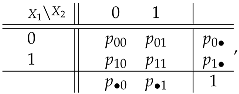 where , and (). As , there are initially three free parameters for p. Once the marginal values and are fixed, only one free parameter is left, the one describing the dependence inside p—cf., the -test for independence which articulates around one degree of freedom in this case. If the dependence parameter is to be ‘margin-free’, it must be (any one-to-one function of) the odds-ratio
([24], Theorem 6.3 in [25]). It is thus fair to identify the dependence structure to the value of ω in this case—see Section 4.3.1 of Geenens [26] for a thorough discussion.
where , and (). As , there are initially three free parameters for p. Once the marginal values and are fixed, only one free parameter is left, the one describing the dependence inside p—cf., the -test for independence which articulates around one degree of freedom in this case. If the dependence parameter is to be ‘margin-free’, it must be (any one-to-one function of) the odds-ratio
([24], Theorem 6.3 in [25]). It is thus fair to identify the dependence structure to the value of ω in this case—see Section 4.3.1 of Geenens [26] for a thorough discussion.
For this (obviously non-continuous) distribution, . Any copula C satisfying (1) may thus solely be identified on this grid. In fact, as any copula is fixed along the sides of (uniform margins; , , ), out of these 9 values only the ‘internal’ is informative (in agreement with the above, only one parameter may describe the dependence). Thus, Sklar’s representation (1) here reduces down to a single identity
For set values , this is, indeed, enough to identify by substitution the other values , and —hence, the whole distribution p. The odds ratio can then be written
For a given copula C, this is a continuous function of ; if we vary , generally changes accordingly. In fact, the only copula C guaranteeing to be constant in and is the Plackett copula, which was precisely designed for that purpose [27]. Thus, we may easily construct two bivariate Bernoulli distributions using the same copula C in (1)/(5), but showing very different dependence structures for different pairs of marginal parameters . Example 1.1 in Marshall [23] provides a compelling illustration of this. Clearly, it is not sensible to equate copulas and dependence structures here.
A subtle but consequential difference between (6) and (8), which justifies the different notations and , is that, unlike C, H is not defined elsewhere in the interior of than at . Thus, the idea of ‘varying the marginal parameters while keeping the same subcopula’ is groundless—if we were to amend the margins, we would have to consider another subcopula entirely, by definition. As opposed to (6), (8) makes it clear that the dependence structure (odds-ratio) induced by (5)/(7) is only meaningful when considering the given marginals. In fact, both H and C are margin-dependent to the exact same extent, but the ‘blanket’ nature of copulas, which cover the whole and always have uniform marginals, may give the dangerously comfortable feeling that it is not the case for C.
In order to represent the dependence structure of p in a margin-free way, and therefore mimic, at best, the definition of copulas in continuous settings, we may wish to exhibit the bivariate Bernoulli distribution with the same odds-ratio as p, but with Bern(1/2)-marginal distributions, i.e., uninformative uniform marginals in the class of Bernoulli distributions. It is a simple algebraic exercise to show that, for a given ,
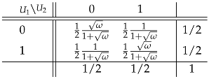 is such a distribution, and it is unique. This is what was called the ‘Bernoulli copula’ in Section 5 in Geenens [10]. Although evidently not a ‘copula’ according to Sklar [7]’s classical meaning—and not an element appearing in (1)/(5)—this Bernoulli copula enjoys all the pleasant properties which make copulas successful in continuous cases. For example, its associated correlation coefficient is a margin-free discrete analogue of Spearman’s ρ (Section 5.5 in [10])—which happens to be the correlation coefficient associated with the unique copula C of a continuous vector.
Funding
This research received no external funding.
Data Availability Statement
No new data were created or analyzed in this study. Data sharing is not applicable to this article.
Conflicts of Interest
The author declares no conflict of interest.
References
- Genest, C.; Okhrin, O.; Bodnar, T. Copula modeling from Abe Sklar to the present day. J. Multivar. Anal. 2023, in press. [Google Scholar] [CrossRef]
- McNeil, A.; Frey, R.; Embrechts, P. Quantitative Risk Management: Concepts, Techniques and Tools; Princeton University Press: Princeton, NY, USA, 2005. [Google Scholar]
- Nelsen, R. An Introduction to Copulas, 2nd ed.; Springer: New York, NY, USA, 2006. [Google Scholar]
- Joe, H. Dependence Modeling with Copulas; Chapman and Hall/CRC: Boca Raton, FL, USA, 2015. [Google Scholar]
- Durante, F.; Sempi, C. Principles of Copula Theory; CRC Press: Boca Raton, FL, USA, 2015. [Google Scholar]
- Hofert, M.; Kojadinovic, I.; Mächler, M.; Yan, J. Elements of Copula Modeling with R; Use R! Series; Springer Nature: Berlin/Heidelberg, Germany, 2018. [Google Scholar]
- Sklar, M. Fonctions de Répartition à n Dimensions et Leurs Marges; Publications de l’Institut de Statistique de l’Université de Paris: Paris, France, 1959; Volume 8, pp. 229–231. [Google Scholar]
- Bosq, D. L’article fondateur des copules. In Annales de l’Institut de Statistiques de l’Université de Paris; l’Institut de Statistiques de l’Université de Paris: Paris, France, 2010; Volume 54, pp. 3–6. [Google Scholar]
- Geenens, G.; Charpentier, A.; Paindaveine, D. Probit transformation for nonparametric kernel estimation of the copula density. Bernoulli 2017, 23, 1848–1873. [Google Scholar] [CrossRef]
- Geenens, G. Copula modeling for discrete random vectors. Depend. Model. 2020, 8, 417–440. [Google Scholar] [CrossRef]
- Féron, R. Sur les tableaux de corrélation dont les marges sont données. Cas de l’espace a trois dimensions. In Annales de l’Institut de Statistiques de l’Université de Paris; l’Institut de Statistiques de l’Université de Paris: Paris, France, 1956; Volume V, pp. 3–12. [Google Scholar]
- Schweizer, B.; Sklar, A. Operations on distribution functions not derivable from operations on random variables. Stud. Math. 1974, 52, 43–52. [Google Scholar] [CrossRef]
- Galambos, J. The Asymptotic Theory of Extreme Order Statistics; Wiley Series in Probability and Statistics—Applied Probability and Statistics Section; Wiley: Hoboken, NJ, USA, 1978. [Google Scholar]
- Deheuvels, P. La fonction de dépendance empirique et ses propriétés. Un test non paramétrique d’indépendance. Bull. L’AcadÉMie R. Belg. 1979, 65, 274–292. [Google Scholar] [CrossRef]
- Deheuvels, P. Non parametric tests of independence. In Statistique Non Paramétrique Asymptotique; Springer: Berlin/Heidelberg, Germany, 1980; pp. 95–107. [Google Scholar]
- Kendall, M.G.; Sundrum, R. Distribution-free methods and order properties. Rev. L’Institut Int. Stat. 1953, 21, 124–134. [Google Scholar] [CrossRef]
- Kimeldorf, G.; Sampson, A. Uniform representations of bivariate distributions. Commun.-Stat.-Theory Methods 1975, 4, 617–627. [Google Scholar] [CrossRef]
- Schweizer, B.; Wolff, E.F. On nonparametric measures of dependence for random variables. Ann. Stat. 1981, 9, 879–885. [Google Scholar] [CrossRef]
- Genest, C.; Nešlehová, J. A primer on copulas for count data. ASTIN Bull. 2007, 37, 475–515. [Google Scholar] [CrossRef]
- Trivedi, P.; Zimmer, D. A note on identification of bivariate copulas for discrete count data. Econometrics 2017, 5, 10. [Google Scholar] [CrossRef]
- Faugeras, O. Inference for copula modeling of discrete data: A cautionary tale and some facts. Depend. Model. 2017, 5, 121–132. [Google Scholar] [CrossRef]
- Nasri, B.; Rémillard, B. Identifiability and inference for copula-based semiparametric models for random vectors with arbitrary marginal distributions. arXiv 2023, arXiv:2301.13408. [Google Scholar]
- Marshall, A. Copulas, marginals and joint distributions. In Distributions with Fixed Marginals and Related Topics; Rüschendorf, L., Schweizer, B., Taylor, M., Eds.; Institute of Mathematical Statistics: London, UK, 1996; pp. 213–222. [Google Scholar]
- Edwards, A.W. The measure of association in a 2 × 2 table. J. R. Stat. Soc. Ser. A (Gen.) 1963, 126, 109–114. [Google Scholar] [CrossRef]
- Rudas, T. Lectures on Categorical Data Analysis; Springer: Berlin/Heidelberg, Germany, 2018. [Google Scholar]
- Geenens, G. Towards a universal representation of statistical dependence. arXiv 2023, arXiv:2302.08151. [Google Scholar]
- Plackett, R.L. A class of bivariate distributions. J. Am. Stat. Assoc. 1965, 60, 516–522. [Google Scholar] [CrossRef]
Disclaimer/Publisher’s Note: The statements, opinions and data contained in all publications are solely those of the individual author(s) and contributor(s) and not of MDPI and/or the editor(s). MDPI and/or the editor(s) disclaim responsibility for any injury to people or property resulting from any ideas, methods, instructions or products referred to in the content. |
© 2024 by the author. Licensee MDPI, Basel, Switzerland. This article is an open access article distributed under the terms and conditions of the Creative Commons Attribution (CC BY) license (https://creativecommons.org/licenses/by/4.0/).