Abstract
This paper proposes several methodologies whose objective consists of securing copula density estimates. More specifically, this aim will be achieved by differentiating bivariate least-squares polynomials fitted to Deheuvels’ empirical copulas, by making use of Bernstein’s approximating polynomials of appropriately selected orders; by differentiating linearized distribution functions evaluated at optimally spaced grid points; and by implementing the kernel density estimation technique in conjunction with a repositioning of the pseudo-observations and a certain criterion for determining suitable bandwidths. Smoother representations of such density estimates can further be secured by approximating them by means of moment-based bivariate polynomials. The various copula density estimation techniques being advocated herein are successfully applied to an actual dataset as well as a random sample generated from a known distribution.
Keywords:
copula density estimation; data modeling; nonparametric methodologies; polynomial approximations; pseudo-observations; Sklar’s theorem MSC:
62H05; 62G07
1. Introduction and Preliminary Considerations
1.1. Introduction
Copulas are principally utilized for modeling dependency features in multivariate distributions. Thus far, they have found applications in numerous fields of scientific investigation, including finance, reliability theory, machine learning, signal processing, geodesy, hydrology, and biostatistics. Of note, they are increasingly used in several areas of forecasting such as portfolio optimization, water systems management, values at risk, irradiation effects, and stock price projections. Such applications are discussed in the following recent papers among others: Quintero et al. [1], Kim et al. [2], Sreekumar et al. [3], Wang et al. [4], Karmakar and Khadotra [5], Müller and Reuber [6], Sahamkhadam and Stephan [7], and Wang et al. [8]. As well, a chapter of the monograph authored by Patton [9] is devoted to their use in connection with the forecasting of multiple time series.
Copulas enable one to represent the joint distribution of two or more random variables in terms of the marginal distributions and a specific correlation structure so that the effect of the dependence between the variables can be separated from the contribution of each of the marginals. This paper addresses the two-dimensional case, which is not overly restrictive as will be explained in Section 4. Certain definitions and results that will be needed in the sequel are reviewed next.
A bivariate copula function is a distribution whose support is the unit square, and whose marginals are uniformly distributed. More formally, a function is a bivariate copula if it satisfies the following properties:
For every , and
For every such that and ,
This last inequality ensures that is non-decreasing in both variables.
The following result, which was introduced by Sklar (1959) [10], constitutes a seminal contribution to the theory of copulas and its application.
Result 1
(Sklar’s Theorem). Let be the joint cumulative distribution function of the random variables X and Y whose continuous marginal distribution functions are denoted by and . Then, there exists a unique bivariate copula , such that
where is a joint cumulative distribution function having uniform marginals. Conversely, for any continuous cumulative distribution functions and and any copula , the function , as specified in Equation (1), constitutes a joint distribution function whose marginal distribution functions are and .
This result provides a technique for constructing copulas. Indeed, the function
is a bivariate copula, where the quasi-inverses and are given by
and
Copulas are invariant with respect to strictly increasing transformations. More specifically, letting X and Y be two continuous random variables whose associated copula is , if and are two strictly increasing functions and is the copula obtained from and , then for all
We shall denote the probability density function (pdf) corresponding to the copula by
The following relationship between the joint density function of X and Y, denoted by , and the associated copula density function can be readily obtained by differentiating the right-hand side of Equation (1) with respect to x and y:
where and respectively denote the marginal density functions of X and Y. Accordingly, the copula density function can be expressed as follows:
Given a random sample generated from the distributions of the continuous random variables X and let
where and are the usually unknown marginal cumulative distribution functions (cdf’s) of X and Y. Throughout this paper, X and Y are assumed to be continuous random variables, and n will denote the sample size. For the estimation of copulas having discrete marginals, the reader is referred to Genest and Nešlehová [11]. Now, since the underlying distributions of the variables are herein assumed to be continuous, the ’s are, in theory, all distinct, and so are the ’s. Should a dataset happen to contain replicates due to rounding, for instance, the observations could be randomly perturbed in a minimal way, which would ensure that the ranks associated with each variable will be distinct.
The pseudo-observations , are then defined in terms of the empirical marginal cdf’s denoted by and , that is,
where the empirical cdf’s (ecdf’s) are given by
with denoting the indicator function which is equal to 1 if condition is verified and 0 otherwise. Equivalently, one has
where is the rank of among and , the rank of among . Actually, the pseudo-observations form the support of the empirical copula probability mass function (pmf) which can only take on the values 0 and and is defined as follows:
the corresponding empirical copula (cdf), as specified by Deheuvels (1979) [12], being given by
Incidentally, is a consistent estimator of the copula . Additional theoretical results related to copulas are presented in Cherubini et al. [13,14], Denuit et al. [15], Joe [16], Nelsen [17], and Sklar (1959) [10], among others.
It is explained in the next subsection that it can prove advantageous to reposition the pseudo-observations.
1.2. Repositioning the Pseudo-Observations
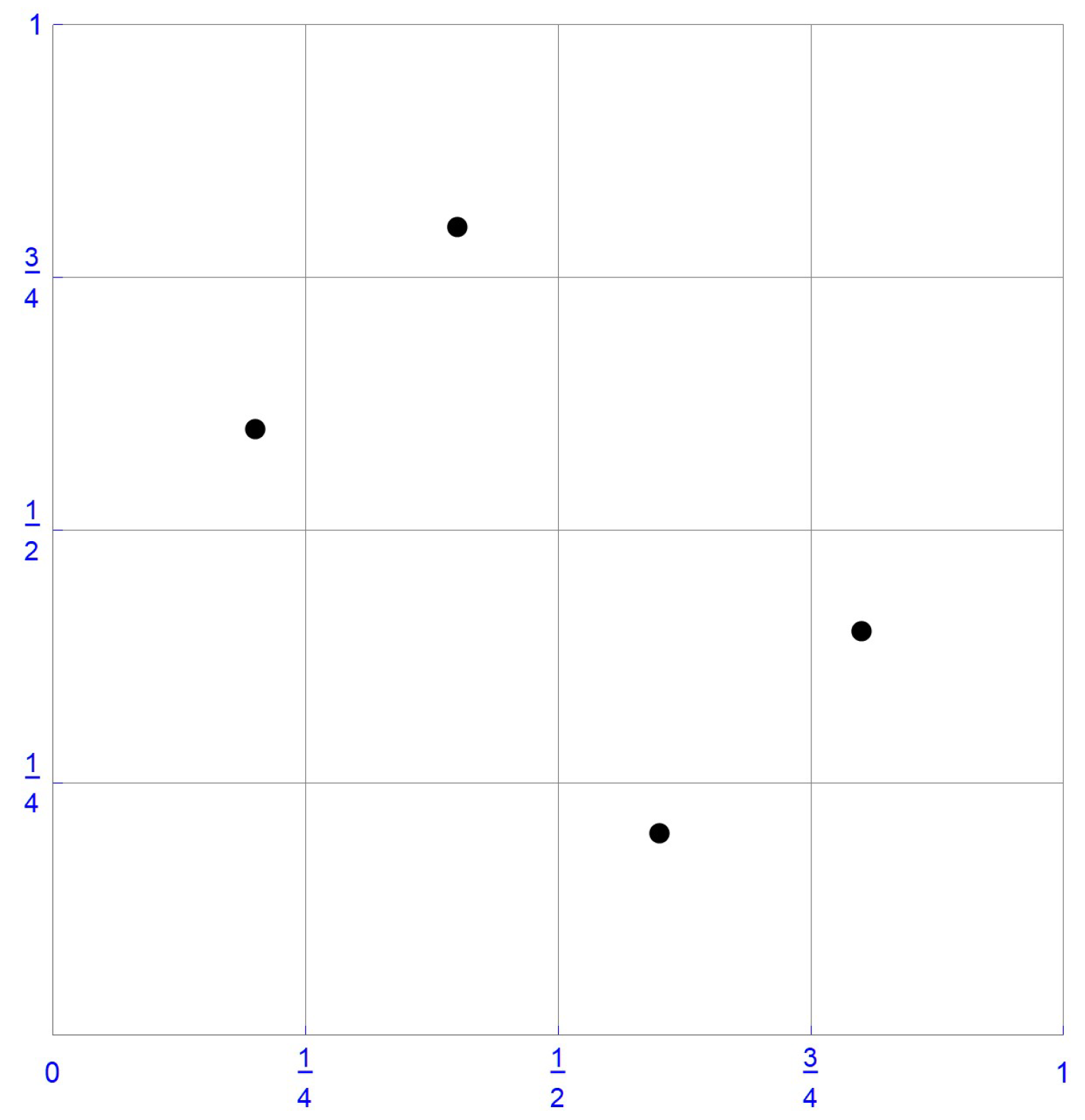
Given a random sample consisting of n bivariate observations, it is propounded that the favored positioning of the pseudo-observations ought to be at the center of the cell they occupy in an grid of the unit square. Thus, the corresponding centered pseudo-observations, that is, , are obtained by subtracting from each coordinate of .
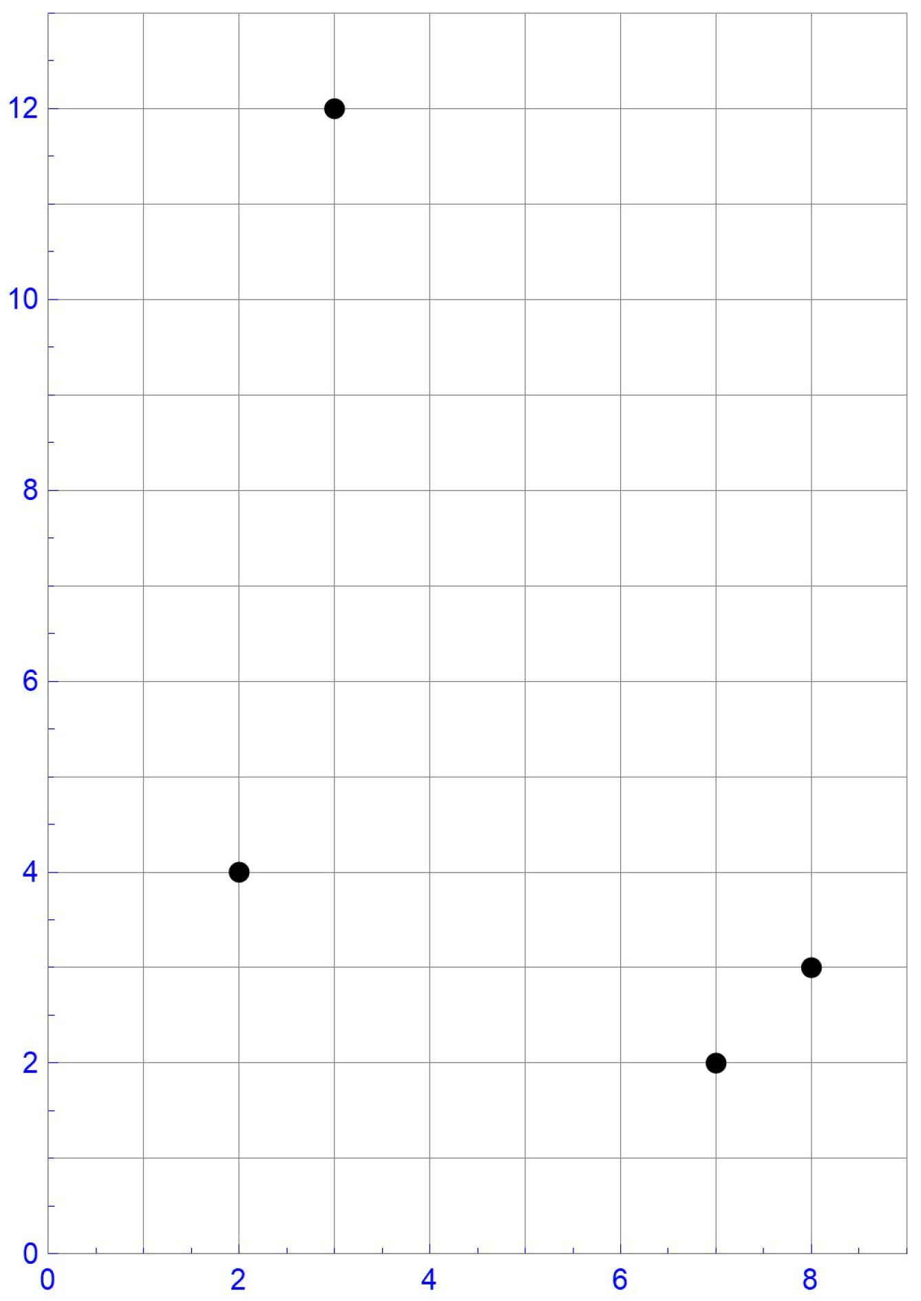
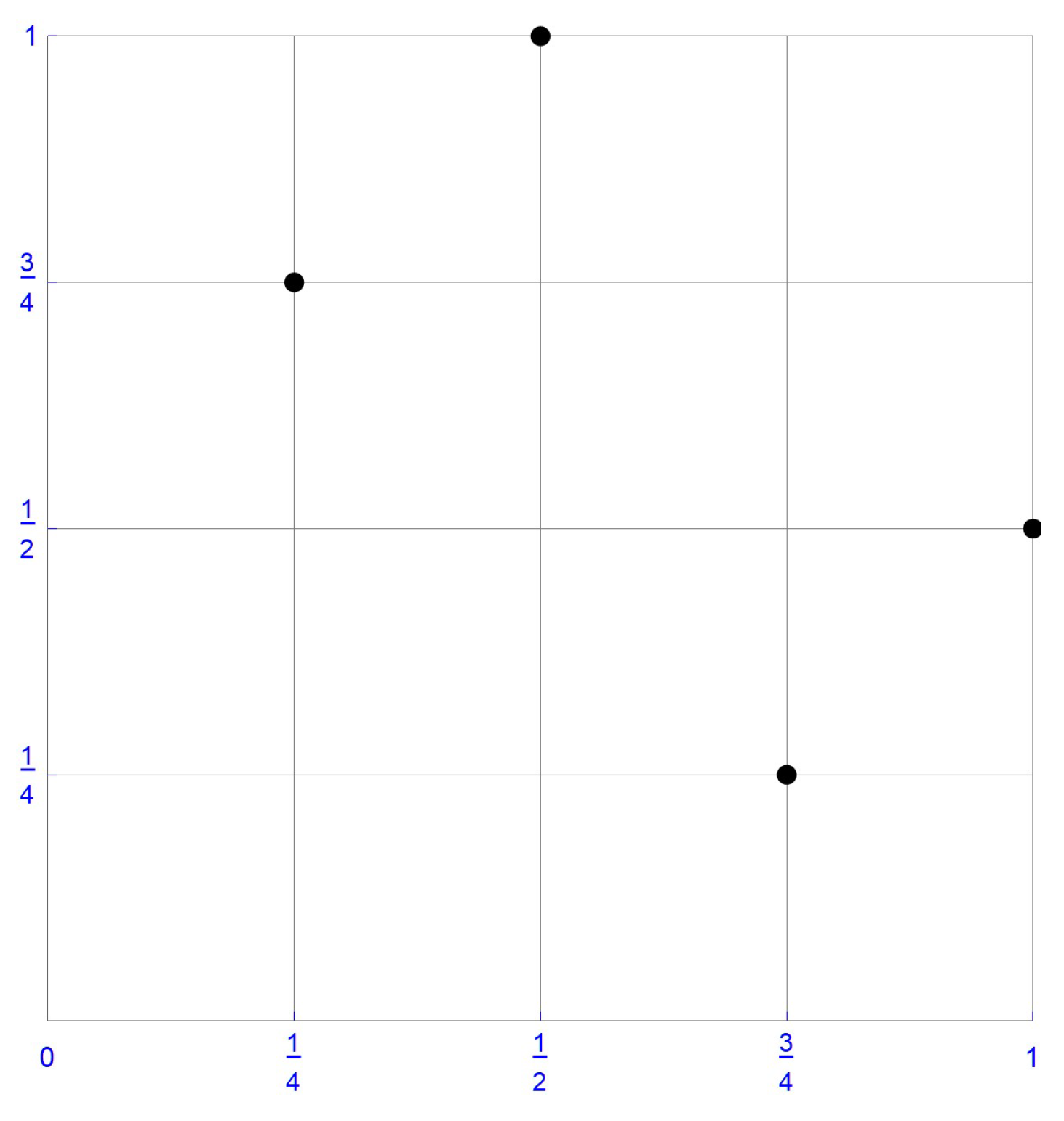
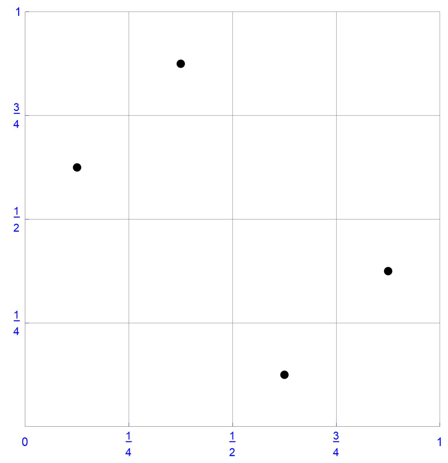
For illustrative purposes, consider the sample of size , which is plotted in Figure 1. In this instance, the ranks of the first component observations are , whereas those of the second component observations are . Accordingly, the pseudo-observations, , as defined in Equation (10), are . These pseudo-observations and the centered pseudo-observations obtained by subtracting 1/8 from each coordinate, that is, , are respectively shown in Figure 2 and Figure 3.
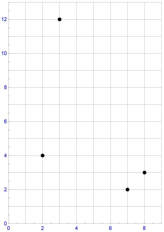
Figure 1.
The four data points.
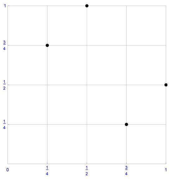
Figure 2.
The pseudo-observations.
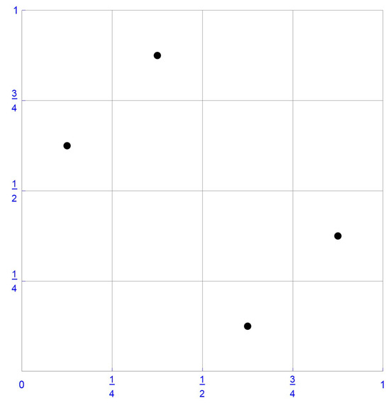
Figure 3.
Centered pseudo-observations.
When making use of pseudo-observations in the context of kernel density estimation, undesirable boundary effects ensues; as well, the resulting copula density estimates will be less concentrated near the origin and more concentrated near the coordinate (1,1) than they would be in the centered case. Recall that, ideally, copula marginals ought to be uniformly distributed.
An approach that is suggested in the literature for mitigating the edge effects consists of multiplying the pseudo-observations by , which, with , will produce the following points {, , }. These modified pseudo-observations are plotted in Figure 4. As can be seen from this graph, these points occupy haphazard positions within the corresponding grid cells, and their uneven distribution will result in a copula density that will be less concentrated in the vicinity of both ends of the unit intervals than it would be with centered pseudo-observations whose marginal probabilities are at the points , for each variable.
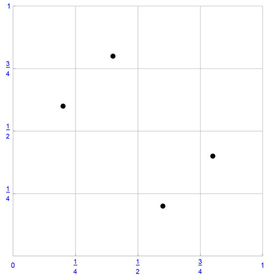
Figure 4.
Pseudo-observations ×.
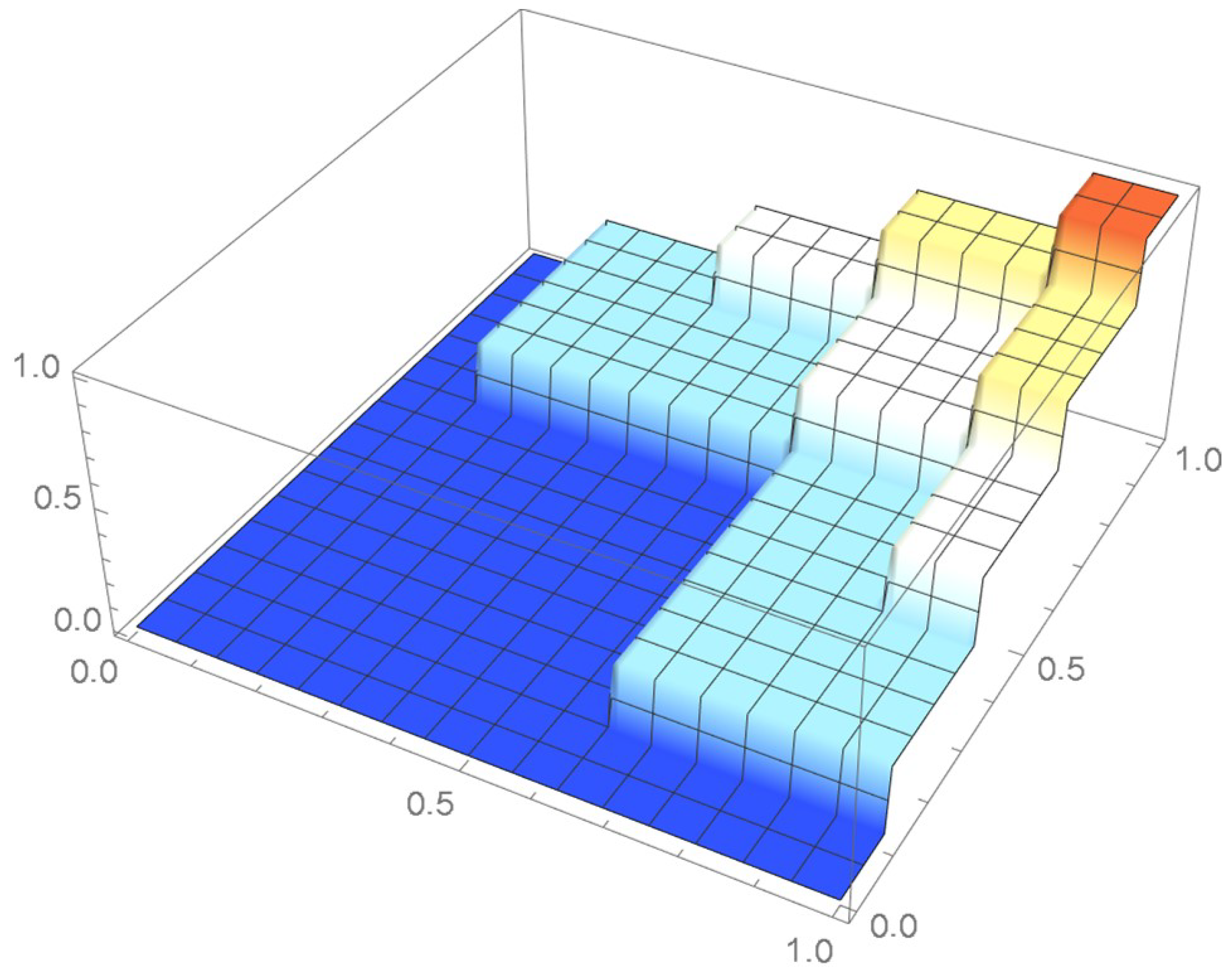
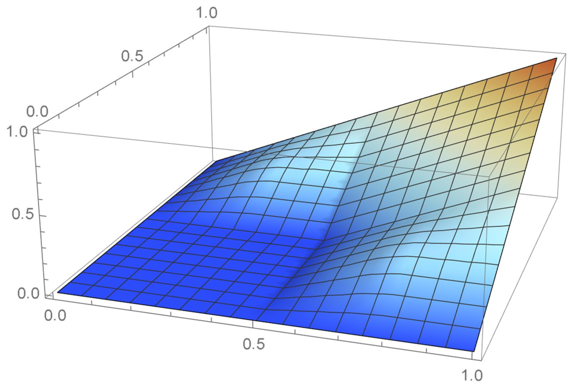
The empirical copulas as determined from the pmf of the pseudo-observations which is equal to 1/4 at the points shown in Figure 2 and, as obtained, the pmf of their centered counterparts shown in Figure 3, which is equal to 1/4 at those points, are respectively plotted in Figure 5 and Figure 6. The marginals are manifestly closer to being uniformly distributed in the latter case.
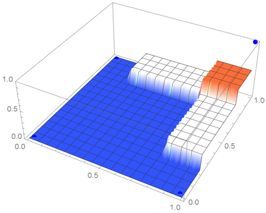
Figure 5.
Empirical copula as evaluated from the pseudo-observations.

Figure 6.
Empirical copula as evaluated from the centered pseudo-observations.
Wang and Fang [18] and Pérez et al. ([19], p. 100) discussed the following measure of divergence of a sample with respect to the distribution function , which is referred to as -discrepancy:
where denotes the empirical distribution function as determined from S and ℜ, the set of real numbers. We observe that is in fact the Kolmogorov–Smirnov statistic for assessing goodness-of-fit with respect to . It was established that in one dimension,
is the set of points having the lowest -discrepancy. In that sense, these n points form the most representative sample with respect to the distribution specified by . Thus, when is the distribution function of a uniform distribution on the unit interval, the sample of size n having the lowest -discrepancy is , which is precisely the support of each of the marginals of the distribution of the empirical copula pmf when the centered pseudo-observations are utilized.
Referring to the previous example, if one makes use of four cuboidal kernels whose height is 4 and whose bases are squares of dimension 1/4 × 1/4 that are centered at the centered pseudo-observations, , as defined at the beginning of this subsection, one obtains continuous uniform marginals on the unit interval from the resulting joint density function, which can be clearly observed by inspecting the copula density function appearing in Figure 7 and the corresponding bona fide copula plotted in Figure 8—obtained via integration of the joint density function shown in Figure 7. This clearly would not be the case with any other repositioning of the pseudo-observations. Uniform marginals could be similarly secured for bivariate samples of size n, in which case the cuboidal kernels would be of dimension . As there are n distinct ranks with respect to each coordinate, each row and each column of the grid of the unit square will contain exactly one pseudo-observation, whether centered or not.
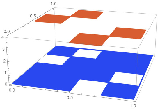
Figure 7.
Copula density estimate obtained from cuboidal kernels.

Figure 8.
Copula resulting from the cuboidal kernel density estimate.
Since the centered points are not lying on the boundary of the support of the copula, the edge issues being encountered in the context of kernel density estimation are ipso facto attenuated. Accordingly, we shall make use of the centered pseudo-observations whenever kernel density estimates (kde’s) are sought.
1.3. Moment-Based Polynomial Approximation Methodology
Once a copula density is determined by means of a nonparametric technique, it can be approximated or smoothed by a function consisting of the product of a bivariate base density function and a bivariate polynomial whose coefficients are determined from the joint moments of the copula distribution. The proposed procedure for achieving this is described in the next result which extends to two variables a proposition stated in Provost [20]. Essentially, once the joint moments of the target distribution, as defined in Equation (13)—be they exact or empirical—are secured, and those associated with an initial bivariate density approximation, , as specified in Equation (15), are determined, the density function of the target distribution, namely , can be approximated by taking the product of and a bivariate polynomial whose coefficients are obtained by solving the linear system (17). The methodology is described in the following result.
Result 2
(Moment-Based Bivariate Polynomial Approximations). Let be the density function of a bivariate continuous random variable defined in the rectangle . The joint moments of orders i and j obtained from are denoted as
Let be a base density function whose distributional features are analogous to those of . In the case of a copula, a uniformly distributed base density is generally suitable. The joint moments of orders i and j associated with are denoted as
Assuming that the sequence uniquely defines the distribution of , the density function of can be approximated by
where the polynomial coefficients can be specified by solving the following system of equations:
, which can be re-expressed as
Thus, given the joint moments associated with and one can determine the polynomial coefficients of by solving the system of linear equations specified by (17). The resulting polynomial function will be referred to as a moment-based bivariate polynomial approximation of degree n (in each variable).
It should be noted that this result can readily be extended to accommodate approximations of differing degrees in each variable. Such approximating polynomials can be utilized to express a copula estimate in a convenient form and, as the case may be, to smooth it. The base function can be a uniform density function or some other density function selected on the basis of the distributional features of the copula density. Whenever the copula density estimate to be approximated appears to exhibit an irregular pattern that cannot be related to a familiar copula density function, as is frequently the case, a uniform density function whose support area slightly exceeds that of the copula ought to be taken as the base density. Accordingly, unless specified otherwise, we will utilize such a base density for the purpose of approximating or smoothing copula density functions.
Degree n used in the polynomial adjustment should be selected so that provides an accurate approximation to the copula density estimate. In order to compare a copula density or distribution function estimate to a reference copula density or distribution function, we will make use of the integrated squared difference (ISD), which is equal to the integral of the square of their difference over the domain of interest. When the density estimates fluctuate erratically near the boundary, a subset of the unit square, namely , will be utilized for comparison purposes. Moreover, in order to ensure that the resulting density functions be bona fide within the unit square, the final approximations will be taken to be or when happens to take on negative values, as could possibly be the case with a polynomial approximation, with c denoting the normalizing constant.
To ensure that the polynomial approximations be positive only within a certain neighborhood of the set of pseudo-observations and zero elsewhere, we next introduce a technique for obtaining a suitable distributional support.
1.4. Determining the Support of a Copula Density Function
When a copula density function is directly estimated by a polynomial, as is the case for the differentiated least-squares copula estimates introduced in Section 2.1, or it is being approximated by means of a moment-based bivariate polynomial, as is the case in Section 2.4.2, some fluctuations may occur in certain areas located away from the pseudo-observations. To address this issue, a technique is being proposed for determining a distributional support denoted by , outside of which polynomial density estimates or approximants will be equal to zero.
The support is taken to be the union of all the points lying within a certain distance c of the centered pseudo-observations. Thus, denoting the centered pseudo-observations by the support of the copula density is defined as
where c, the radius of the circular neighborhood around each point, can be set as equal to 1/10 or another value that allows the density estimate to nearly reach zero on the boundary.
A bona fide copula density function is then obtained by multiplying its polynomial representation by the indicator function,
and normalizing the resulting function.
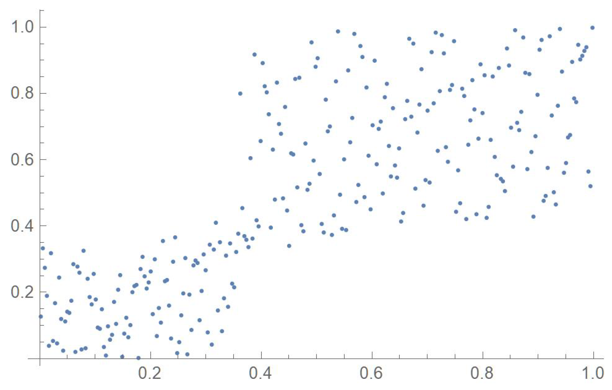
Consider the Old Faithful geyser eruption data which will be used throughout Section 2 for illustrative purposes. Scatter plots of the bivariate observations and the set of centered pseudo-observations are respectively shown in Figure 9 and Figure 10. The support of the distribution, that is, , as determined by letting , is plotted in orange in Figure 11. The polynomial copula density estimate appearing in Figure 12 was obtained by applying the differentiated least-squares technique introduced in Section 2.1. The bona fide copula density function, which is shown in Figure 13, was secured by bounding the original density estimate by the support and normalizing the resulting function.
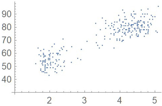
Figure 9.
Scatter plot of the data.
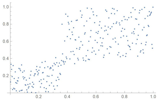
Figure 10.
Scatter plot of the centered pseudo-observations.
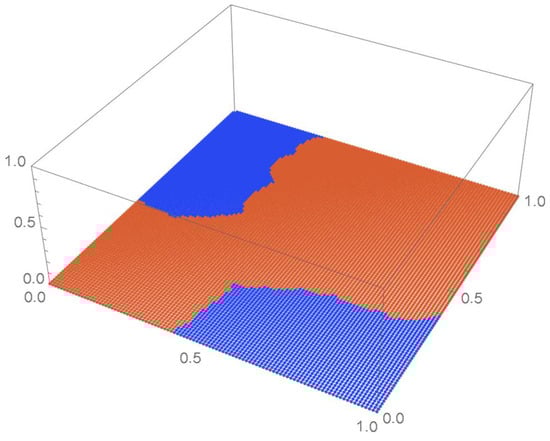
Figure 11.
, the support of the copula density.
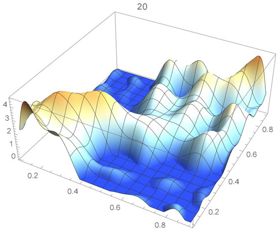
Figure 12.
Polynomial copula density estimate.

Figure 13.
Copula density estimate bounded by .
1.5. Structure of the Paper
The remainder of this paper is organized as follows. Section 2 proposes four nonparametric approaches for securing copula density estimates and specifies criteria for determining their associated tuning parameters. Additionally, Section 2.5 illustrates that a joint density estimate can be secured from a copula density estimate. The proposed copula density estimation techniques are then applied to a sample generated from a bivariate Student’s t distribution in Section 3. Several concluding remarks are then offered in the last section.
2. Methodologies for Estimating Copula Densities
2.1. Differentiated Least-Squares Copula Estimates
2.1.1. Introduction
Let denote the dataset at hand and be the associated empirical copula as specified in (12). A least-squares approximating polynomial of degree in each variable, which is denoted by , is fitted to the points , . The resulting polynomial is then differentiated with respect to u and v and normalized to obtain a copula density estimate denoted by , whose domain is delimited by the unit square. For a derivation of bivariate least-squares regression polynomials, the reader is referred to Fox ([21], Section 5.2.1).
On plotting the density estimates for one will notice that several successive plots turn out to be quite similar and that, past a certain value of t, higher-degree polynomials will exhibit noticeably larger fluctuations. That several graphs show nearly identical features over such a wide range of degrees provides a clear indication that the copula density functions so obtained are representative of the underlying distribution. Among these density estimates, the experimenter could select that which possesses the desired smoothness level or the polynomial of lower degree for the sake of parsimony. A suitable degree for could as well be determined more precisely by evaluating the integrated squared differences between copula estimates of orders t and and choosing the value of t beyond which the ISD’s no longer decrease markedly. Once normalized, the copula density estimate of the selected degree will be a bona fide density estimate, which could then be utilized as a yardstick to calibrate the tuning parameters of density functions resulting from the application of alternative methodologies.
2.1.2. An Illustrative Example
For comparison purposes, all the proposed copula density estimation techniques will be applied to the Old Faithful geyser eruption data, which consists of 272 bivariate observations whose first component represents the duration of an eruption in minutes and the second one, the waiting time to the next eruption in minutes. As can be seen from recently published articles such as Howlett [22] and Keller et al. [23], this dataset, as well as related ones, are still of current interest as they are required to understand the subsurface systems that give rise to the geysers. We selected this hydrogeological dataset, noting that its empirical copula is not as typical as those generally associated with datasets arising, for instance, in financial modeling, environmetrics, or epidemiology. The four nonparametric copula density estimation methodologies advocated in this and the next three subsections, which are also shown to be successful in modeling a challenging distribution in Section 3, would presumably apply to sets of observations originating from a variety of disciplines.
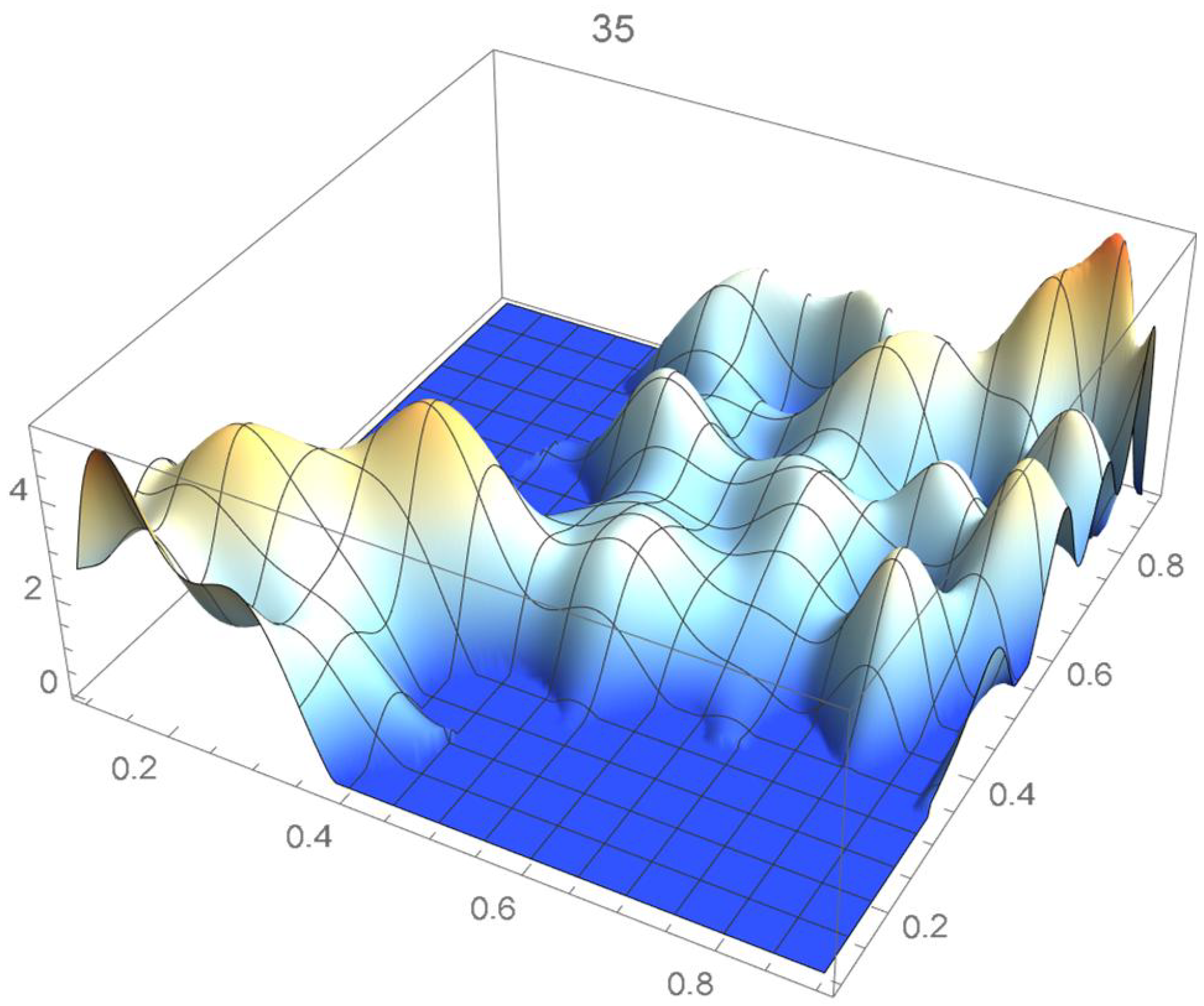
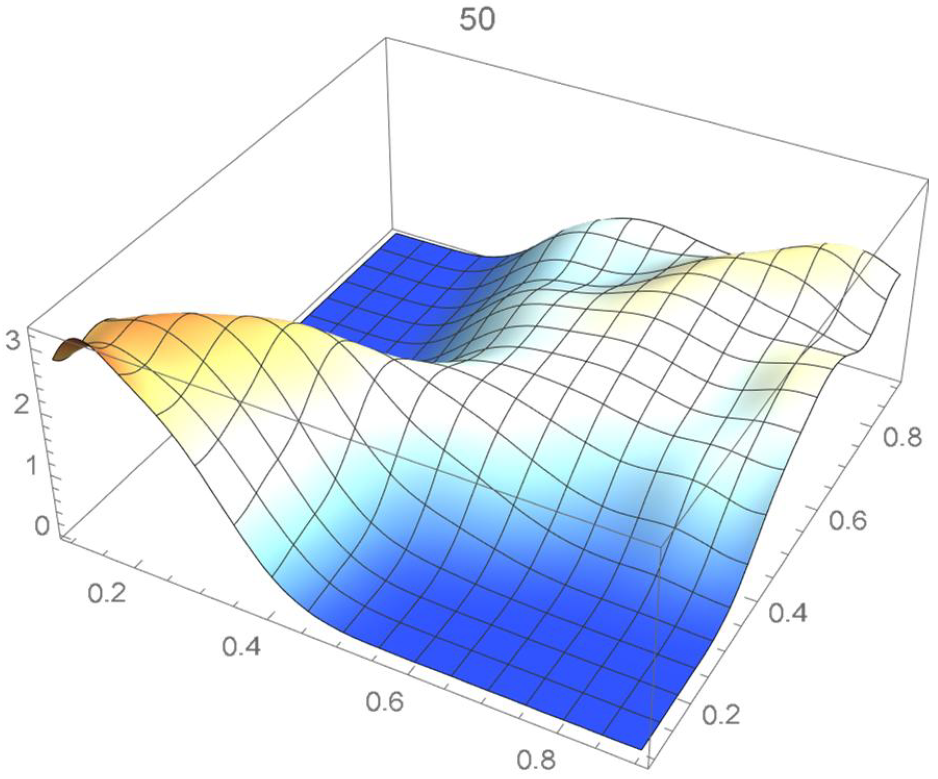
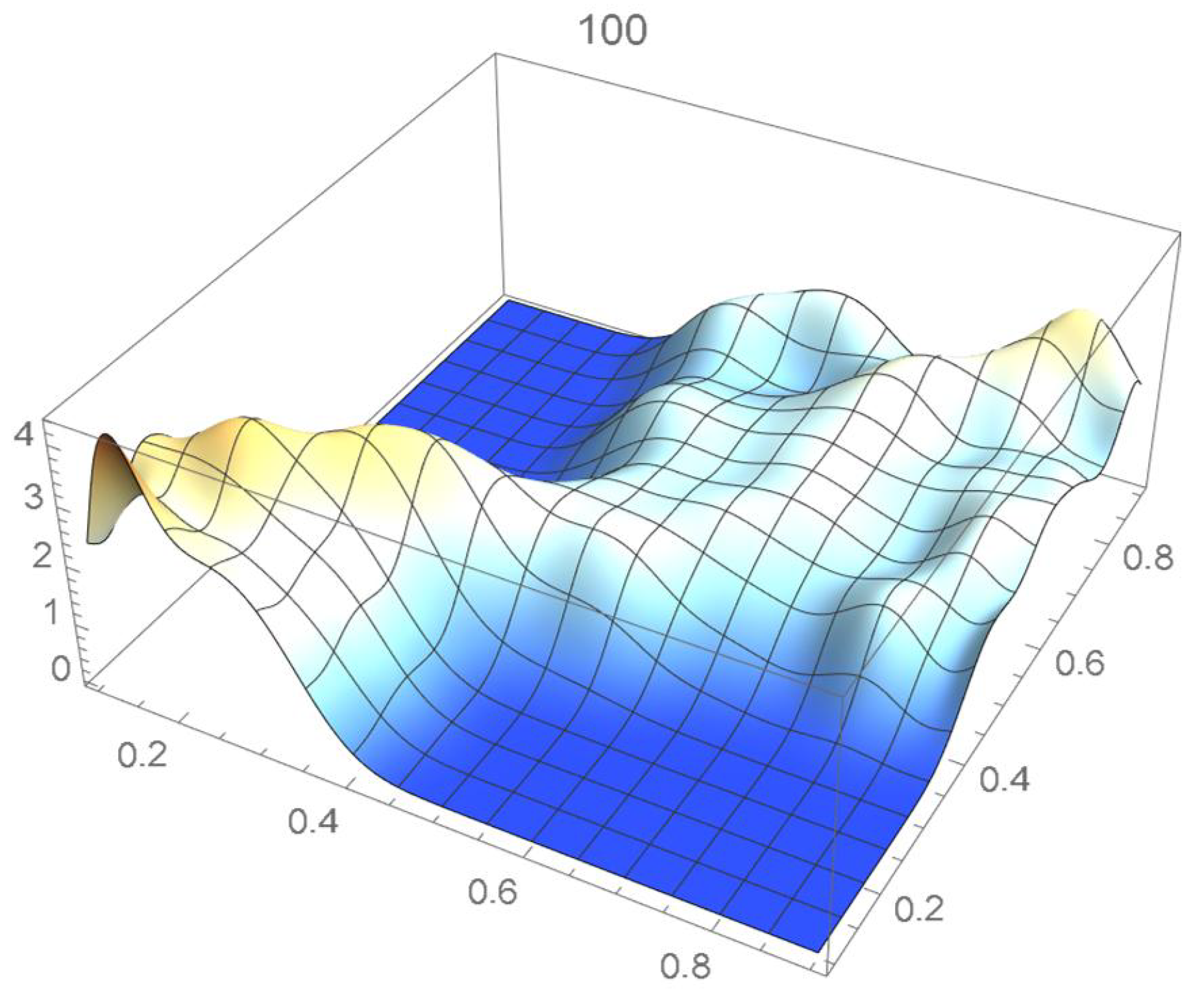
A kernel density estimate of the joint distribution is shown in Figure 14. The points , as defined in Equation (12), are plotted in Figure 15. A bivariate least-squares approximating polynomial of degree (in each variable) is fitted to the empirical copula points plotted in Figure 15 for , and differentiated with respect to each variable as explained in Section 2.1.1; finally, the resulting bivariate polynomial of degree t in each variable is normalized over the unit square. The copula density estimates so determined are plotted in Figure 16, Figure 17, Figure 18, Figure 19, Figure 20, Figure 21 and Figure 22. By mere visual inspection, one can observe that the copula density estimates of degrees 20, 25, 30, and 35 are analogous, while the estimate of degree 40 attains its maximum at a discernibly higher value than the previous estimates. Such a stable distributional behavior over an ample range of degrees—which incidentally are significantly lower that those required by the Bernstein polynomial approximations discussed in the next subsection—explains why the differentiated least-squares approach is discussed first and justifies employing the selected copula density estimate resulting from its use as the initial reference density.

Figure 14.
A bivariate kde.
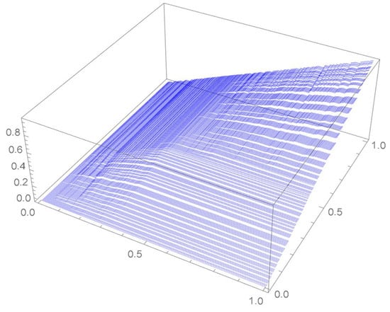
Figure 15.
The empirical copula.
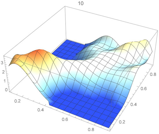
Figure 16.
Estimated copula pdf, .

Figure 17.
Estimated copula pdf, .

Figure 18.
Estimated copula pdf, .
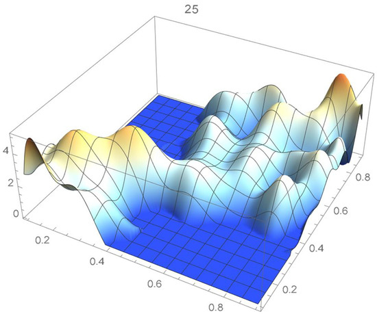
Figure 19.
Estimated copula pdf, .

Figure 20.
Estimated copula pdf, .

Figure 21.
Estimated copula pdf, .
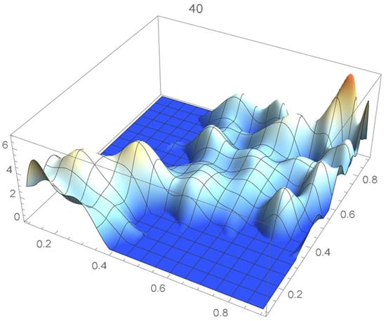
Figure 22.
Estimated copula pdf, .
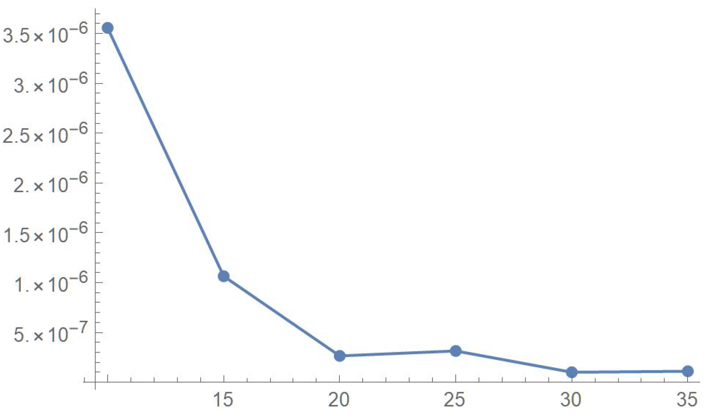
If smoothness is a key consideration, one ought to select the copula density of degree 20 in each of the variables as a yardstick for this copula distribution. This choice can be mathematically corroborated by noting that the integrated squared differences between successive copula estimates indicate that there is little to be gained by selecting copulas of degrees greater than 20, which can be inferred from the ISD’s listed in Table 1 and the graph shown in Figure 23. In actuality, the stability of the density estimates for such a wide array of degrees beyond 20 is indicative of their reliability.

Table 1.
ISD’s between successive density estimates that are five degrees apart.
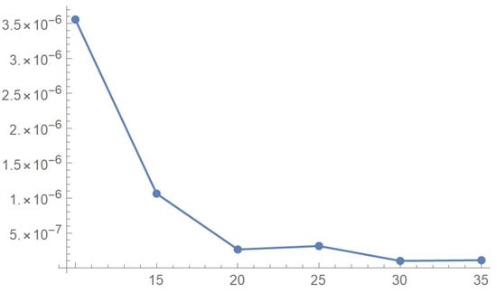
Figure 23.
ISD’s between successive least-squares copula estimates.
In this example, least-squares polynomial estimates are underfitting when as they do not adequately capture the distinctive distributional features of the copula, whereas estimates of degrees that are at least 20 in each variable turn out to be comparable up to degree 35. Beyond that degree, the estimates exhibit signs of overfitting. Thus, once normalized, the differentiated least-squares polynomial of order 20 in each variable is deemed to be a copula density estimate that is representative of the underlying copula distribution. A bona fide reference copula estimate can then be secured via integration.
2.2. Bernstein’s Copula Density and Degree Selection
2.2.1. Introduction
This section initially presents relevant background information on Bernstein’s empirical copula. A copula density function will be obtained by differentiating Bernstein’s polynomial approximation of Deheuvels’ empirical copula, and a criterion for determining a suitable degree for such an approximant, will be proposed. Leblanc [24] made use of Bernstein’s polynomials to estimate distribution functions that are defined on closed intervals, establishing their pointwise convergence. He also showed that such estimators are free of boundary bias.
First, we define Bernstein’s polynomials and describe some of their properties. A Bernstein polynomial of order k is obtained as follows:
where the ’s are called the Bernstein coefficients and is the Bernstein basis polynomial of degree k, which is also a binomial probability mass function when . The Bernstein basis polynomials have the following properties:
;
;
.
Moreover, their derivatives can be written as a combination of two polynomials of a lower degree:
The Bernstein approximating polynomial of a continuous function f on the interval is given by
It can be established that uniformly on the interval . This approximation approach can be generalized as follows to d dimensions. Letting be a continuous function on , can be approximated by the following Bernstein polynomial of order k in each variable:
Bernstein’s empirical copula was first introduced and investigated by Sancetta and Satchell [25] for identically and independently distributed (i.i.d.) data. Bernstein’s approximation of order k, , of a copula function C, the so-called Bernstein copula function, is defined as
for where k plays the role of bandwidth parameter and is the binomial probability mass function,
It has been shown that
In addition, under the conditions specified in Theorem 1 of Sancetta and Satchell [25], it was established that in (22) is itself a copula. Thus, in order to estimate the copula function , they proposed the following estimator referred to as Bernstein’s empirical copula:
where denotes the standard empirical copula estimator given by
where is the empirical cumulative distribution function of the component , and n is the sample size. Janssen et al. [26] demonstrated that Bernstein’s copula estimator outperforms the classical empirical copula estimator.
Whenever it exists, the copula density, denoted by , is obtained from the copula function as follows:
Since Bernstein’s copula function as specified in Equation (22) is absolutely continuous, Bernstein’s copula density can then be defined as
where is the derivative of with respect to . Accordingly, Sancetta and Satchell [25] proposed the following estimator of Bernstein’s copula density:
Later, Bouezmarni et al. [27] made use of Bernstein’s copula density to estimate the copula density in the presence of dependent data. More recently, Janssen et al. [28] established the asymptotic normality of this estimator given independently and identically distributed data.
In bivariate applications, the copula density given in (28) where the dimension d is two will be utilized, and the degree k of the copula density estimate will be taken to be such that there is no significant advantage in opting for a higher degree when compared to the selected least-squares copula.
2.2.2. An Illustrative Example
We are now estimating the copula density associated with the Old Faithful geyser eruption dataset by making use of Bernstein’s polynomial approximation technique.
The reference copula density function of degree 20 obtained in the previous subsection is shown in Figure 24, and Bernstein’s copula densities of degree 25, 50, 75, 100, 125, 150, and 200 are plotted in Figure 25, Figure 26, Figure 27, Figure 28, Figure 29, Figure 30 and Figure 31. The integrated squared differences (ISD’s) between Bernstein’s copula approximants, that are twenty-five degrees apart, and the reference copula are included in Table 2.
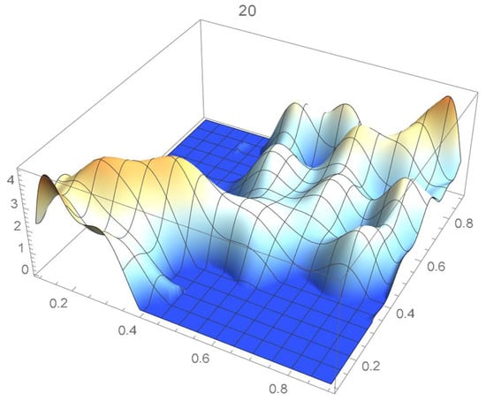
Figure 24.
Reference least-squares copula density of degree 20.
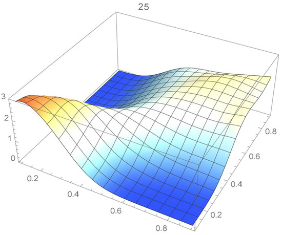
Figure 25.
Bernstein’s copula density of degree 25.

Figure 26.
Bernstein’s copula density of degree 50.
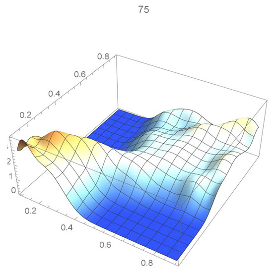
Figure 27.
Bernstein’s copula density of degree 75.

Figure 28.
Bernstein’s copula density of degree 100.

Figure 29.
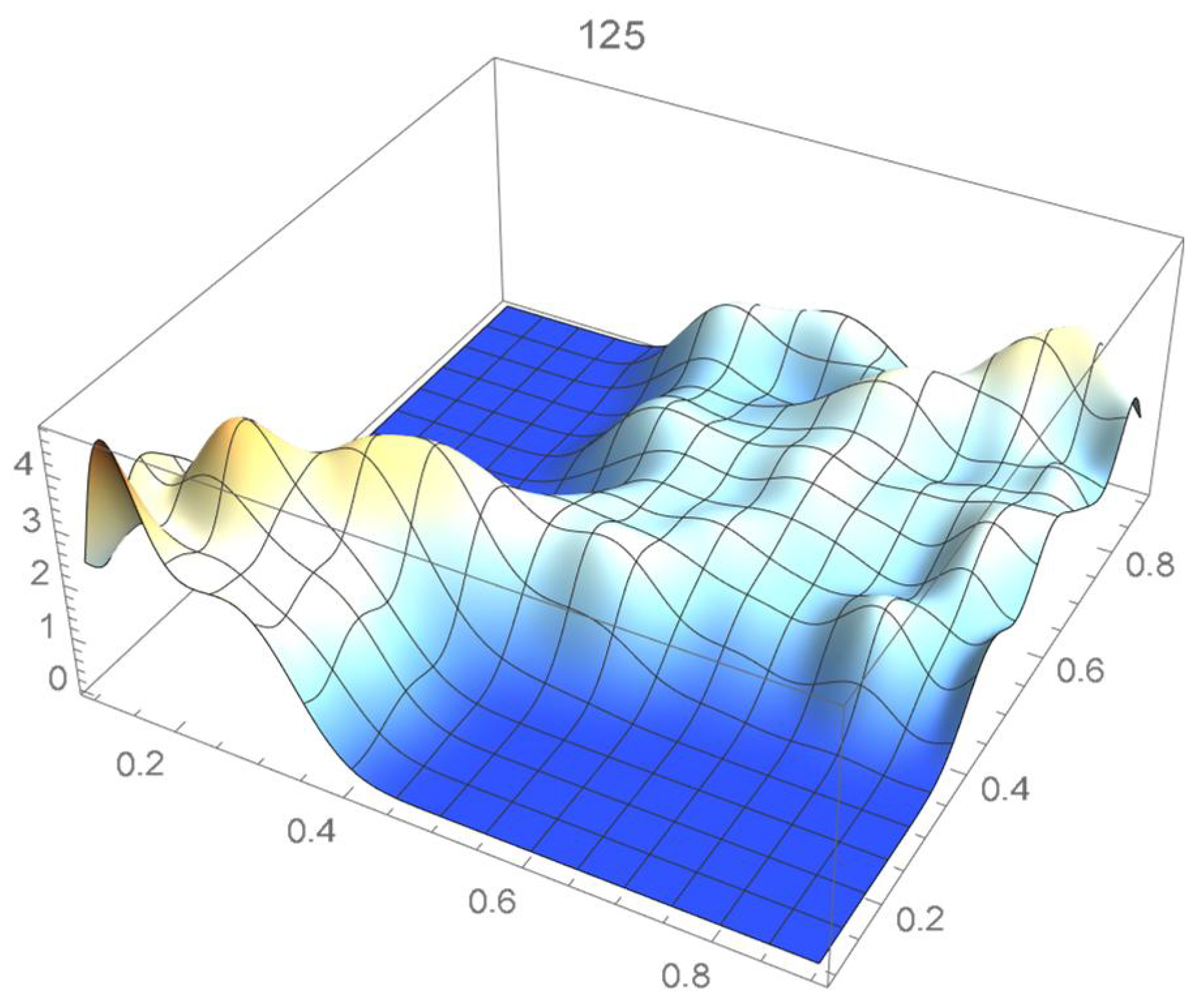
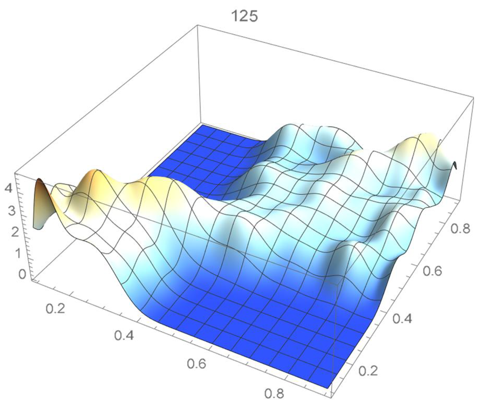
Bernstein’s copula density of degree 125.
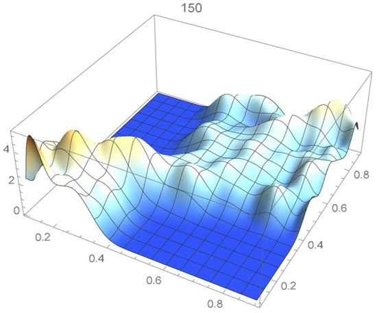
Figure 30.
Bernstein’s copula density of degree 150.

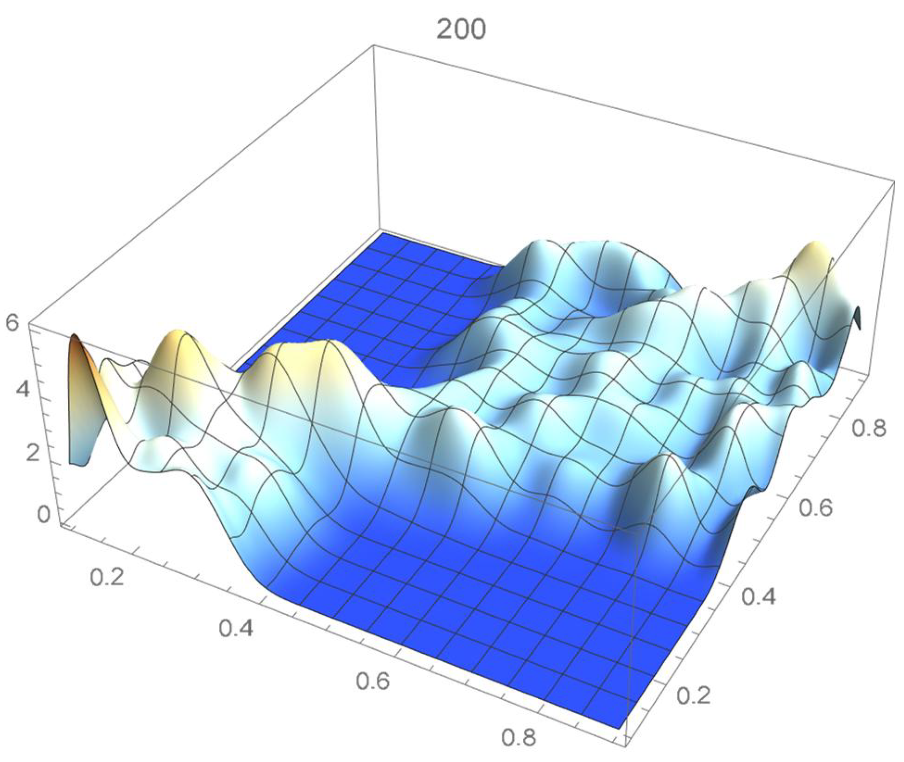
Figure 31.
Bernstein’s copula density of degree 200.
Table 2.
ISD’s between the reference copula and Bernstein’s’ for various degrees.
We observe that the ISD’s keep decreasing as the orders of Bernstein’s copulas keep increasing from 25 to 175. However, beyond degree 125, the ISD’s with respect to the selected least-squares copula turn out to be of the same order before they start increasing.
Accordingly, for the sake of parsimony, we may decide that Bernstein’s copula density of degree 125 in each variable is suitable, which is in agreement with the assessment resulting from a visual comparison with the selected least-squares density estimate. This density estimate will be utilized as the reference copula density in connection with the approaches that are presented in the two subsequent subsections. It should be noted that the Bernstein polynomial approximation technique readily produces bona fide copula density estimates.
2.3. Kernel-Based Copula Density Estimates
2.3.1. Introductory Considerations
Given a bivariate sample arising from a distribution whose density function is , a kernel density estimate is given by
where ; ; V is a bandwidth matrix assumed to be symmetric and positive definite; and , with the kernel being a bivariate density function such as the standard bivariate Gaussian density function. For additional considerations on bivariate kernel density estimation, the reader is referred to Duong and Hazelton [29], Sheater and Jones [30], and Wand and Jones [31], among others.
For instance, Li and Silvapulle [32], Geenens et al. [33], and Wen and Wu [34] employed kernel density estimates (kde’s) in the context of copula density estimation. Since the support of copulas is finite, kde’s can produce what is referred to as ‘boundary bias’. Gijbels and Mielniczuk [35] attempted to address this drawback by making use of a certain mirror reflexion methodology. It will be explained that boundary effects can be alleviated as well by repositioning the usual pseudo-observations and making use of kernels having a finite support.
For illustrative purposes, let the pseudo-observations be . It will be shown that, as explained in Section 1.3, centering them within grid cells can significantly alleviate the boundary issues associated with the original pseudo-observations in the context of kernel density estimation. Bi-weight kernels whose density function is are utilized in this example. The resulting kde’s of the copula density, as secured from the original and centered pseuso-observations, are plotted in Figure 32 and Figure 33. The corresponding copulas, which were obtained via integration, are shown in Figure 34 and Figure 35.
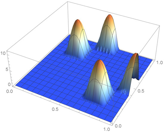
Figure 32.
kde obtained from the original pseudo-observations.
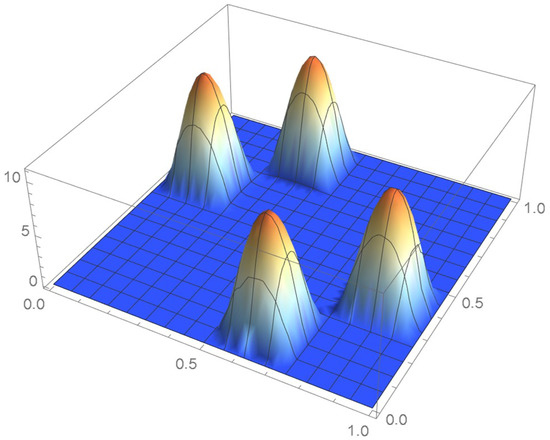
Figure 33.
kde obtained from the centered pseudo-observations.

Figure 34.
Copula resulting from the original pseudo-observations.
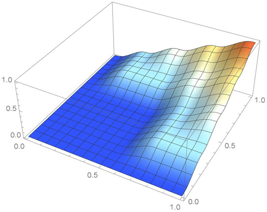
Figure 35.
Copula resulting from the centered pseudo-observations.
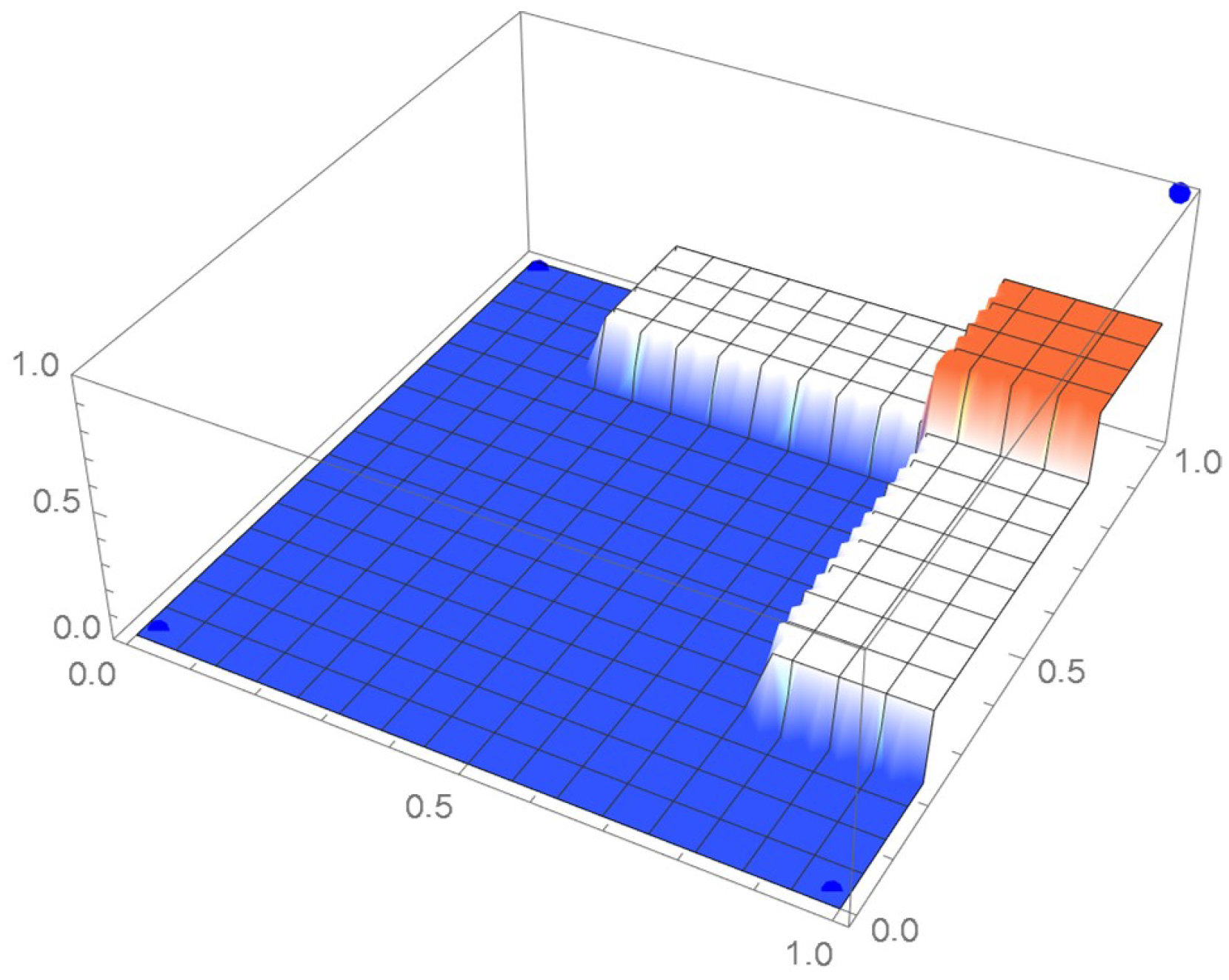
It is seen that two of the kernels centered at the original pseudo-observations are truncated. Moreover, as the graph of the cumulative distribution function indicates, the resulting kde integrates to less than 0.8 over the unit square whereas, in this case, the cumulative distribution function tends to one when the centered pseudo-observations are utilized. Actually, a kde will never integrate to one within the unit square when the selected kernel is centered at each of the usual pseudo-observations or defined on an infinite support. In the current context, it is thus advisable to make use of finite-support kernels whose modes occur at the centered pseudo-observations.
2.3.2. Kernel Bandwidth Selection
A mathematical criterion for selecting an appropriate kernel bandwidth is proposed in this subsection. As centered pseudo-observations yield improved copula density functions, kde’s of various bandwidths, which are centered at those points, are initially obtained and then compared to a reliable reference copula density, such as the selected Bernstein or least-squares copula density functions.
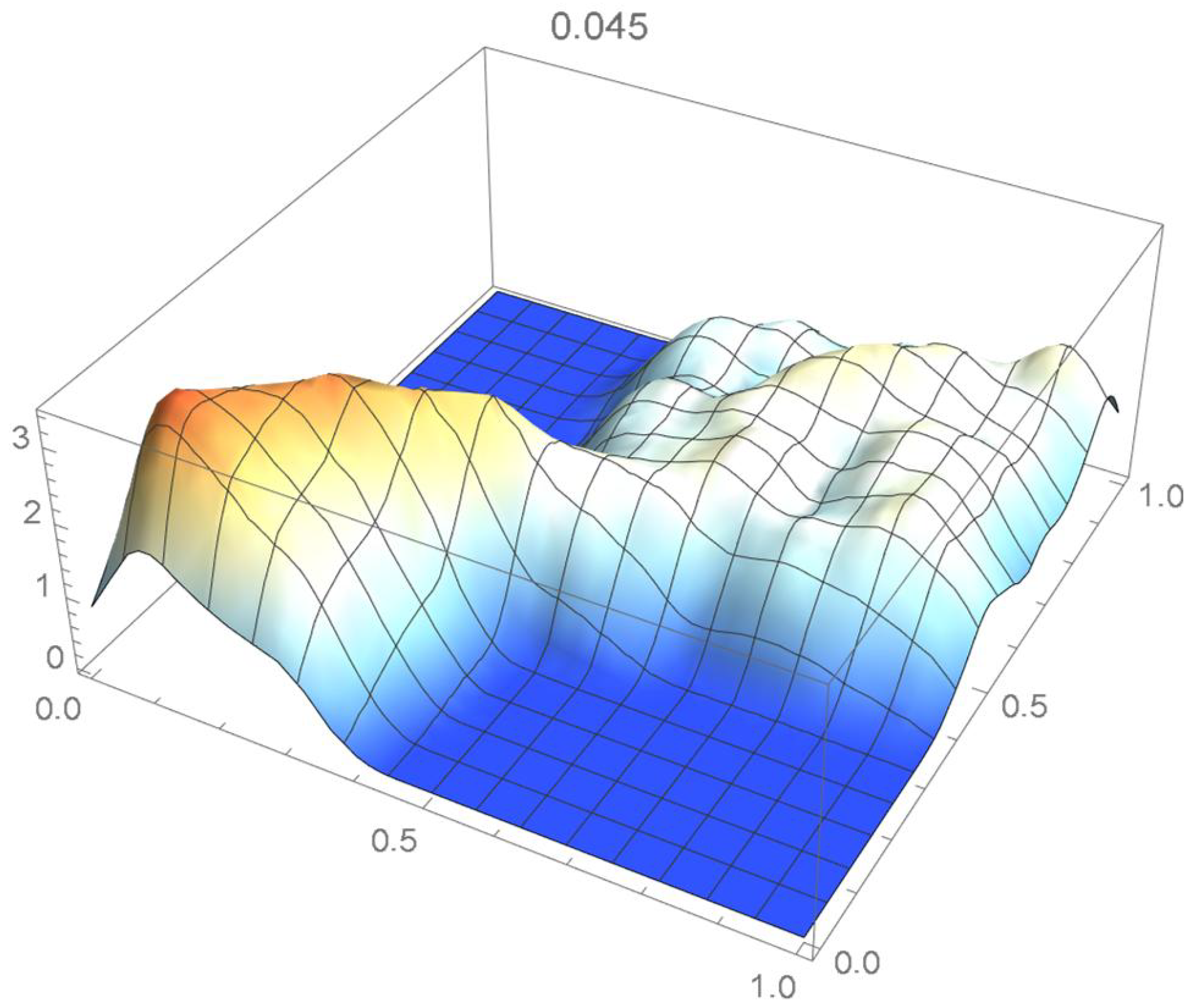
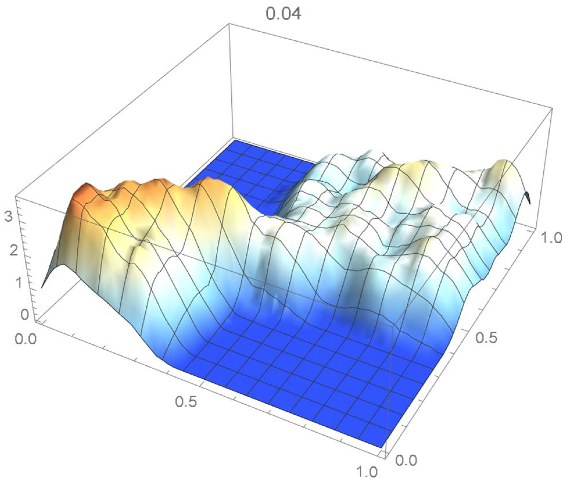
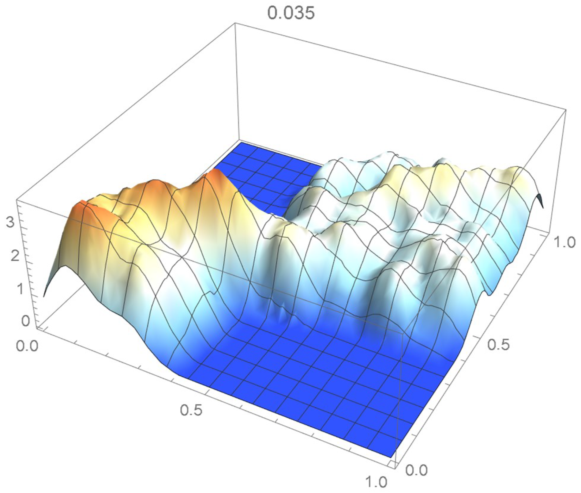
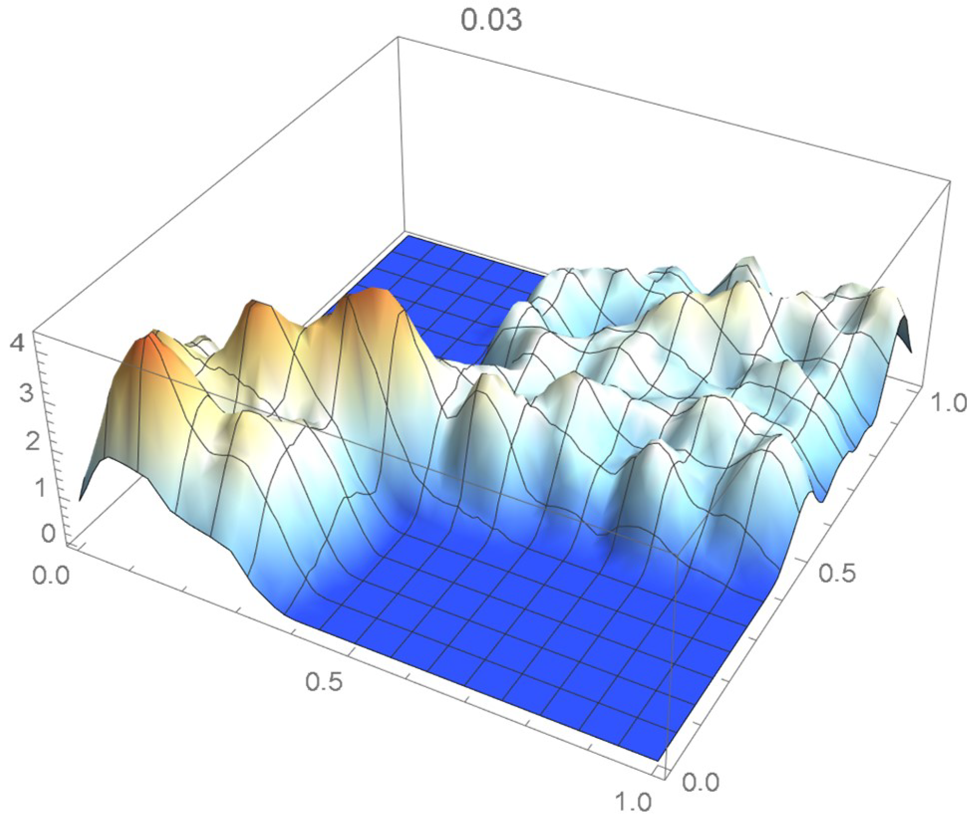
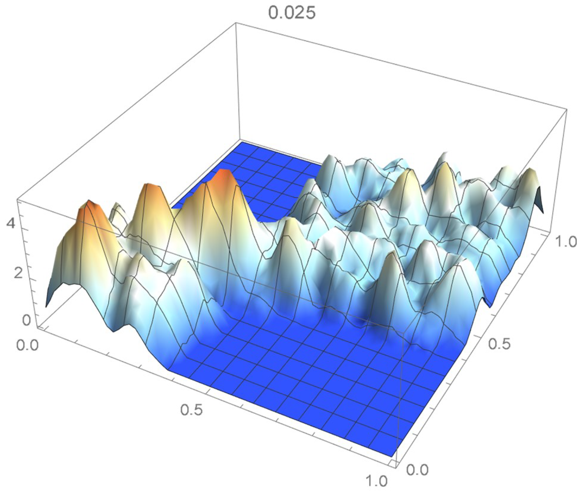
Once again, we rely on the Old Faithful geyser eruption observations for illustrative purposes. In this instance, the selection criterion will be based on the integrated squared difference between the selected Bernstein copula density shown in Figure 36 and Epanechnikov kde’s of bandwidths 0.045, 0.04, 0.035, 0.030, and 0.025, which are plotted in Figure 37, Figure 38, Figure 39, Figure 40 and Figure 41.

Figure 36.
Bernstein’s copula density of degree 125.

Figure 37.
kde with a bandwidth of 0.045.

Figure 38.
kde with a bandwidth of 0.040.

Figure 39.
kde with a bandwidth of 0.035.

Figure 40.
kde with a bandwidth of 0.030.

Figure 41.
kde with a bandwidth of 0.025.
It is seen from the ISD’s listed in Table 3 that the smallest ISD corresponds to a bandwidth of 0.035. Accordingly, the copula kde having this bandwidth is selected as being the most suitable one, a conclusion that, incidentally, could also have been reached via visual inspection.
Table 3.
ISD’s between the reference copula density and kde’s of various bandwidths.
2.4. Differentiated Linearized Empirical Copulas
2.4.1. Methodology and Implementation
A novel approach to copula density estimation is described in this subsection. A Deheuvels’ empirical copula is first determined for the dataset at hand by making use of Equation (12). Next, the empirical copula is evaluated at grid points of the unit square whose associated spacing along both directions is denoted by c. Then, linear interpolation is applied to those points within each grid cell and the resulting surface is differentiated, which yields an approximate density function. As the resulting copula density is obtained by differentiating a linearized copula, it will be referred to as a copula density. The spacing parameter c is chosen in such a way that the copula density function and a reference copula density—for instance, the selected Bernstein polynomial approximation—share similar distributional features. Mathematically, c is taken to be the minimizer of the integrated squared difference between the chosen reference copula density and differentiated linearized copula densities resulting from various values of the spacing parameter.
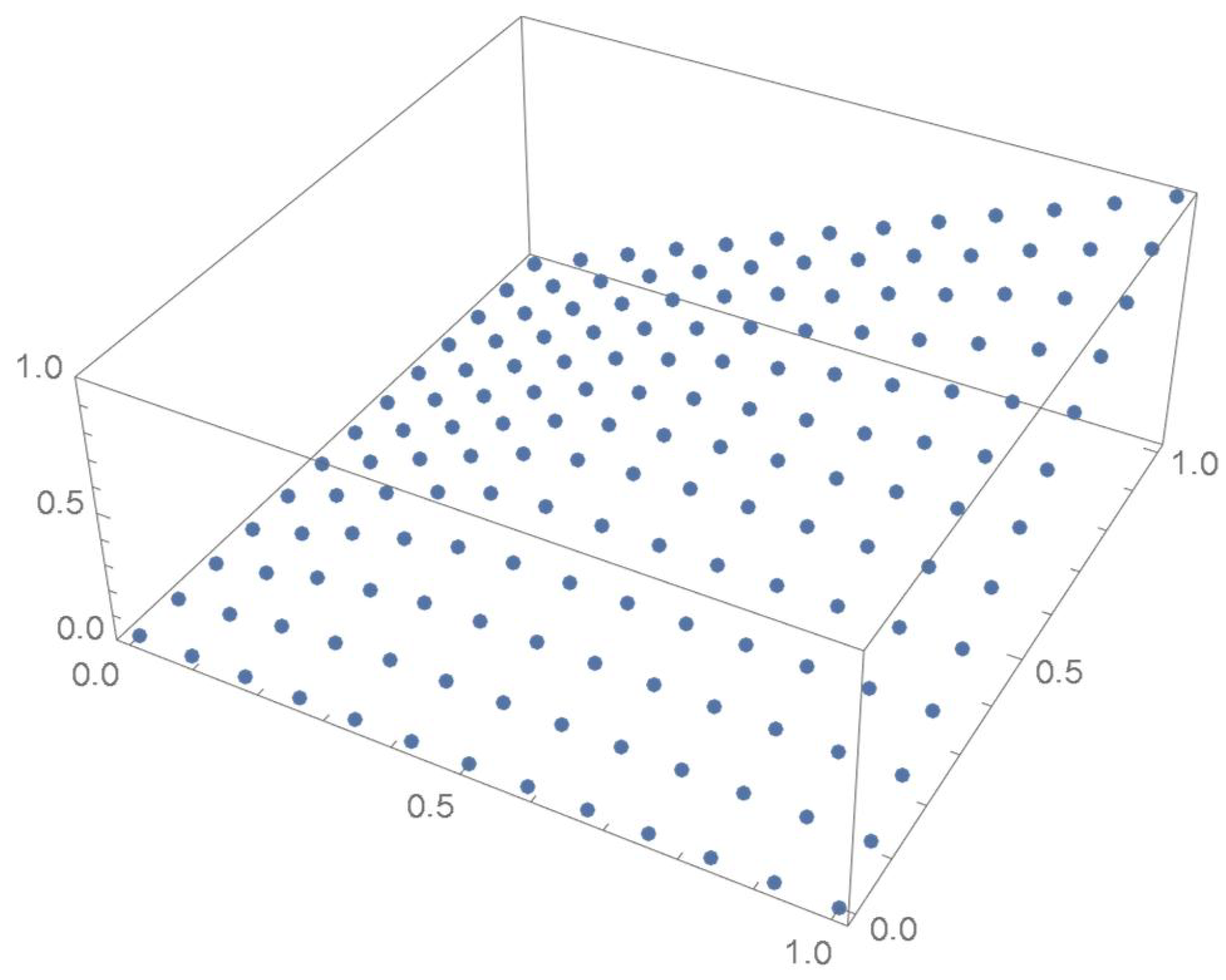
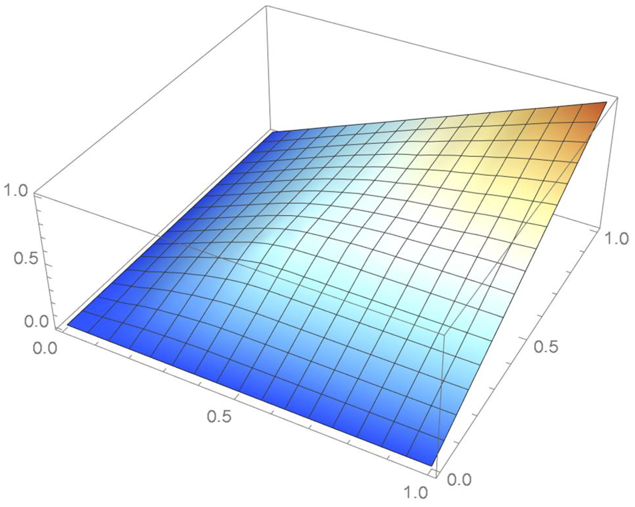
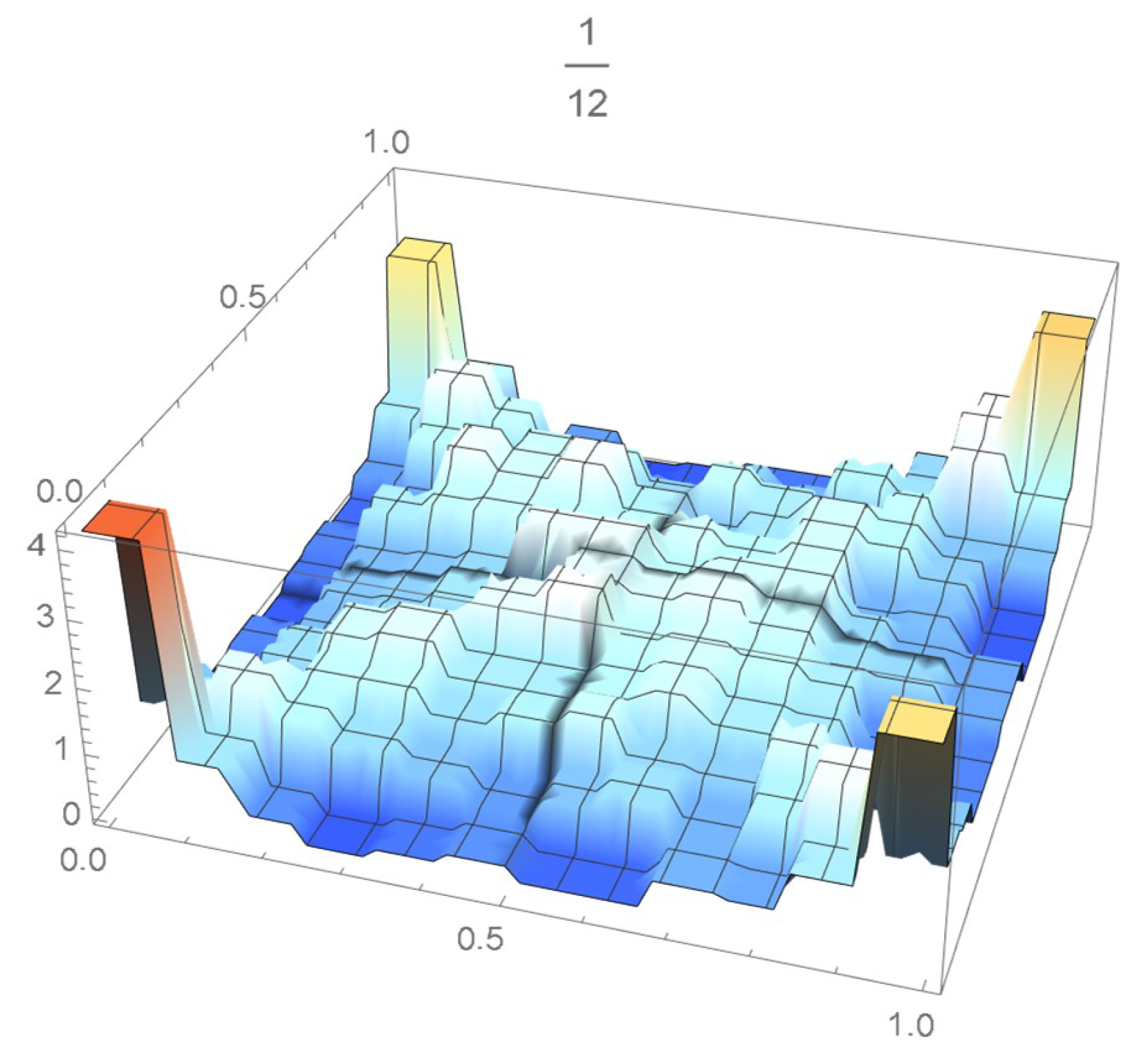
The grid points of the empirical copula as determined from the Old Faithful geyser dataset, which are plotted in Figure 42, are apart. Linear interpolation was applied within each grid cell. The resulting linearized copula and copula density obtained via differentiation are respectively plotted in Figure 43 and Figure 44. As Table 4 indicates, the appropriate spacing parameter c is 1/12 in this case. For comparison purposes, the copula density functions are also plotted for and in Figure 45 and Figure 46.

Figure 42.
Empirical copula at grid points that are 1/12 apart.
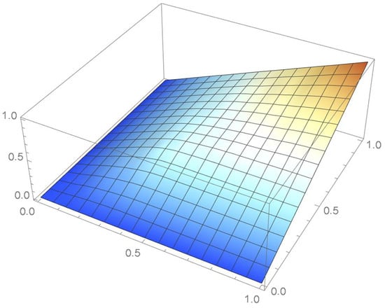
Figure 43.
The resulting linearly interpolated surface.
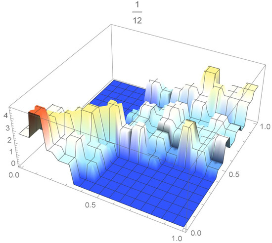
Figure 44.
copula density with spacing parameter .
Table 4.
ISD’s between the reference copula density and certain copula densities.
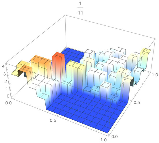
Figure 45.
copula density with spacing parameter .
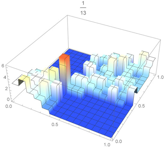
Figure 46.
copula density with spacing parameter .
2.4.2. Smoothing a Copula Density Estimate by Means of a Polynomial
The selected copula density that is plotted in Figure 44 was smoothed by approximating it with an eleventh degree moment-based bivariate polynomial—as defined in Result 2. The resulting bona fide density function that was obtained after normalization is shown in Figure 47. In this instance, the base density was taken to be the uniform distribution.

Figure 47.
Bivariate polynomial approximation of the selected copula density.
2.5. Estimating Joint Density Functions by Means of Copula Density Estimates
2.5.1. Introduction
The following formula, which can be deduced from Result 1 (Sklar’s theorem), expresses a joint density function estimate in terms of estimates of the marginal density and distribution functions and a copula density estimate denoted by :
Thus, once a copula density estimate has been secured, it is a rather simple matter to obtain a joint density estimate. More specifically, one would proceed as follows: First, the marginal density functions and associated with the random variables X and Y are estimated and their respective distribution functions are obtained via integration; then, a copula density estimate is determined by implementing one of the proposed methodologies, and a joint density estimate is secured by making use of the representation given in Equation (29). This alternative approach to determining joint density function estimates allows for more flexibility than the direct approach. For instance, one has then the option to rely on some prior information for selecting appropriate tuning parameters—such as degrees or bandwidths—for each of the marginal density functions and for assigning a suitable degree of smoothness to the copula density estimate.
2.5.2. An Illustrative Example
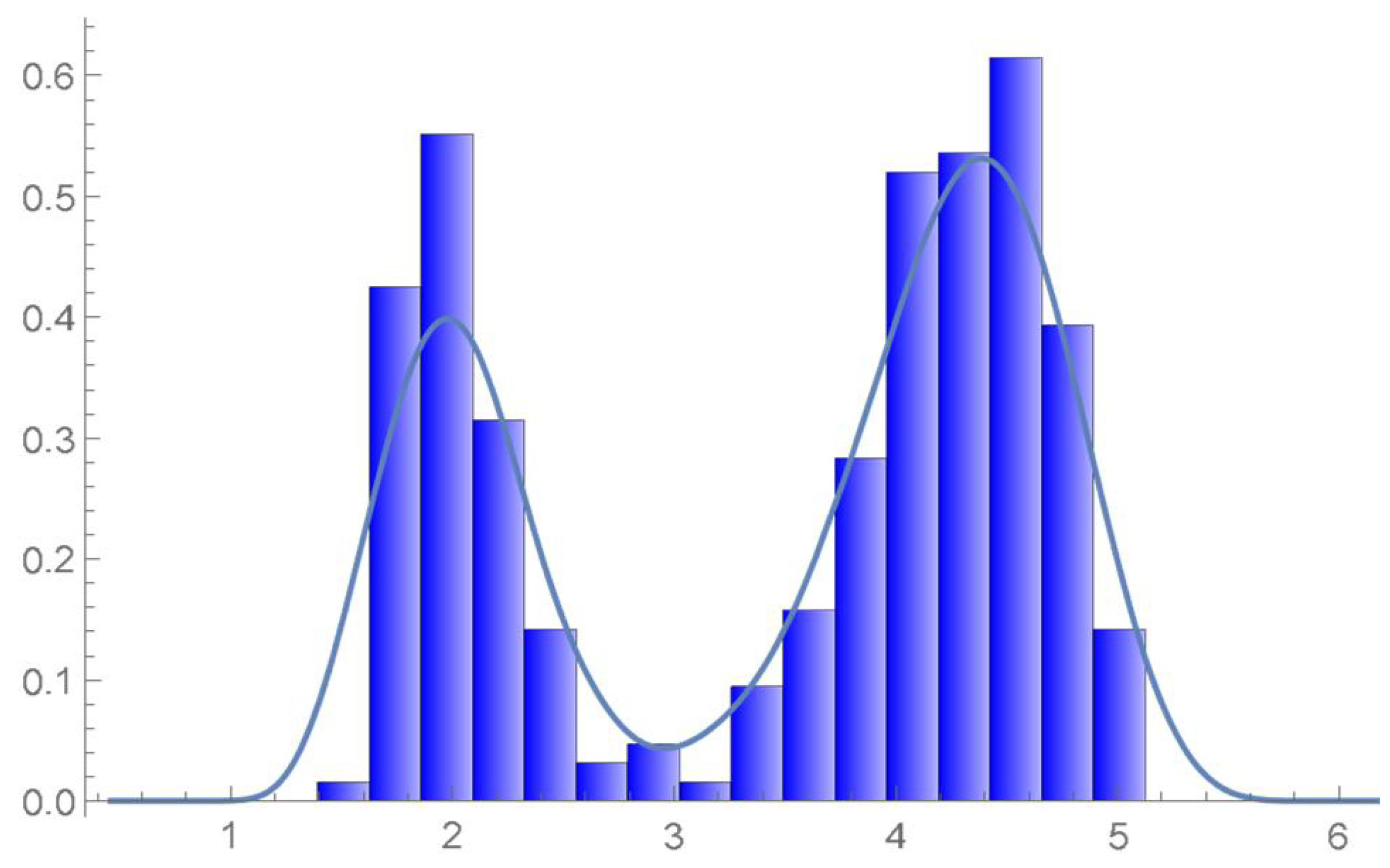
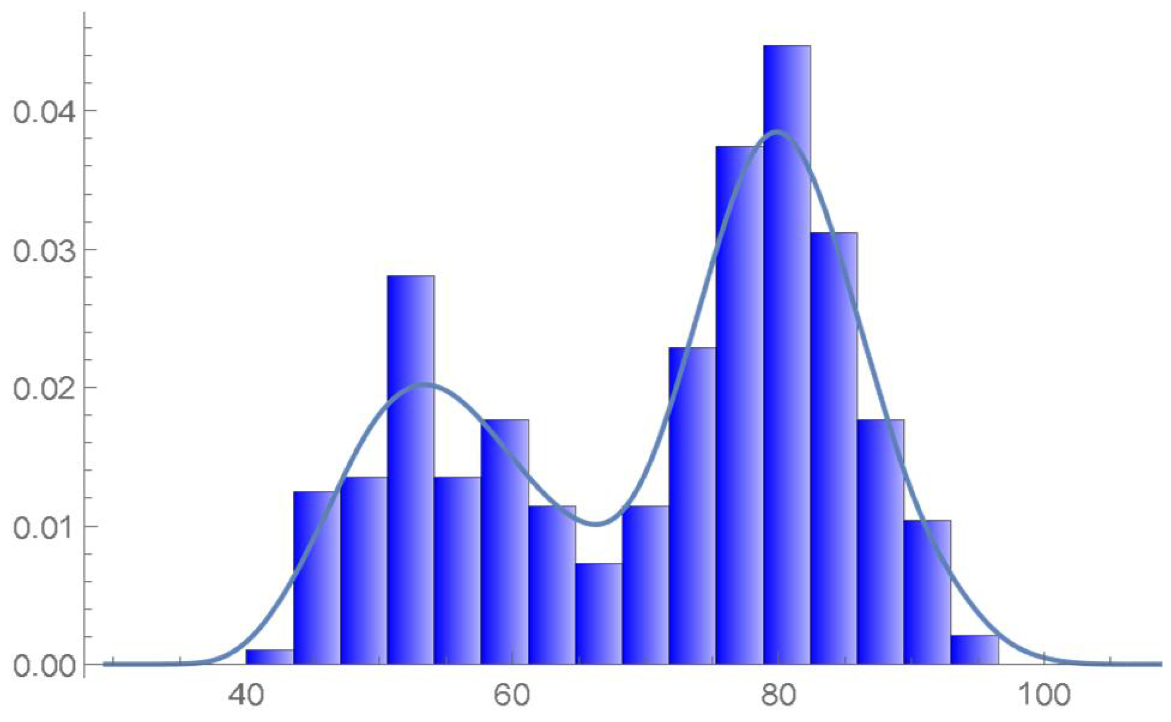
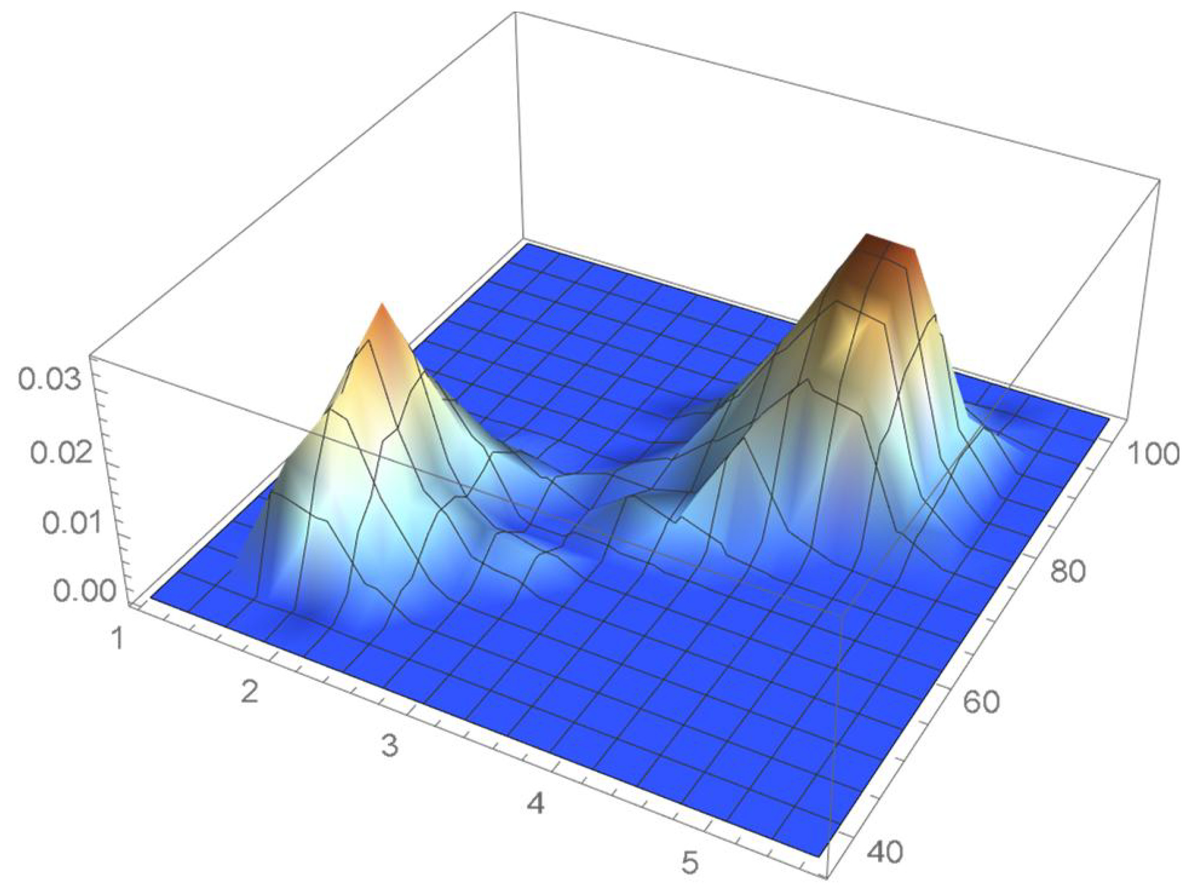
Consider once again the Old Faithful geyser eruption data. A kde of the copula density whose suitable bandwidth was determined to be 0.035 is plotted in Figure 48. Kernel density estimates of the marginal density functions are superimposed on histograms of the observations on each of the variables in Figure 49 and Figure 50. It is seen that the bivariate kde shown in Figure 51, which was secured directly from the data, and the estimated joint density obtained from Equation (29), which appears in Figure 52, exhibit similar features.
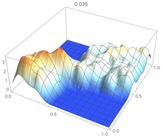
Figure 48.
Copula kde with a bandwidth of 0.035.
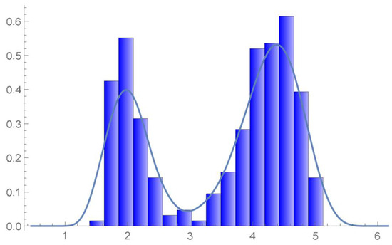
Figure 49.
The estimated marginal density of the first variable and histogram.

Figure 50.
The estimated marginal density of the second variable and histogram.

Figure 51.
Bivariate kde obtained directly from the observations.
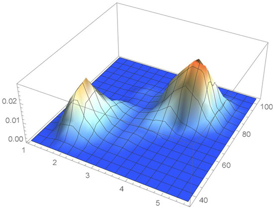
Figure 52.
Joint density estimate resulting from applying Sklar’s theorem.
3. Estimating a -Distributed Copula Density
3.1. Introduction
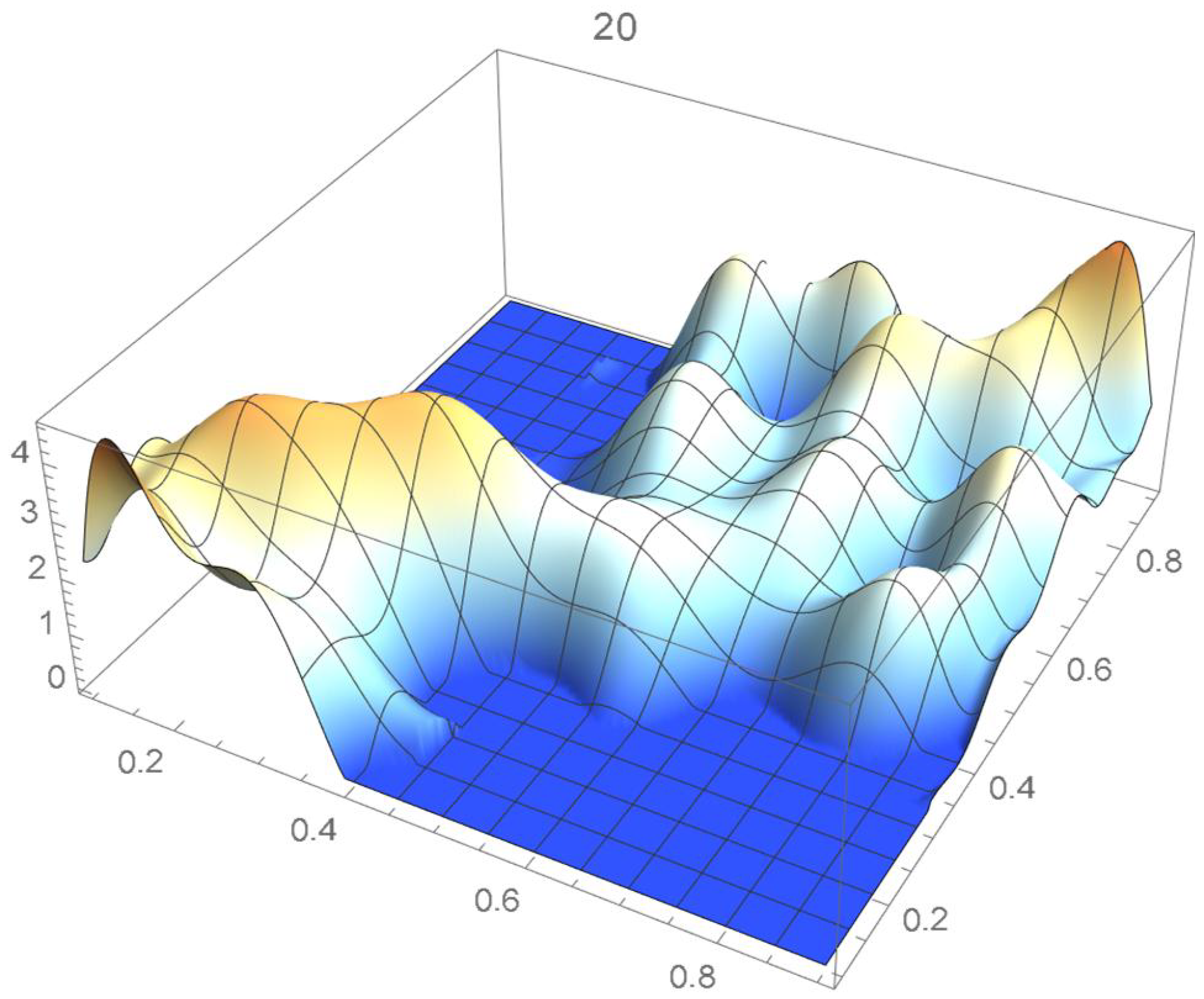
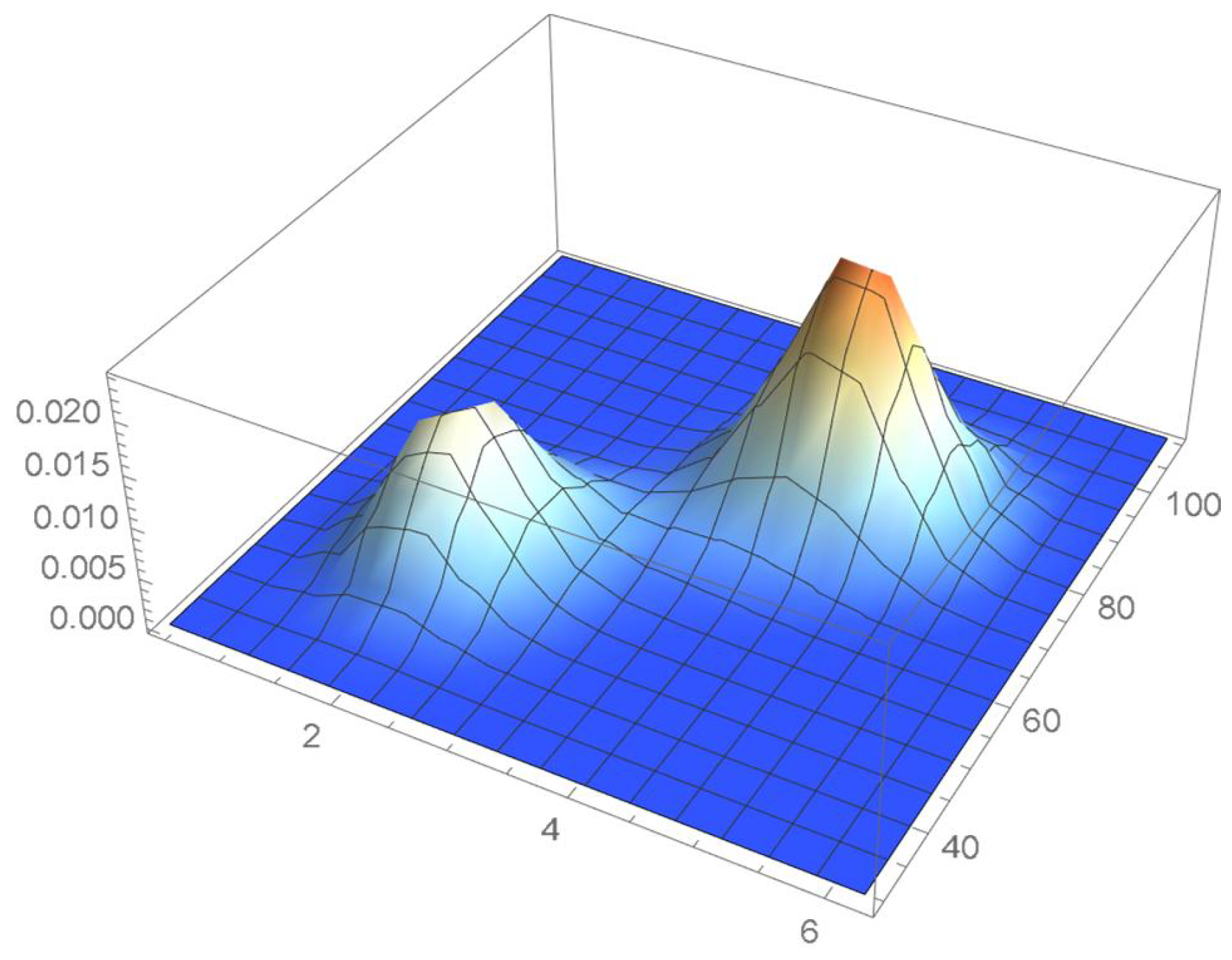
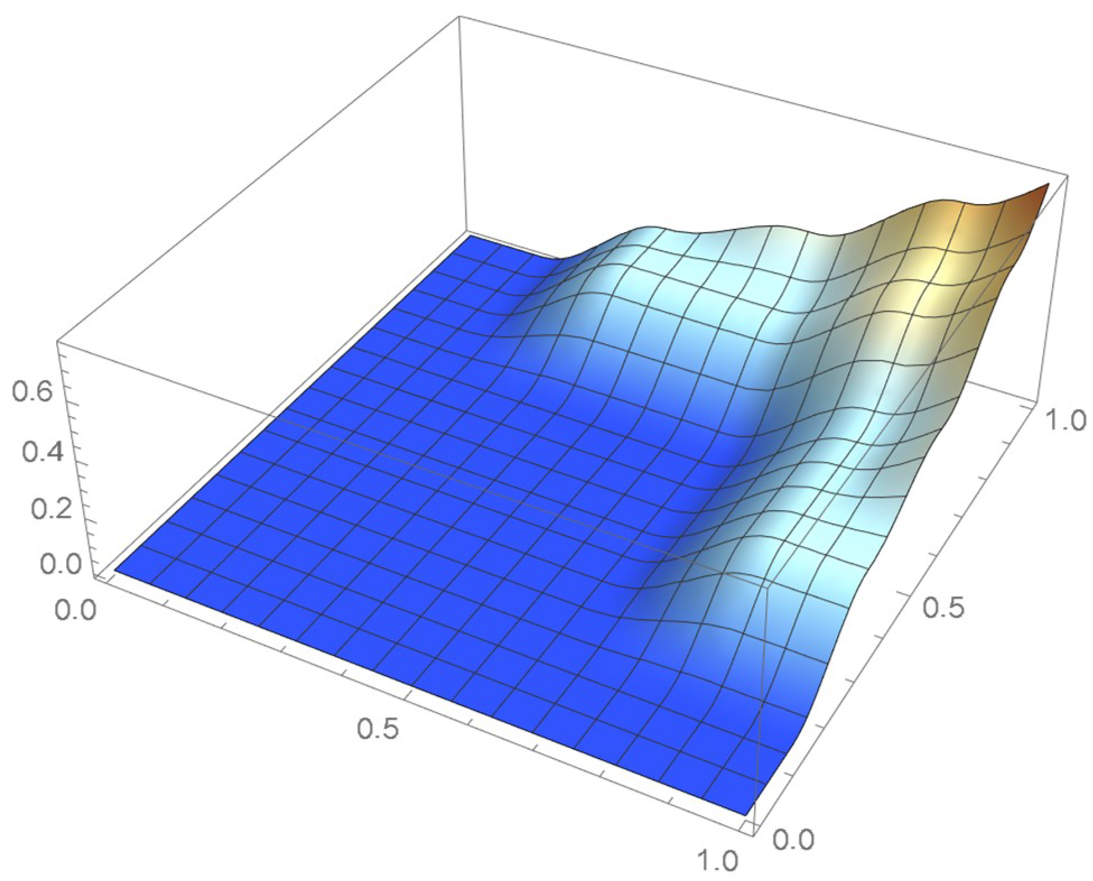
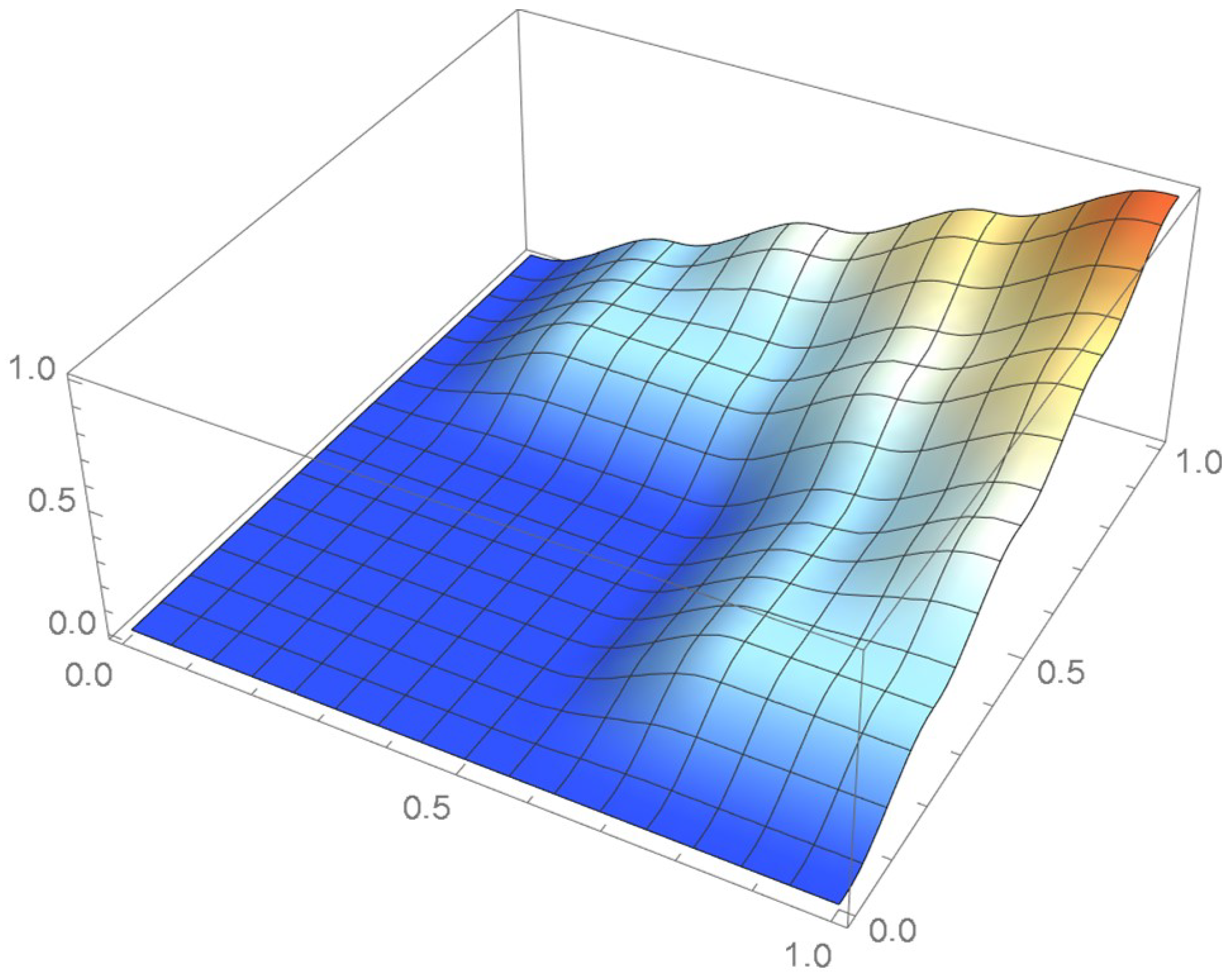
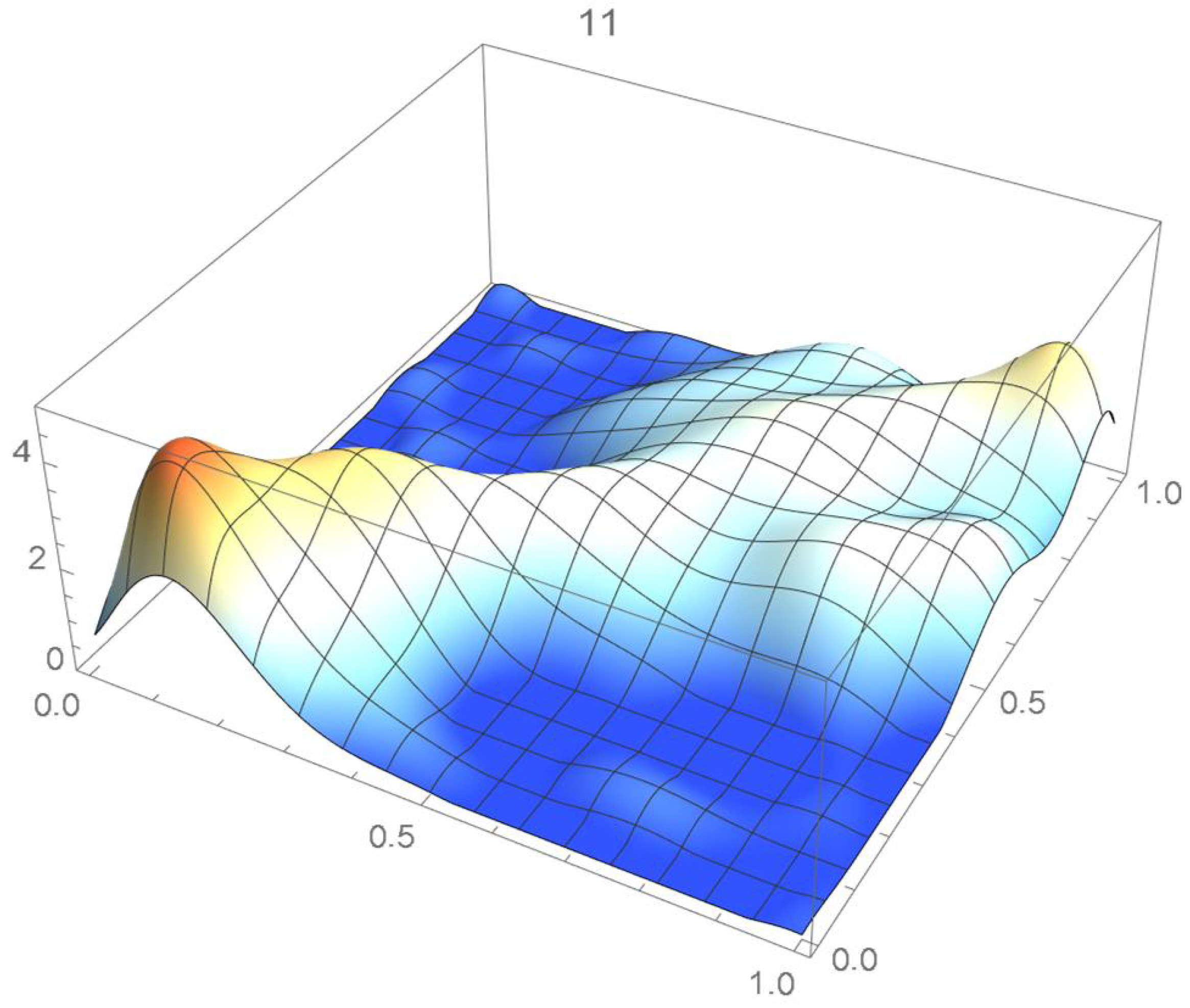
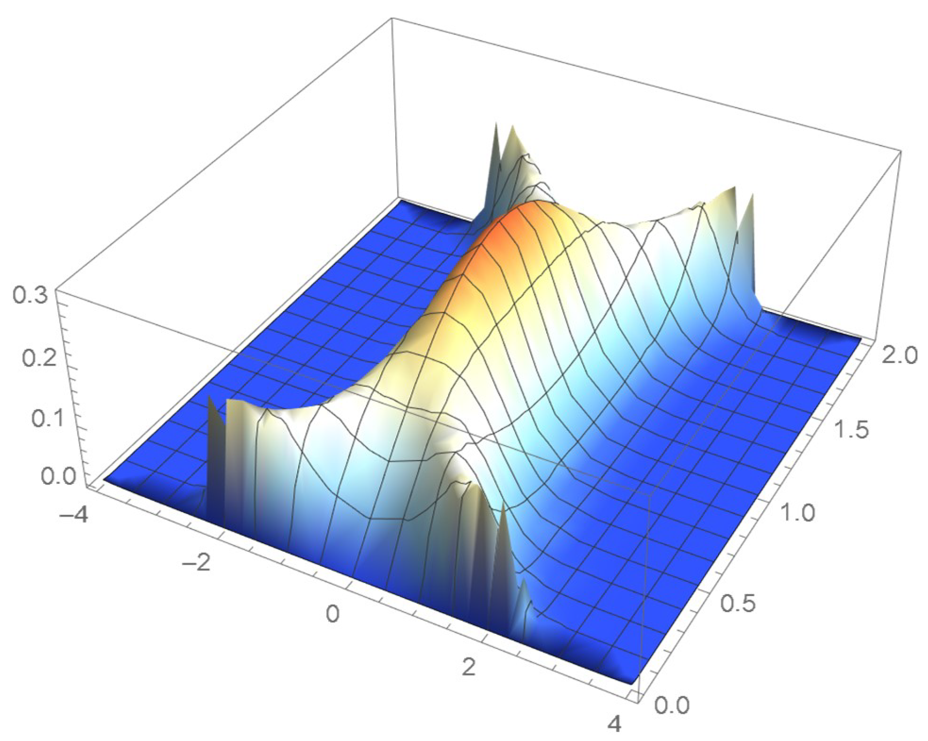
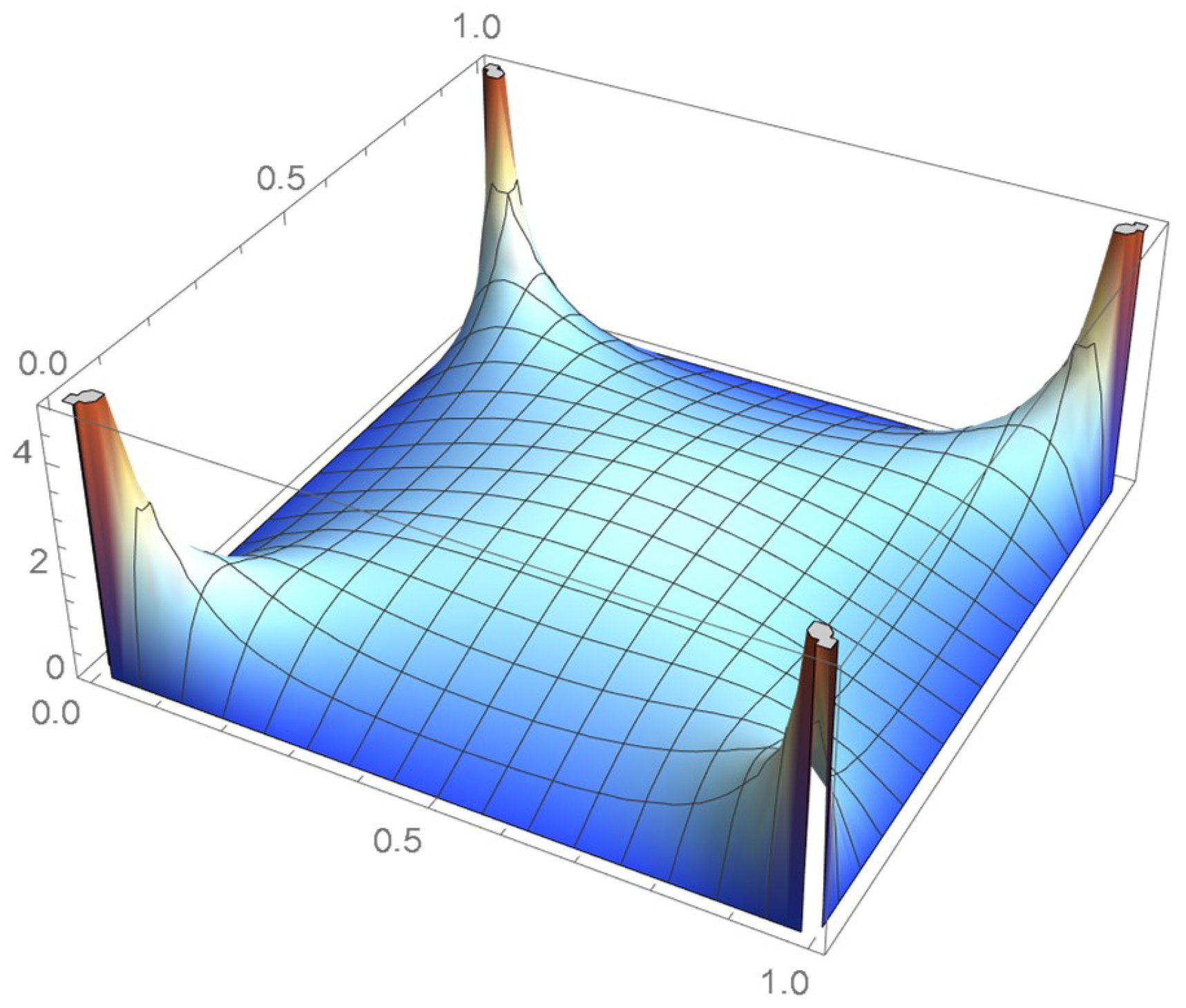
The four density estimation techniques introduced in Section 2 are applied to a random sample of size 2000 that was generated from a distribution whose associated copula is distributed as a bivariate Student’s t on only one degree of freedom, the marginal distributions being respectively standard normal and uniform on the interval . It should be noted that the selected copula proves challenging to model as its density function tends to plus infinity at each of the four vertices of the unit square. Moreover, as pointed out in Quintero et al. [1], heavy-tailed distributions are generally more difficult to model. The exact joint and copula density functions are respectively plotted in Figure 53 and Figure 54.

Figure 53.
The joint density function.
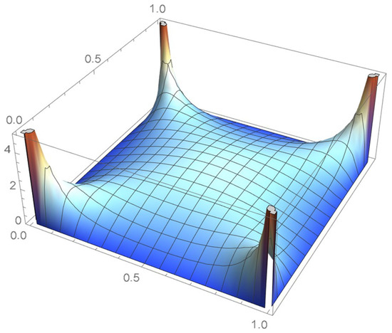
Figure 54.
The bivariate Student’s t copula density on one degree of freedom.
3.2. Application of the Proposed Methodologies
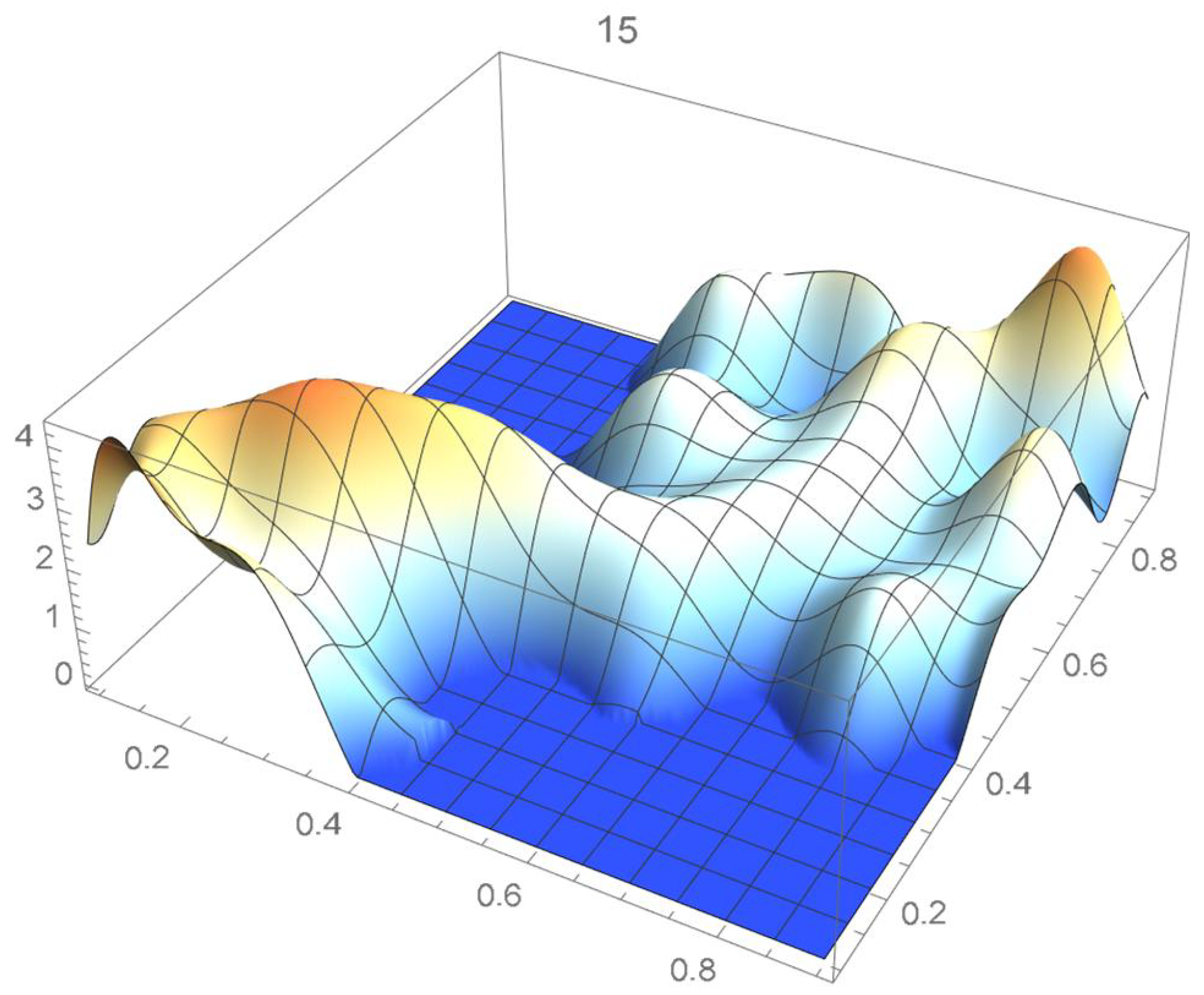
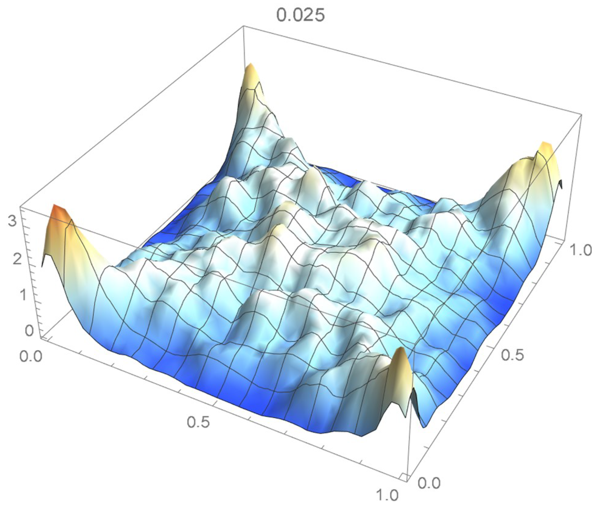
Proceeding as explained in Section 2.1, it was determined that a suitable degree for the differentiated least-squares bivariate polynomial approximation is 30. The resulting copula density estimate is plotted in Figure 55. On following the methodology advocated in Section 2.3.2, it was found that the kde-based estimate having 0.025 as its bandwidth, shown in Figure 56, is appropriate.
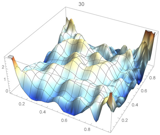
Figure 55.
Differentiated least-squares density estimate of degree 30.

Figure 56.
A kde whose bandwidth is 0.025.
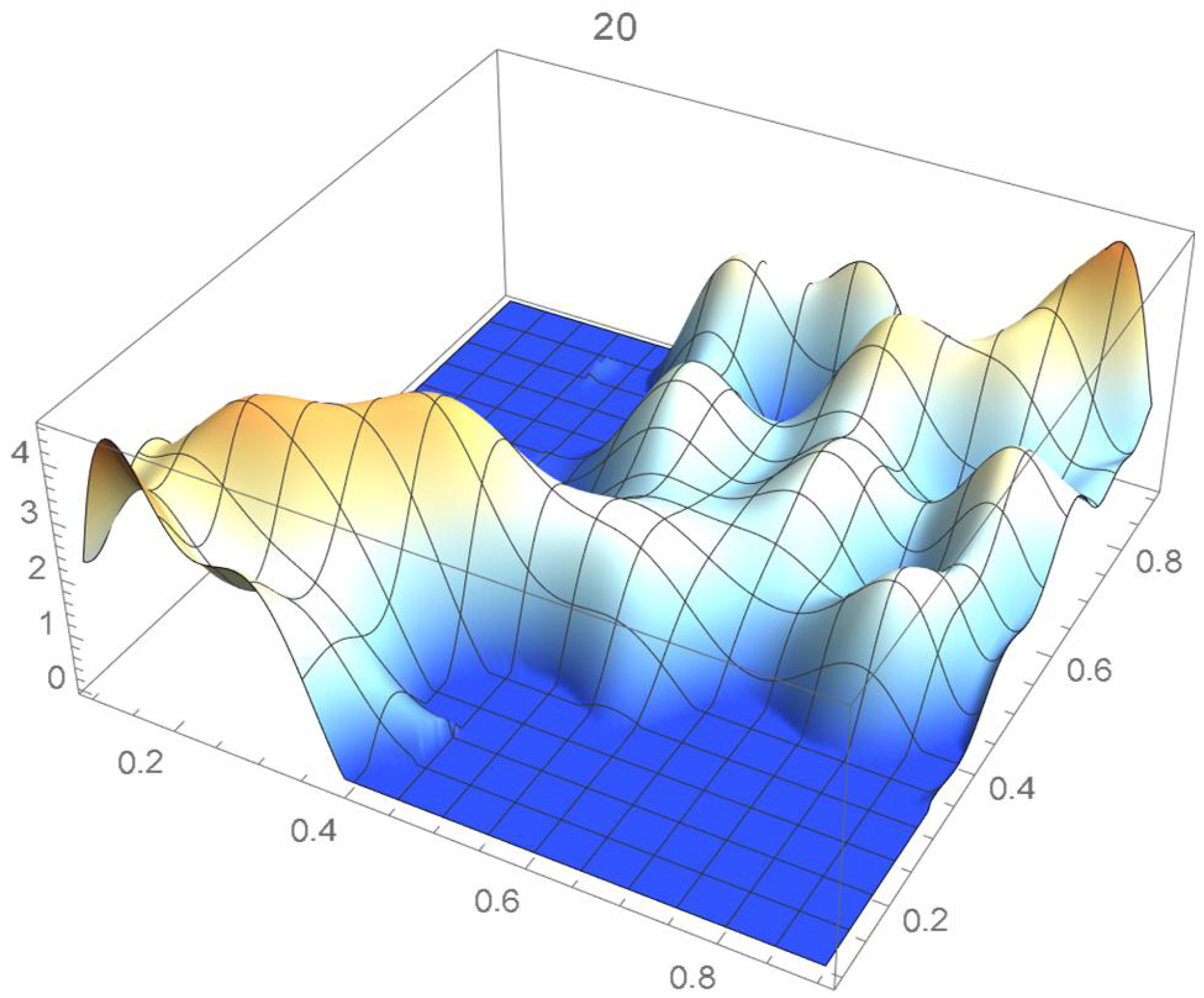
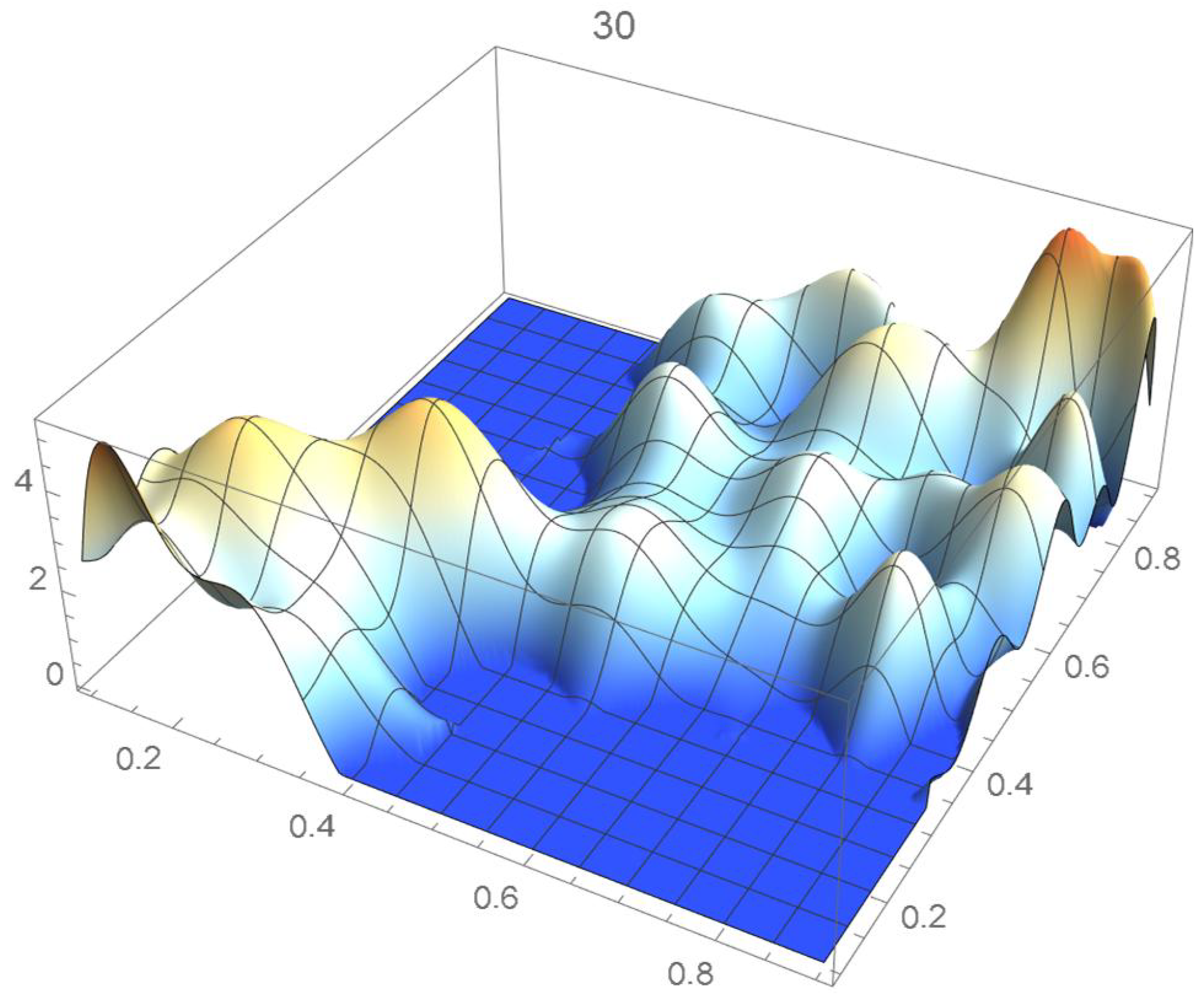
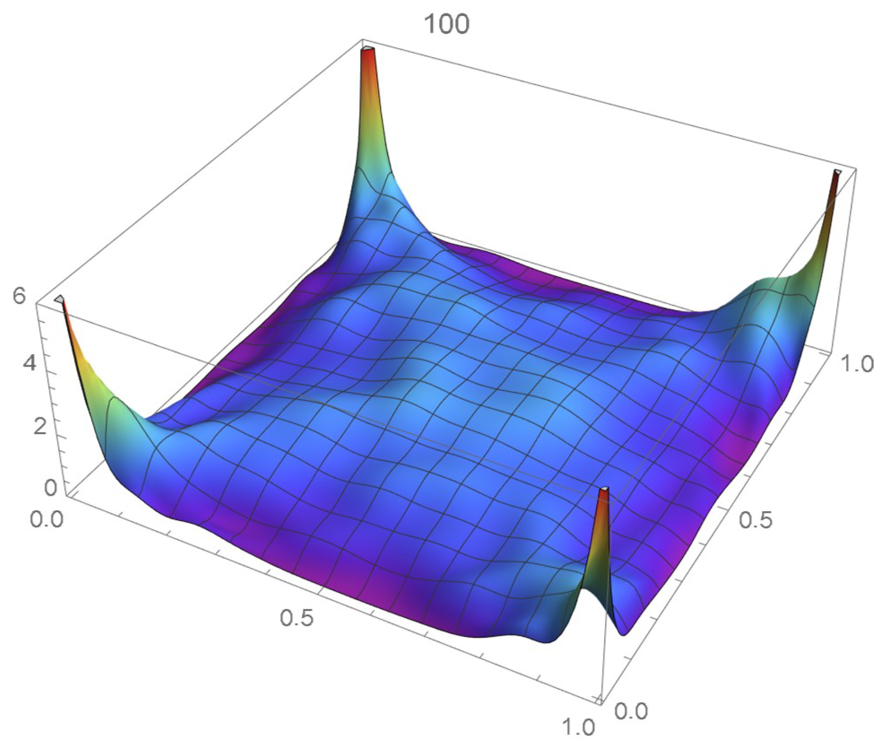
Referring to Section 2.2, it was determined that an appropriate degree for Bernstein’s copula density estimate is 100. This density function is plotted in Figure 57. Now, proceeding as explained in Section 2.4, the proper spacing for the copula density was determined to be . This copula density is shown in Figure 58.

Figure 57.
Bernstein’s copula density of degree 100.

Figure 58.
copula density obtained with 1/12 as spacing parameter.
All of these density estimates exhibit distributional features that are consistent with those of the underlying distribution, which supports the validity of the various methodologies being advocated in this paper.
3.3. Identification of the Underlying Distribution
For illustration purposes, we assess whether the distribution of a previously determined Student’s t copula density estimate can be correctly identified when compared to several parametric copula density functions by making use of the Hellinger distance measure, which constitutes an alternative to the Kullback–Leibler divergence for comparing density or distribution functions. Another distance measure is studied in Fournier and Guillin [36].
If we denote the probability density functions of two bivariate distributions as and , the square of the Hellinger distance between them is given by
The Hellinger distances between Bernstein’s copula density approximation of degree 100, which is plotted in Figure 57, and the following copula density functions were evaluated: bivariate Student’s t on 1, 3, and 10 degrees of freedom; bivariate Gaussian; Farlie–Gumbel–Morgenstern; Ali–Mikhail–Haq; Gumbel–Hougaard; Frank; and Clayton–Pareto. In this instance, the lower and upper bounds of integration are zero and one in Equation (30).
As anticipated, the Hellinger distance between the estimated copula density and the bivariate t copula density on one degree of freedom turned out to be the smallest.
4. Concluding Remarks
Four types of nonparametric copula density estimates were considered and criteria for selecting their tuning parameters were proposed. Bernstein’s polynomial density estimates enjoy the advantage of not having to be normalized. However, given the high orders that they necessitate, they require longer computing times than alternative techniques. The differentiated least-squares density estimates which turn out to be consistently of much lower degrees, are actually easier to determine, as are kernel density estimates as well. As illustrated in Section 2.4.2, moment-based polynomial approximations of even lesser orders can also adequately serve as density estimates when applied, for instance, to differentiated linearized copula density estimates. Additionally, on the basis of a random sample arising from a known but atypical distribution, each one of the density estimation techniques advocated in this paper yielded rather accurate copula density estimates.
Although distinct in nature, these methodologies were found to produce analogous density estimates. They can, in fact, be extended to estimate the distribution of multivariate copulas, in which case they would rely on multivariate kernel density estimation, polynomial interpolation in several variables, or multivariate Bernstein approximating polynomials. We note that the bivariate case is of particular relevance in connection with vine copulas which, as explained in Joe [16], constitute a flexible tool for modeling multivariate distributions.
In actuality, this work also constitutes an informative introduction to the theory of copulas and its application. All of the calculations were carried out with the symbolic computational package Mathematica (version 10.3; Wolfram, Champaign, IL, USA), with the code being available upon request.
Author Contributions
Conceptualization, S.B.P.; formal analysis, S.B.P.; investigation, S.B.P.; methodology, S.B.P. and Y.Z.; software, Y.Z.; validation, Y.Z.; visualization, Y.Z.; writing—original draft, S.B.P.; writing—review and editing, Y.Z. All authors have read and agreed to the published version of the manuscript.
Funding
This research was funded by the Natural Sciences and Engineering Research Council of Canada, grant number R0610A.
Data Availability Statement
The Old Faithful geyser eruption data is included in the Mathematica data base: ExampleData [“Statistics”, “OldFaithful”].
Acknowledgments
The financial support of the Natural Sciences and Engineering Research Council of Canada is gratefully acknowledged. We would also like to express our sincere thanks to two reviewers for their insightful comments and suggestions.
Conflicts of Interest
The authors declare no conflicts of interest.
References
- Quintero, F.O.L.; Contreras-Reyes, J.E.; Wiff, R. Incorporating uncertainty into a length-based estimator of natural mortality in fish populations. Fish. Bull. 2017, 115, 355–364. [Google Scholar] [CrossRef]
- Kim, J.M.; Han, H.H.; Kim, S. Forecasting Crude Oil Prices with Major S&P 500 Stock Prices: Deep Learning, Gaussian Process, and Vine Copula. Axioms 2022, 11, 375–390. [Google Scholar]
- Sreekumar, S.; Khan, N.U.; Rana, A.S.; Sajjadi, M.; Kothari, D.P. Aggregated net-load forecasting using Markov-Chain Monte Carlo regression and C-vine copula. Appl. Energy 2022, 328, 120–171. [Google Scholar] [CrossRef]
- Wang, S.; Zhong, P.A.; Zhu, F.; Xu, C.; Wang, Y.; Liu, W. Analysis and forecasting of wetness-dryness encountering of a multi-water system based on a Vine Copula function-Bayesian network. Water 2022, 14, 1701. [Google Scholar] [CrossRef]
- Karmakar, M.; Khadotra, R. Forecasting liquidity-adjusted VaR: A conditional EVT-copula approach. Rev. Financ. Econ. 2023, 41, 283–321. [Google Scholar] [CrossRef]
- Müller, A.; Reuber, M. A copula-based time series model for global horizontal irradiation. Int. J. Forecast. 2023, 39, 869–883. [Google Scholar] [CrossRef]
- Sahamkhadam, M.; Stephan, A. Portfolio optimization based on forecasting models using vine copulas: An empirical assessment for the financial crisis. J. Forecast. 2019, 42, 2139–2166. [Google Scholar] [CrossRef]
- Wang, Y.; Sun, Y.; Li, Y.; Feng, C.; Chen, P. Interval forecasting method of aggregate output for multiple wind farms using LSTM networks and time-varying regular vine copulas. Processes 2023, 11, 1530. [Google Scholar] [CrossRef]
- Patton, A. Copula methods for forecasting multivariate time series. Handb. Econ. Forecast. 2013, 2, 899–960. [Google Scholar]
- Sklar, A. Fonctions de répartition à n dimensions et leurs marges. Publ. Inst. Stat. Univ. Paris 1959, 8, 229–231. [Google Scholar]
- Genest, C.; Nešlehová, J. A primer on copulas for count data. Astin Bull. 2007, 37, 475–515. [Google Scholar] [CrossRef]
- Deheuvels, P. La fonction de dépendance empirique et ses propriétés. Un test non paramétrique d’indépendance. Bull. Acad. R. Belg. Cl. Sci. 1979, 65, 274–292. [Google Scholar] [CrossRef]
- Cherubini, U.; Fabio, G.; Mulinacci, S.; Romagno, S. Dynamic Copula Methods in Finance; John Wiley & Sons: New York, NY, USA, 2012. [Google Scholar]
- Cherubini, U.; Luciano, E.; Vecchiato, W. Copula Methods in Finance; John Wiley & Sons: New York, NY, USA, 2004. [Google Scholar]
- Denuit, M.; Daehe, J.; Goovaerts, M.; Kaas, R. Actuarial Theory for Dependent Risks: Measures, Orders and Models; John Wiley & Sons: New York, NY, USA, 2005. [Google Scholar]
- Joe, H. Multivariate Models and Dependence Concepts; Chapman & Hall/CRC: Boca Raton, FL, USA, 1997. [Google Scholar]
- Nelsen, R.B. An Introduction to Copulas, 2nd ed.; Springer: New York, NY, USA, 2006. [Google Scholar]
- Wang, Y.; Fang, K.T. Number theoretic methods in applied statistics. Chin. Ann. Math. Ser. B 1990, 11, 41–55. [Google Scholar]
- Pérez, C.J.; Martín, J.; Rufo, M.J.; Rojano, C. Quasi-random sampling importance resampling. Commun. Stat. Simul. Comput. 2005, 34, 97–112. [Google Scholar] [CrossRef]
- Provost, S. Moment-based density approximants. Math. J. 2005, 9, 727–756. [Google Scholar]
- Fox, J. Applied Regression Analysis and Generalized Linear Models; Sage Publications: Los Angeles, CA, USA, 2015. [Google Scholar]
- Howlett, J. Steamy bubbles may control Old Faithful’s clock. Eos 2023, 104, EO230491. [Google Scholar] [CrossRef]
- Keller, L.M.; Coleman, D.R.; Boyd, E.S. An active microbiome in Old Faithful geyser. PNAS Nexus 2023, 2, pgad066. [Google Scholar] [CrossRef]
- Leblanc, A. On estimating distribution functions using Bernstein polynomials. Ann. Inst. Stat. Math. 2012, 64, 919–943. [Google Scholar] [CrossRef]
- Sancetta, A.; Satchell, S. The Bernstein copula and its applications to modeling and approximations of multivariate distributions. Econom. Theory 2004, 20, 535–562. [Google Scholar] [CrossRef]
- Janssen, P.; Swanepoel, J.; Veraverbeke, N. Large sample behavior of the Bernstein copula estimator. J. Stat. Planing Inference 2012, 142, 1189–1197. [Google Scholar] [CrossRef]
- Bouezmarni, T.; Rombouts, J.; Taamouti, A. Asymptotic properties of the Bernstein density copula estimator for α-mixing data. J. Multivar. Anal. 2010, 101, 1–10. [Google Scholar] [CrossRef]
- Janssen, P.; Swanepoel, J.; Veraverbeke, N. A note on the asymptotic bevahior of the Bernstein estimator of the copula density. J. Multivar. Anal. 2014, 124, 480–487. [Google Scholar] [CrossRef]
- Duong, T.; Hazelton, M.L. Plug-in bandwidth matrices for bivariate kernel density estimation. J. Nonparametr. Stat. 2003, 15, 17–30. [Google Scholar] [CrossRef]
- Sheather, S.J.; Jones, M.C. A reliable data-based bandwidth selection method for kernel density estimation. J. R. Stat. Soc. Ser. Methodol. 1991, 53, 683–690. [Google Scholar] [CrossRef]
- Wand, M.P.; Jones, M.C. Multivariate plug-in bandwidth selection. Comput. Stat. 1994, 9, 97–116. [Google Scholar]
- Li, S.; Silvapulle, P. Kernel Estimation of Copula Densities and Applications. SSRN Pap. 2015, e2620511. [Google Scholar] [CrossRef]
- Geenens, G.; Charpentier, A.; Paindaveine, D. Probit transformation for nonparametric kernel estimation of the copula density. Bernoulli 2017, 23, 1848–1873. [Google Scholar] [CrossRef]
- Wen, K.; Wu, X. Transformation-kernel estimation of copula densities. J. Bus. Econ. Stat. 2020, 38, 148–164. [Google Scholar] [CrossRef]
- Gijbels, I.; Mielniczuk, J. Estimating the density of a copula function. Commun. Stat. Theory Methods 1990, 19, 445–464. [Google Scholar] [CrossRef]
- Fournier, N.; Guillin, A. On the rate of convergence in Wasserstein distance of the empirical measure. Probab. Theory Relat. Fields 2015, 162, 707–738. [Google Scholar] [CrossRef]


Disclaimer/Publisher’s Note: The statements, opinions and data contained in all publications are solely those of the individual author(s) and contributor(s) and not of MDPI and/or the editor(s). MDPI and/or the editor(s) disclaim responsibility for any injury to people or property resulting from any ideas, methods, instructions or products referred to in the content. |
© 2024 by the authors. Licensee MDPI, Basel, Switzerland. This article is an open access article distributed under the terms and conditions of the Creative Commons Attribution (CC BY) license (https://creativecommons.org/licenses/by/4.0/).