An Enhanced FCM Clustering Method Based on Multi-Strategy Tuna Swarm Optimization

Abstract

To overcome the shortcoming of the Fuzzy C-means algorithm (FCM)—that it is easy to fall into local optima due to the dependence of sub-spatial clustering on initialization—a Multi-Strategy Tuna Swarm Optimization-Fuzzy C-means (MSTSO-FCM) algorithm is proposed. Firstly, a chaotic local search strategy and an offset distribution estimation strategy algorithm are proposed to improve the performance, enhance the population diversity of the Tuna Swarm Optimization (TSO) algorithm, and avoid falling into local optima. Secondly, the search and development characteristics of the MSTSO algorithm are introduced into the fuzzy matrix of Fuzzy C-means (FCM), which overcomes the defects of poor global searchability and sensitive initialization. Not only has the searchability of the Multi-Strategy Tuna Swarm Optimization algorithm been employed, but the fuzzy mathematical ideas of FCM have been retained, to improve the clustering accuracy, stability, and accuracy of the FCM algorithm. Finally, two sets of artificial datasets and multiple sets of the University of California Irvine (UCI) datasets are used to do the testing, and four indicators are introduced for evaluation. The results show that the MSTSO-FCM algorithm has better convergence speed than the Tuna Swarm Optimization Fuzzy C-means (TSO-FCM) algorithm, and its accuracies in the heart, liver, and iris datasets are 89.46%, 63.58%, 98.67%, respectively, which is an outstanding improvement.

1. Introduction

As technology improves by leaps and bounds, the emergence of data expansion has had a definite impact on all walks of life. Countries around the world have gradually paid attention to the analysis of data and internal knowledge. A commonly used data analysis method, data mining, is used to transform the original data into useful data or information through specific identification methods [1]. The existing supervised learning has a very strong dependence on data labels. If the data labels are accurate, the supervised algorithm can learn well, but when the labels are wrong, the supervised algorithm is difficult to analyze, and the internal knowledge mined will produce deviations. The ways of labeling massive data and mining internal connections are the unique function of clustering algorithms [2].

The current clustering algorithms are divided into five categories: density-based methods, grid-based methods, hierarchical-based methods, model-based methods, and division-based methods [3]. The Fuzzy C-means clustering method is a division-based clustering method, which is widely used in the segmentation and classification of brain tumors [4], the evaluation of power grid reliability performance [5], and the recognition of the whitewashing behavior of college accounting statements [6]. However, because the FCM algorithm is a hard subspace clustering algorithm, its computational complexity is high. In addition, it is not sensitive to noise, and the processing effect of high data is poor. It also does not overcome the dependence of the sub-spatial clustering method on initialization, so it easily falls into local optima. To overcome the above shortcomings, an improved particle swarm optimization algorithm was proposed by using the foraging behavior of birds, which is applied to the clustering algorithm and has achieved certain improvements [7]. The hybrid Fuzzy C-means clustering and gray wolf optimization (GWO) for image segmentation were proposed to overcome the shortcomings of Fuzzy C-means clustering [8]. A new collaborative multi-population differential evolution method with elite strategies was proposed to identify approximate optimal initial clustering prototypes, determine the optimal number of clusters in the data, and optimize the initial structure of FCM [9]. A hybrid optimization algorithm for simulated annealing and ant colony optimization was put forward to improve the clustering method and enhance the accuracy of data clustering [10]. The particle swarm algorithm was improved by using the Levy flight strategy and applied to the clustering algorithm, which improved its initialization process, greatly reduced the computational complexity, and improved the clustering accuracy [11]. The particle swarm optimization was combined with FCM, and the FCM fitness was optimized for each iteration [12]. Three improved particle swarm optimization algorithms were proposed and used differently according to data characteristics, which improved the clustering performance and weakened data sensitivity [13]. An improved artificial bee colony optimization algorithm was proposed to optimize the clustering problem and significantly improved the efficiency of data processing [14].

From the above research, the heuristic optimization algorithm plays a positive role in the clustering problem and overcomes a considerable part of the defects of the clustering algorithm itself, according to the different improvement methods. Tuna Swarm Optimization (TSO) is a novel algorithm with excellent searchability and excellent performance in various problems. An improved TSO was used to segment images of forest canopies [15]. An improved nonlinear tuna swarm optimization algorithm based on a Circle Chaos map and Levy flight operator (CLTSO) was proposed to optimize a BP neural network [16]. A hybrid model based on the long short-term memory (LSTM) and the TSO algorithm was established to predict wind speed [17]. TSO was blended with improved adaptive differential evolution with an optional external archive to form a new heuristic algorithm, which has been well demonstrated in the problem of photovoltaic parameter identification [18]. An enhanced tuna swarm optimization was proposed for performance optimization of FACTS devices [19]. A chaotic tuna swarm optimizer was proposed to find the optimal parameters of the Three-Diode Model, and it was hybridized with the Newton–Raphson method to improve the ability of convergence [20]. An improved particle swarm optimization algorithm can adaptively adjust the relevant parameters of the fuzzy decision tree, effectively improving the recognition accuracy in lithology recognition [21]. A multi-objective algorithm using a grid-based method was proposed to do privacy-preserving data mining and achieved excellent performance [22]. A multi-objective neural evolutionary algorithm based on decomposition and dominance (MONEADD) was proposed to evolve neural networks [23]. Ref. [24] proposed novel hybrid optimized clustering schemes with a genetic algorithm and PSO for segmentation and classification. An Improved Fruit Fly Optimization (IFFO) algorithm was proposed to minimize the makespan and costs of scheduling multiple workflows in the cloud computing environment [25]. An advanced encryption standard (AES) algorithm was used to deal with workflow scheduling [26]. Ref. [27] proposed an enhanced hybrid glowworm swarm optimization algorithm for traffic-aware vehicular networks, and technical delays were significantly reduced.

FCM dependence on initialization was not overcome in the above research. It is very easy to fall into local optima. In summary, to overcome the defects, an FCM based on multi-strategy tuna swarm optimization (MSTSO-FCM) is proposed. A chaotic local search strategy is introduced to improve the development ability of the algorithm, and the dominant population is fully utilized by an offset distribution estimation strategy to enhance the performance of the algorithm. Another contribution is that the search and development characteristics of the MSTSO algorithm are introduced into the fuzzy matrix of FCM, which overcomes the defects of poor global search ability and sensitive initialization. It not only uses the searchability of MSTSO but also retains the fuzzy mathematical ideas of FCM, to improve the clustering, stability, and accuracy of the FCM algorithm.

The rest of this paper is organized as follows. Section 2 introduces the existing related algorithms, which are the tuna swarm optimization algorithm and the Fuzzy C-means clustering algorithm. Section 3 proposes the Multi-Strategy Tuna Swarm Optimization algorithm, and MSTSO-FCM is proposed based on it. Section 4 carries out the simulation experiment and does the comparative analysis. Finally, the conclusion is described in Section 5.

2. Existing Related Algorithms

2.1. Tuna Swarm Optimization

As a top marine predator, the tuna is a social animal. They choose the corresponding predation strategy according to the object they forage. The first strategy is spiral foraging, that is, when tuna feed, they swim in a spiral to take their prey into shallow water, attack, and catch it. The second strategy is parabolic foraging, in which each tuna follows the previous individual to form a parabolic shape to surround its prey. Tuna successfully forage through the above two methods. TSO is modeled based on these natural foraging behaviors, and the algorithm follows the basic rules as follows.

(1) Population initialization: TSO starts the optimization process by randomly generating the initial swarm evenly to update the position.

$$X^{ini}=rand\cdot (ub-lb)+lb,i=1,2,\dots ,NP$$

(1)

where $X^{ini}$ is the initial population, and $ub$ and $lb$ are the upper and lower boundaries of the problem space.

(2-1) Spiral foraging. Schools of tuna chase their prey by forming a tight spiral, and in addition to chasing their prey, they also exchange information with each other. Each tuna follows the previous one, so information can be shared between neighboring tuna. Based on the above principles, the mathematical formulas of the spiral foraging strategy are as follows:

$$X_i^{t+1}=\{\begin{array}{l}{\alpha }_1\cdot (X_{best}^t+\beta \cdot \left|X_{best}^t-X_i^t\right|)+{\alpha }_2\cdot X_i^t,i=1\hfill \\ {\alpha }_1\cdot (X_{best}^t+\beta \cdot \left|X_{best}^t-X_i^t\right|)+{\alpha }_2\cdot X_{i-1}^t ,i=2,3,\dots ,NP\hfill \end{array}$$

(2)

$${\alpha }_1=a+(1-a)\cdot \frac{t}{t_{\max }}$$

(3)

$${\alpha }_2=(1-a)-(1-a)\cdot \frac{t}{t_{\max }}$$

(4)

$$\beta =e^{bl}\cdot \cos (2\pi b)$$

(5)

$$l=\exp (3\cdot \cos ((\frac{t_{\max }+1}{t}-1))\cdot \pi )$$

(6)

where $X_i^{t+1}$ is the position of the $i$th individual in the t + 1 generation, $X_{best}^t$ is the current optimal individual, ${\alpha }_1$ and ${\alpha }_2$ are the coefficients that control the degree of follow-up of the individual towards the optimal individual and the previous individual in the chain, $a$ is a constant which is 0.6, $t$ and $t_{\max }$ represent the current number of iterations and the maximum number of iterations, respectively, and $b$ is a random number evenly distributed from 0 to 1. When the optimal individual cannot find food, blindly following the optimal individual to forage is not conducive to group foraging. Therefore, a random coordinate in the search space is generated to serve as a reference point for the spiral search. It enables each individual to explore in a wider space and enables TSO to explore globally. The specific mathematical model is described as follows:

$$X_i^{t+1}=\{\begin{array}{ll}{\alpha }_1\cdot (X_{rand}^t+\beta \cdot \left|X_{rand}^t-X_i^t\right|)+{\alpha }_2\cdot X_i^t\hfill & ,i=1\hfill \\ {\alpha }_1\cdot (X_{rand}^t+\beta \cdot \left|X_{rand}^t-X_i^t\right|)+{\alpha }_2\cdot X_{i-1}^t\hfill & ,i=2,3,\dots ,NP\hfill \end{array}$$

(7)

In particular, meta-heuristics typically perform extensive global exploration in the early stage, followed by a gradual transition to precise local development. Therefore, as the number of iterations increases, TSO changes the reference point for spiral foraging from random individuals to optimal individuals. In summary, the final mathematical model of the spiral foraging strategy is as follows:

$$X_i^{t+1}=\{\begin{array}{c}\begin{array}{ll}{\alpha }_1\cdot (X_{rand}^t+\beta \cdot \left|X_{rand}^t-X_i^t\right|)+{\alpha }_2\cdot X_i^t\hfill & ,i=1\hfill \\ {\alpha }_1\cdot (X_{rand}^t+\beta \cdot \left|X_{rand}^t-X_i^t\right|)+{\alpha }_2\cdot X_{i-1}^t\hfill & ,i=2,3,\dots ,NP\hfill \end{array},if rand<\frac{t}{t_{\max }}\\ \begin{array}{ll}{\alpha }_1\cdot (X_{best}^t+\beta \cdot \left|X_{best}^t-X_i^t\right|)+{\alpha }_2\cdot X_i^t\hfill & ,i=1\hfill \\ {\alpha }_1\cdot (X_{best}^t+\beta \cdot \left|X_{best}^t-X_i^t\right|)+{\alpha }_2\cdot X_{i-1}^t\hfill & ,i=2,3,\dots ,NP\hfill \end{array},if rand\ge \frac{t}{t_{\max }}\end{array}$$

(8)

(2-2) Parabolic foraging. In addition to feeding through a spiral formation, tuna can also form a parabolic cooperative feeding formation. One method is that tuna feed in a parabolic shape using food as a reference point. Another is that tuna can forage for food by looking around. We assume that the selection probability of both is 50%, and both methods are executed at the same time. Tuna hunt synergistically through these two foraging strategies and then find their prey.

$$X_i^{t+1}=\{\begin{array}{ll}{X}_{best}^t+rand\cdot (X_{best}^t-X_i^t)+TF\cdot p^2\cdot (X_{best}^t-X_i^t),\hfill & if rand <0.5\\ TF\cdot p^2\cdot X_i^t,\hfill & if rand \ge 0.5\end{array}$$

(9)

$$p={(1-\frac{t}{t_{\max }})}^{(\frac{t}{t_{\max }})}$$

(10)

In the formula, TF is a random number with a value of 1 or −1.

(3) Termination condition. The algorithm continuously updates and calculates all individual tuna until the final condition is met, and then returns the optimal individual and the corresponding fitness value.

2.2. Fuzzy C-Means Clustering Algorithm

The FCM algorithm [28] is a clustering algorithm based on division, which measures the clustering effect by dividing the similarity between objects. The similarity within the same cluster is high, but that between different clusters is low. So, the fuzzy mean is used for flexible division, which is mainly divided into the following steps:

Step 1: Initialize the membership matrix. The FCM algorithm blurs the concept of 0, 1 binary values to between 0~1, or the degree of membership which measures the relationship between each data point and the cluster center.

$${\displaystyle \sum _{j=1}^k{u}_{i,j}=1},i=1,2\dots num$$

(11)

where $k$ represents the cluster category, $num$ represents the number of objects in the dataset, and $u_{i,j}$ represents the membership degree of different categories of each set of data, and its sum is 1. The larger the relative membership degree, the greater the probability of the category.

Step 2: Iterative termination judgment. The maximum number of iterations, $max\_iter$, is set to determine whether the current number of iterations has reached the upper limit of iterations. Output the clustering result if the current number of iterations exceeds $max\_iter$, or update the cluster center;

Step 3: Calculate the cluster center. After the FCM cluster center $c_j$ is established, the membership degree sum of all points to the cluster center is calculated first, and then the cluster center is updated by multiplying the proportion of the membership degree of each category by the original data. The calculation formula is below:

$$c_j=\frac{{\displaystyle \sum _{i=1}^{num}(u_{i,j}^k\cdot x_i)}}{{\displaystyle \sum _{i=1}^{num}{u}_{i,j}^k}}={\displaystyle \sum _{i=1}^{num}(\frac{u_{i,j}^k}{{\displaystyle \sum _{i=1}^{num}{u}_{i,j}^k}}\cdot x_i)},j=1,2\dots k$$

(12)

where $c_j$ represents the jth cluster center, and $x_i$ is the current data point.

Step 4: Update the membership matrix. Based on the cluster center and data points, the membership degree is updated through the membership calculation formula:

$$u_{i,j}=\frac{1}{{\displaystyle \sum _{l=1}^k{(\frac{\Vert x_i-c_j\Vert }{\Vert x_i-c_l\Vert })}^{\frac{2}{k-1}}}}$$

(13)

As can be seen from the above equation, $\Vert x_i-c_j\Vert$ represents the Euclidean distance from the data point $x_i$ to the cluster center $c_j$, and $\Vert x_i-c_l\Vert$ represents the distance from the data point $x_i$ to all cluster centers. The closer the data point is to $c_j$, the greater the membership value.

Step 5: Judgment of iteration termination conditions. When the current number of iterations is less than the maximum number of iterations, the iteration termination conditions are as follows:

$$\max \left\{\left|u_{i,j}^{iter}-u^{iter-1}\right|\right\}\le \epsilon$$

(14)

where $u_{i,j}^{iter}$ indicates the degree of membership under the current number of iterations $iter$, and $u^{iter-1}$ indicates the degree of membership before the update. When the difference between the two is less than the set threshold $\epsilon$, it means that a better solution has been found; hence, the ending of iteration and the return of the fuzzy clustering result. If the termination condition is not met, return to step 3.

3. MSTSO-FCM

In this section, two improvement strategies, which are the Chaotic local search strategy and the Offset distribution estimation strategy, are introduced in detail, and the design scheme of MSTSO is described. On this basis, the MSTSO-FCM algorithm is proposed.

3.1. Chaotic Local Search Strategy

The chaotic local search strategy finds a better solution by searching the vicinity of each solution. Therefore, this strategy can effectively improve the exploitation ability of algorithms. Besides, chaos mapping has the characteristics of randomness and ergodicity, so the use of chaos mapping could further improve the effectiveness of the local search strategy. In MSTSO, the chaotic local search strategy is applied only to the dominant group of the population. The top half of individuals from the population with less fitness are selected to form the dominant group. The formula of the chaotic local search strategy is as follows:

$$X_{new,i}^{t+1}=X_i^t+\left( C^t-0.5\right)\times \left( X_j^t-X_k^t \right)$$

(15)

where $X_{new,i}^{t+1}$ is a new solution generated using the chaotic local search strategy, $X_j^t$ and $X_k^t$ are two different individuals randomly selected from the dominant population, and $C^t$ is the chaos value generated by the chaos mapping. In MSTSO, a tent chaos mapping is used to generate $C^t$. Tent chaos mapping is a classical one, and, compared with logistic mapping, it has better traversal uniformity, which can improve the optimization speed of the algorithm, and, at the same time, produce a more evenly distributed initial value between [0, 1]. The tent mapping expression is as follows:

$$C_{i+1}^t=\{\begin{array}{cc}2C_i^t,& 0\le C_i^t\le 0.5\\ 2(1-C_i^t),& 0.5<C_i^t\le 1\end{array}$$

(16)

3.2. Offset Distribution Estimation Strategy

The distribution estimation strategy represents relationships between individuals through probabilistic models. This strategy uses the current dominant population to calculate the probability distribution model, generates new offspring populations based on the sampling of the probability distribution model, and finally obtains the optimal solution through continuous iteration. In this paper, the top half of the individuals with better performance are sampled and the strategy is used for the poor individuals. The mathematical model of the strategy is described below:

$$X_{new,i}^{t+1}=m+randn\cdot (m-X_i^t)$$

(17)

$$m=(X_{best}+X_{mean}^t+X_i^t)/3$$

(18)

$$Cov(i)=\frac{1}{Num/2}{\displaystyle \sum _{i=1}^{Num/2}(X_i^{t+1}-X_{mean}^t)\times {(X_i^t-X_{mean}^t)}^T}$$

(19)

$$X_{mean}^t={\displaystyle \sum _{i=1}^{NP/2}{\omega }_i\times X_i^t}$$

(20)

$${\omega }_i=\frac{\ln (Num/2+0.5)-\ln \left(i\right)}{{\displaystyle \sum _{i=1}^{Num/2}\left(\ln \right(Num/2+0.5)-\ln (i\left)\right)}}$$

(21)

where $X_{mean}^t$ represents the weighted mean of the dominant population, $Num$ is the population size, and ${\omega }_i$ represents the weight coefficient in the descending order of fitness value in the dominant population. Each weight coefficient ranges from 0 to 1, and the sum of the weight coefficient is 1. $Cov$ is the weighted covariance matrix of the dominant population.

3.3. MSTSO Design

MSTSO adds the proposed Chaotic local search strategy and Offset distribution estimation strategy to the original TSO. The specific algorithm design is shown in Algorithm 1.

Algorithm 1: The procedure of MSTSO
Input:	Fitness function f, Range [xmin, xmax], Fitness evaluation maximum times FEsmax.
Output:	xbest.
	//Initialization.
1.	Initialize population X by using Equation (1).
2.	Assign a = 0.6 and z = 0.03
3.	Evaluate X to determine their fitness value by using f(X).
4.	Initialize Fes using Fes = Fes+NP
	//Main loop.
5.	While FEs < FEsmax do
6.	Update a1, a2, p through Equations (3), (4) and (10);
7.	If rand < z
8.	Update X through Equation (1);
9.	else
10.	If rand < 0.5
11.	Update X through Equation (17);
12.	else
13.	If t/tmax < rand
14.	Update X through Equation (7);
15.	else
16.	Update X through Equation (2);
17.	end
18.	end
19.	end
20.	Update X through Equation (15);
21.	Evaluate X to determine their fitness value by using f(X);
22.	Updata xbest;
23.	end

3.4. FCM Clustering Based on MSTSO Optimization

Due to the fuzzy theory, FCM has more flexible clustering results than traditional hard subspace clustering (mean clustering) [29]. The iterative process of FCM clustering can be understood as a central continuous moving process, which leads to a large improvement in global search ability. FCM does not overcome the dependence of the sub-spatial clustering method on initialization, so it is very easy to fall into local optima. It is difficult to effectively cluster when dealing with high-dimensional spatial data. Considering the above problems using the MSTSO algorithm to improve FCM, the search and development characteristics of the MSTSO algorithm are introduced into the fuzzy matrix of FCM to overcome the shortcomings of poor global searchability and sensitive initialization. It not only uses the searchability of MSTSO but also retains the fuzzy mathematical ideas of FCM, and improves the clustering, stability, and accuracy of the FCM algorithm.

To obtain a better clustering center for FCM, the MSTSO algorithm is used to optimize the membership matrix and replace the original random initialization and update method. It is necessary to know the number of categories of clustered data.

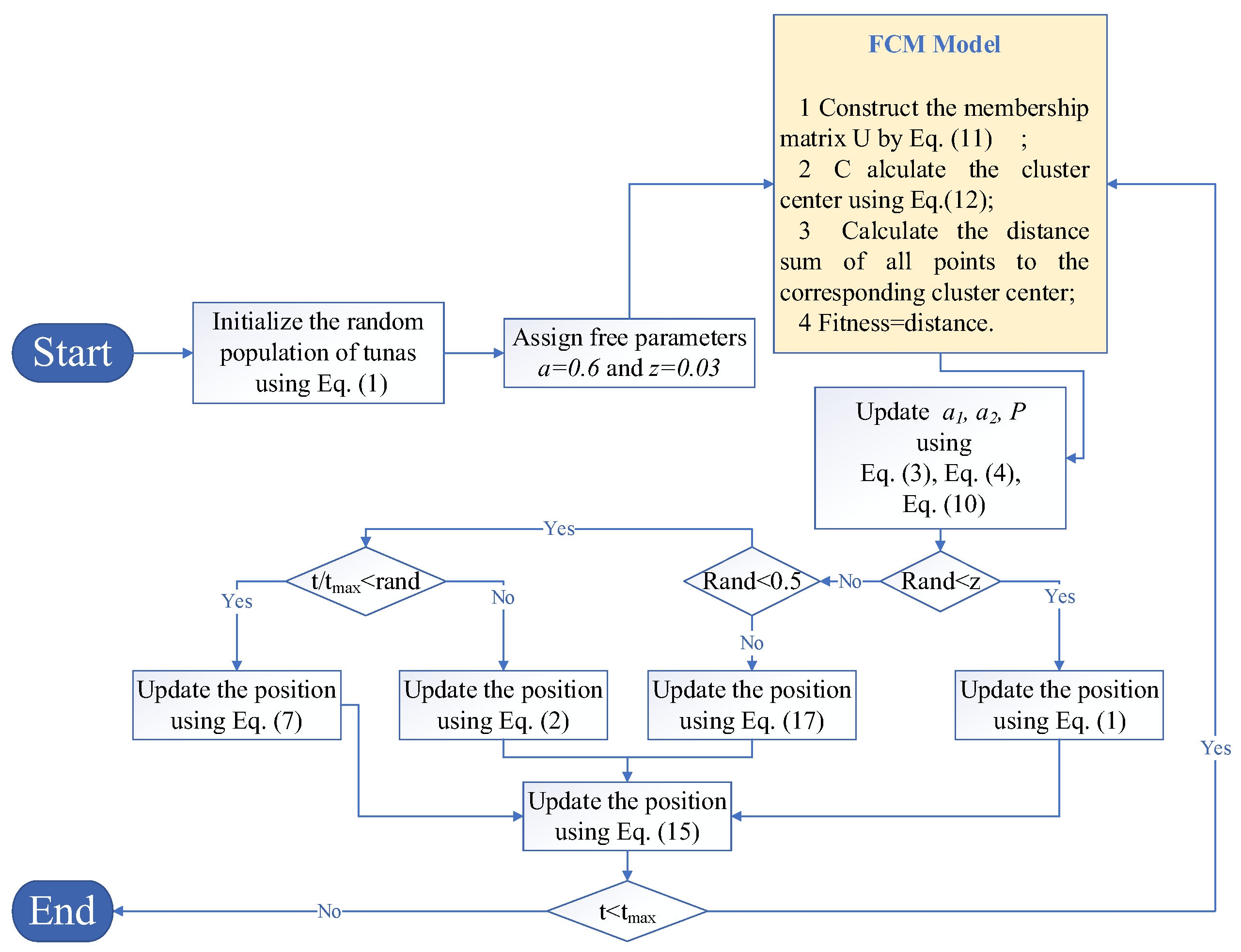
The process of MSTSO optimizing the FCM cluster is as follows: the flowchart is shown in Figure 1; the pseudo-code is shown in Algorithm 2.

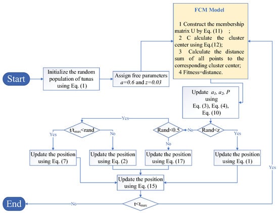
Figure 1. MSTSO optimizes the FCM cluster.

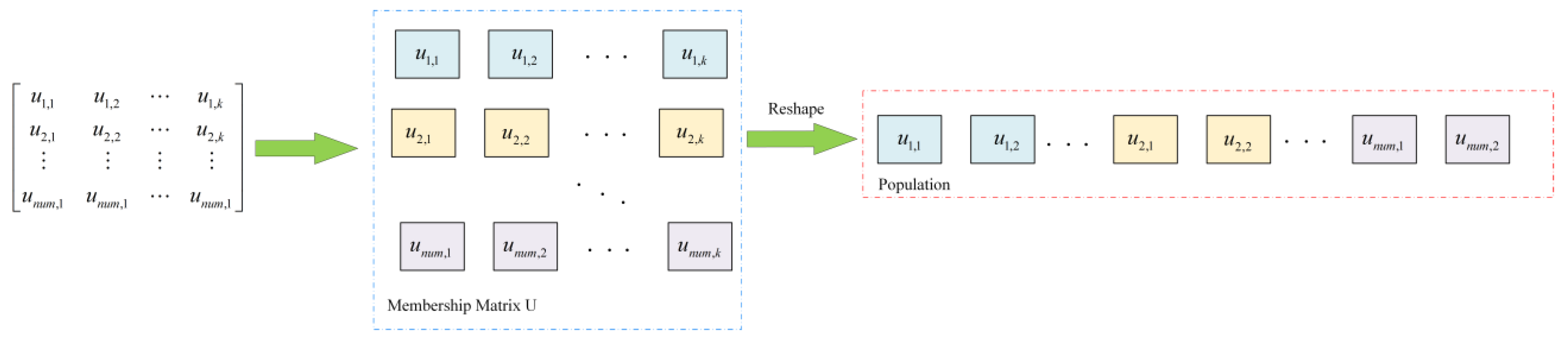
Step 1: Use Equation (1) to randomly initialize the population and assign the parameters a and z, where $\dim =k\cdot num$ means the population dimension, with each dimension including all the elements in the membership matrix $U$, as shown in Figure 2:

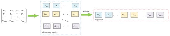
Figure 2. Membership matrix U reshaped to the population in MSTSO.

Step 2: Introduce the FCM module to calculate the fitness value. Equation (11) is used to reconstruct the membership matrix into the data, in which the dimension of each population and the number of parameters of the membership matrix in the MSTSO algorithm are the same and Equation (12) is used to calculate the cluster center point, and finally the sum of the distances from all arrays to the cluster center is calculated, as shown in the following:

$$distance={\displaystyle \sum _{l=1}^k\Vert x_i-c_l\Vert }$$

(22)

Step 3: Update the population position and calculate the fitness value. Update $a_1,a_2,p$. When random number $rand<z$, use Equation (1) to initially update the population position. When $rand>z$, make a finer division. Use Equation (13) to initially update the position, and vice versa. When $t/t_{\max }<rand$, use Equation (7) to conduct a preliminary update. When $t/t_{\max }>rand$, use Equation (2) to perform a preliminary update and finally use Equation (11) to again update the position information that enters the FCM model before calculating the fitness value.

Step 4: Determine whether the iteration is terminated. When the iteration is terminated, output the membership matrix U corresponding to the optimal fitness value at this time. As the optimal FCM model is constructed, if the iteration termination condition is not met, return to Step 2.

Algorithm 2: The procedure of MSTSO-FCM
Input:	fFCM, [Xmin, Xmax], FEsmax.
Output:	membership matrix U
1.	Reshape the membership matrix U to population X using Equation (11);
2.	Initialize population X by using Equation (1);
3.	Assign a = 0.6 and z = 0.03
5.	Evaluate X to determine their fitness value by using fFCM(X) (Equation (22)).
6.	Update Fes using Fes = Fes + NPFes = Fes + NP
7.	Execute MSTSO’s Main Loop;
8.	Reshape the xbest. to U, and output.

4. Simulation Experiment and Comparative Analysis

4.1. MSTSO Algorithm Performance Verification

To illustrate the performance of the MSTSO algorithm proposed in this paper, the CEC2017 test set is selected for verification, including 1 unimodal function, 7 multimodal functions, 10 mixed functions, and 10 combined functions. All simulations in this paper are run on MATLAB R2016b software, and the experimental environment is an Intel(R) Core^(TM) i7-8700 CPU, 16 GB memory computer. In this paper, the butterfly optimization algorithm (BOA), reptile search algorithm (RSA), arithmetic optimization algorithm (AOA), tunicate swarm algorithm (TSA), and sparrow search algorithm (SSA) are selected as comparison algorithms to illustrate the performance of the improved algorithm MSTSO. To ensure the fairness of the experiment, the population of all algorithms is 500, the maximum number of iterations is 600, and the parameter settings of the rest of the algorithms are based on the parameter values of the original paper. Each algorithm runs independently 51 times, and the statistical average results are shown in Appendix A.

From Appendix A, we can see that MSTSO performs well on most test functions. Specifically, for the unimodal test function F1, although MSTSO fails to stably obtain the optimal solution, the MSTSO optimization accuracy is significantly better than that of other algorithms, reaching nine orders of magnitude, illustrating that MSTSO has excellent local search ability. The multimodal functions F2–F8 are often used to test the global search ability of algorithms, which usually have multiple local minimums, so excellent algorithms can jump out of local minima to obtain global optimal values. MSTSO performs best on all seven of these functions, ranking behind RSA only on F8. For TSO, MSTSO performs better on all multimodal functions, indicating that MSTSO’s improvement strategy significantly improves TSO’s global search ability. F9–F18 and F19–F28 are mixed and combination functions, respectively. These two types of functions have complex structures better able to test the ability of algorithms to solve complex optimization problems. As can be seen from Appendix A, MSTSO ranked second only on F19. In the remaining mixed functions and combination functions, MSTSO is the best performer, achieving significantly better results than TSO, which shows that the improvement strategy proposed in this paper has well enhanced the ability of algorithms to solve complex structural problems. It has the potential to better solve complex optimization problems in the real world.

Appendix B illustrates the p-values calculated by the Wilcoxon signed rank test for each function of each algorithm. If the value is less than 0.05, it means that there is a significant difference between MSTSO and the other competitors; otherwise, there is no significant difference. It can be seen that MSTSO is significantly different from the other algorithms for most functions except for F20. In summary, MSTSO can strike a balance between the development and exploration capabilities of the algorithm and has a good local optimal avoidance ability, which can effectively avoid the premature convergence of the algorithm.

4.2. Cluster Dataset and Comparison Algorithm

To verify the clustering ability of MSTSO-FCM, two sets of artificial large datasets and four sets of UCI datasets are selected [30] and are available from https://archive.ics.uci.edu/datasets (accessed on 3 January 2024), of which two sets of artificial datasets contain three categories, with each category containing 5000 sets of data, respectively, two-dimensional characteristic data and three-dimensional characteristic data, which conformed to Gaussian distribution, and the basic information of the data is shown in Table 1.

Table 1. Information about the dataset.

Dataset Name	Number of Data Objects	Characteristic Dimensions	Categorized Categories
Artificial data set1	15,000	2	3
Artificial data set1	15,000	3	3
UCI-iris	150	4	2
UCI-liver	345	6	2
UCI-heart	303	13	2
UCI-pima	768	8	2
UCI-waveform	5000	21	3

To evaluate the clustering performance of each algorithm, three clustering indicators, Accuracy (Ac), Silhouette (Sil), Davies-Bouldin (DB), and Area Under Curve (AUC) are introduced, and the specific information of each index is shown in Table 2.

Table 2. Cluster indicators.

Indicators	Equations	Specific Information
Ac	$A=\frac{N_r}{N}\times 100$	$N_r$ is the correct sample classification number, $N$ is the total number of samples. The larger the value of A, the better the clustering.
Sil	$SI=\frac{1}{N}{\displaystyle {\sum }_{i=1}^N\frac{b_i-a_i}{\max (b_i,a_i)}}$	$SI\in \left[-1,1\right]$ The larger the value $SI$, the better the clustering effect. $a_i$ denotes the mean of the distance from the sample i to each sample in the set. $b_i$ denotes the mean of the distance from sample i to each sample in the nearest set.
DB	$DB=\frac{1}{k}{\displaystyle {\sum }_{j=1}^k\max (\frac{s(c_j)+s(c_r)}{dist(c_j,c_r)})}$	The ratio of the sum of scatters within a cluster between cluster separations. $s(c_j)$ denotes the mean distance from the center point $c_j$ of the set for all points in the set. $s(c_r)$ denotes the mean distance from the center point $c_r$ of the set for all points in the set.
AUC	$AUC=\frac{{\displaystyle {\sum }_{\mathrm{ins}\in p}ran{k}_{ins}-\frac{M\times (M+1)}{2}}}{M\times N}$	$M,N$ represents the number of positive and negative samples, ${\displaystyle {\sum }_{\mathrm{ins}\in p}}$ represents the adding of the positive sample numbers, $ran{k}_{ins}$ represents the i-th Sample.

Four comparison algorithms are selected, namely the TSO-FCM algorithm, PSO-FCM algorithm [13], FCM algorithm, Gaussian mixed clustering (GMM) [31], and K-means clustering algorithm [32]. Table 3 shows the clustering algorithm parameters.

Table 3. Comparison algorithm settings.

Number	Algorithm	Parameter Settings
1	MSTSO-FCM	The index of membership matrix $M=4$, Maximum iterations $I=100$, Termination condition $E=1\cdot e^{-6}$ $z=0.05,a=0.7$.
2	TSO-FCM	$M=4$, $I=100$, $E=1\cdot e^{-6}$ $z=0.05,a=0.7$.
3	PSO-FCM	$M=4$, $I=100$, $E=1\cdot e^{-6}$, $C_1=C_2=1.4$.
4	FCM	$M=4$, $I=100$, $E=1\cdot e^{-6}$.
5	GMM	Non-negative regularized number $n_n=1\cdot e^{-5}$.
6	K-MEANS	The number of clusters varies with the dataset.

4.3. Evaluation of Clustering Results

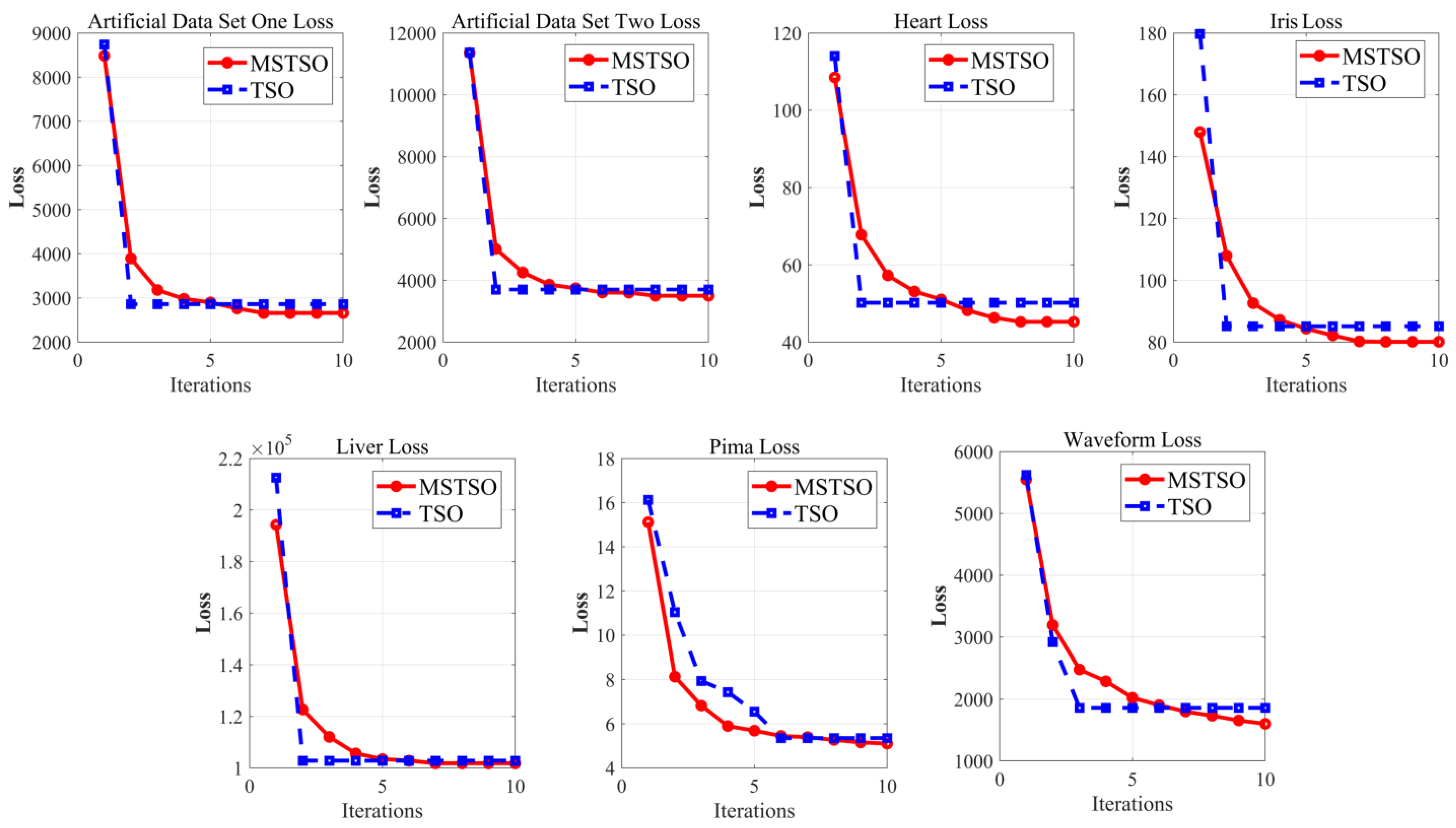
To verify that MSTSO can achieve a better improvement effect on FCM clustering, in the above five datasets, the loss reduction curve of the traditional TSO algorithm is compared. The loss reduction curve is a curve in which the value of the loss function changes as the number of times it is learned increases. The comparison results are shown in Figure 3, in which the convergence ability of MSTSO in the early stage is not as good as that of TSO, but its development performance is better. After TSO stagnates, MSTSO can still search for a better development posture. Generally, after iterating to 8 times, MSTSO will stagnate. From the decline curve of the UCI public data set in the figure, it can be intuitively seen that the late convergence ability of MSTSO is stronger than that of traditional TSO, and it can better explore the global situation and obtain smaller loss values.

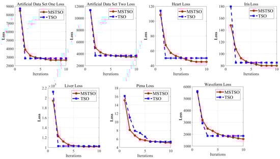
Figure 3. MSTSO optimization and TSO optimization loss reduction curve comparison.

To further verify the clustering effect, AC, Sil, DB, and AUC are used for evaluation, in which AC indicates the clustering accuracy, Sil and DB represent the internal indicators of the cluster, and AUC is to evaluate the classification ability of positive and negative cases of the cluster. It can be seen from Table 4 that MSTSO-FCM has achieved the best score in the AC indicators of the six datasets. In addition, there is significant progress compared with TSO-FCM, PSO-FCM, and FCM. It has good clustering ability. MSTSO-FCM also has progressed in the Sil index. For artificial dataset 1, the Sil index of FCM is only 0.60, the Sil index of TSO-FCM is 0.74 compared with FCM, and the Sil value of PSO-FCM is 0.73. However, the Sil index of MSTSO-FCM reaches 0.84, showing that the discrimination between clusters is significantly improved on dataset 1. On dataset 2, the DB index of FCM is 1.39, while the DB index of TSO-FCM on dataset 2 is 0.87, the DB index of PSO-FCM is 0.85, and the DB index of MSTSO-FCM on dataset 2 is 0.4735. Compared with TSO-FCM and PSO-FCM, the intra-cluster compactness and inter-cluster separation have been improved, and the clustering effect is better. Regarding the AUC index, MSTSO-FCM achieved first in the four groups of UCI data sets, and had significant advantages compared with TSO-FCM and PSO-FCM, indicating that MSTSO-FCM has excellent classification ability.

Table 4. Comparison of clustering performance results.

Algorithm	Dating	AC	Sil	DB	AUC	Algorithm	Dating	AC	Sil	DB	AUC
MSTSO-FCM	set1	97.13%	0.84	0.15	0.96	FCM	set1	89.97%	0.60	0.45	0.88
	set2	90.04%	0.61	0.47	0.90		data	75.19%	0.26	1.39	0.74
	iris	98.67%	0.50	0.64	0.97		iris	90.67%	0.54	0.59	0.89
	liver	63.48%	0.23	2.48	0.62		liver	50.14%	0.51	1.17	0.51
	heart	89.44%	0.13	2.49	0.90		heart	74.59%	0.19	1.93	0.72
	pima	69.12%	0.19	2.34	0.65		pima	58.18%	0.32	2.72	0.55
	waveform	77.62%	0.58	0.75	0.75		waveform	65.84%	0.51	0.89	0.64
PSO-FCM	set1	92.7%	0.73	0.26	0.91	GMM	set1	89.71%	0.12	0.77	0.86
	set2	77.45%	0.39	0.85	0.75		set2	73.26%	0.21	1.46	0.72
	iris	92.67%	0.46	0.59	0.91		iris	96.67%	0.50	0.65	0.95
	liver	57.97%	0.34	1.90	0.55		liver	50.14%	0.50	1.07	0.51
	heart	79.54%	0.21	2.39	0.77		heart	54.78%	0.18	2.12	0.53
	pima	65.17%	0.25	2.19	0.62		pima	61.93%	0.11	2.20	0.62
	waveform	70.37%	0.52	0.82	0.69		waveform	70.62%	0.53	1.21	0.68
TSO-FCM	set1	94.8%	0.74	0.25	0.93	K-Means	set1	80.54%	0.36	0.97	0.80
	data	79.36%	0.38	0.87	0.77		set2	70.12%	0.18	1.59	0.68
	iris	94.67%	0.51	0.64	0.93		iris	89.33%	0.55	0.58	0.88
	liver	56.81%	0.33	1.92	0.59		liver	46.00%	0.63	0.77	0.48
	heart	80.86%	0.15	2.25	0.78		heart	72.61%	0.21	1.82	0.71
	pima	66.26%	0.23	2.51	0.63		pima	66.92%	0.17	1.78	0.67
	waveform	72.42%	0.56	0.79	0.61		waveform	60.12%	0.35	1.98	0.89

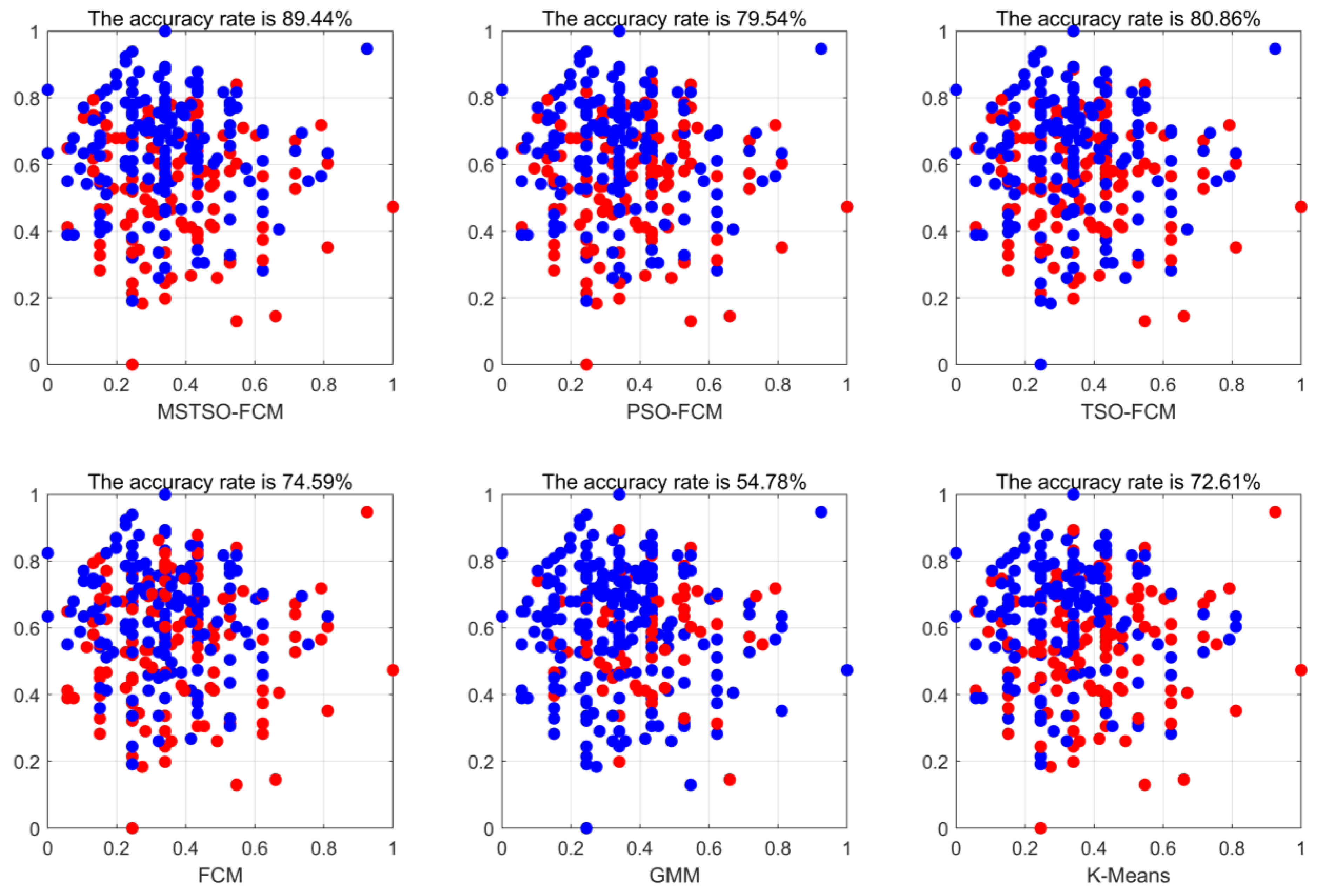
To visualize the clustering effect, the two-dimensional features of the dataset Heart are selected for display. Each color in Figure 4 corresponds to a cluster, and the same color representation of different algorithms may not be the same, but it does not affect the results. It can be seen from the figure that MSTSO-FCM has achieved better clustering results than FCM, TSO-FCM, and PSO-FCM.

Figure 4. Heart dataset two-dimensional feature clustering effect visualization.

It can be seen from Table 4 that MTSO-FCM can achieve better classification results in a variety of different sample situations. Compared with FCM, MTSO-FCM overcomes the data sensitivity better and shows excellent classification performance. It can be seen from the AUC index that this algorithm has a better classification ability of positive and negative cases. In Figure 3, the MSTSO algorithm has a better global search ability. However, its computational complexity has not been significantly improved, and it is an improvement on the traditional hard clustering algorithm.

5. Conclusions

In this paper, a clustering algorithm of MSTSO-FCM is proposed, which first integrates the chaotic local search strategy and the shift distribution estimation strategy into the TSO algorithm, which improves the performance of basic TSO by enhancing the development ability and maintaining population diversity. Secondly, the search and development characteristics of the MSTSO algorithm are introduced into the fuzzy matrix of FCM, which overcomes the defects of poor global search ability and sensitive initialization. It not only uses the searchability of MSTSO but also retains the fuzzy mathematical ideas of FCM, to improve the clustering accuracy, stability, and accuracy of the FCM algorithm. In two groups of artificial datasets and four groups of UCI datasets, MSTSO-FCM achieves the first good results in the AC index and AUC index, indicating that it has excellent clustering and classification ability, and has significant improvement compared with TSO-FCM and PSO-FCM in Sil and DB two internal indicators; this shows that the intra-cluster compactness and inter-cluster separation have been improved. The simulation results show that the improved clustering algorithm has better convergence ability and clustering effect.

In the future research direction, the density clustering method will be studied, FCM will be combined with density clustering, and it is necessary to focus more on solving real-world engineering application problems.

References

- Atluri, G.; Karpatne, A.; Kumar, V. Spatio-temporal data mining: A survey of problems and methods. Acm Comput. Surv. 2018, 51, 1–41. [Google Scholar] [CrossRef]
- Jia, H.M.; Jiang, Z.C.; Li, Y. Simultaneous feature selection optimization based on improved bald eagle search algorithm. Control Decis. 2022, 37, 445–454. [Google Scholar]
- Banerjee, D. Recent progress on cluster and meron algorithms for strongly correlated systems. Indian J. Phys. 2021, 95, 1669–1680. [Google Scholar] [CrossRef]
- Mohapatra, S.K.; Sahu, P.; Almotiri, J.; Alroobaea, R.; Rubaiee, S.; Bin Mahfouz, A.; Senthilkumar, A.P. Segmentation and classification of encephalon tumor by applying improved fast and robust FCM Algorithm with PSO-based ELM Technique. Comput. Intell. Neurosci. 2022, 2002, 1–9. [Google Scholar] [CrossRef]
- Mehran, M.; Ali, K.; Hamed, H. Clustering-based reliability assessment of smart grids by fuzzy c-means algorithm considering direct cyber–physical interdependencies and system uncertainties. Sustain. Energy Grids Netw. 2002, 31, 100757. [Google Scholar]
- Yang, Q. An FCM clustering algorithm based on the identification of accounting statement whitewashing behavior in universities. J. Intell. Syst. 2022, 31, 345–355. [Google Scholar] [CrossRef]
- Poli, R.; Kennedy, J.; Blackwell, T. Particle swarm optimization. Swarm Intell. 2007, 1, 33–57. [Google Scholar] [CrossRef]
- Maryam, M.; Reza, S.A.; Arash, D. Optimization of fuzzy c-means (FCM) clustering in cytology image segmentation using the gray wolf algorithm. BMC Mol. Cell Biol. 2022, 23, 9. [Google Scholar]
- Amit, B.; Issam, A. A novel adaptive FCM with cooperative multi-population differential evolution optimization. Algorithms 2022, 15, 380. [Google Scholar]
- Niknam, T.; Olamaei, J.; Amiri, B. A Hybrid Evolutionary Algorithm Based on ACO and SA for Cluster Analysis. J. Appl. Sci. 2008, 8, 2695–2702. [Google Scholar] [CrossRef]
- Gao, H.; Li, Y.; Kabalyants, P.; Xu, H.; Martinez-Bejar, R. A Novel Hybrid PSO-K-Means Clustering Algorithm Using Gaussian Estimation of Distribution Method and Lévy Flight. IEEE Access 2020, 8, 122848–122863. [Google Scholar] [CrossRef]
- Izakian, H.; Abraham, A. Fuzzy C-means and fuzzy swarm for fuzzy clustering problem. Expert Syst. Appl. 2011, 38, 1835–1838. [Google Scholar] [CrossRef]
- Qian, Z.; Cao, Y.; Sun, X.; Ni, L.; Wang, Z.; Chen, X. Clustering optimization for triple-frequency combined obser-vations of BDS-3 based on improved PSO-FCM algorithm. Remote Sens. 2022, 14, 3713. [Google Scholar] [CrossRef]
- Celal, O.; Emrah, H.; Dervis, K. Dynamic clustering with improved binary artificial bee colony algorithm. Appl. Soft Comput. 2015, 28, 69–80. [Google Scholar]
- Wang, J.; Zhu, L.; Wu, B.; Ryspayev, A. Forestry Canopy Image Segmentation Based on Improved Tuna Swarm Optimization. Forests 2022, 13, 1746. [Google Scholar] [CrossRef]
- Wang, W.; Tian, J. An Improved Nonlinear Tuna Swarm Optimization Algorithm Based on Circle Chaos Map and Levy Flight Operator. Electronics 2022, 11, 3678. [Google Scholar] [CrossRef]
- Tuerxun, W.; Xu, C.; Guo, H.; Guo, L.; Zeng, N.; Cheng, Z. An ultra-short-term wind speed prediction model using LSTM based on modified tuna swarm optimization and successive variational mode decomposition. Energy Sci. Eng. 2022, 10, 3001–3022. [Google Scholar] [CrossRef]
- Tan, M.; Li, Y.; Ding, D.; Zhou, R.; Huang, C. An Improved JADE Hybridizing with Tuna Swarm Optimization for Numerical Optimization Problems. Math. Probl. Eng. 2022, 2022, 1–17. [Google Scholar] [CrossRef]
- Awad, A.; Kamel, S.; Hassan, M.H.; Elnaggar, M.F. An Enhanced Tuna Swarm Algorithm for Optimizing FACTS and Wind Turbine Allocation in Power Systems. Electr. Power Compon. Syst. 2023. [Google Scholar] [CrossRef]
- Kumar, C.; Mary, D.M. A novel chaotic-driven Tuna Swarm Optimizer with Newton-Raphson method for parameter identification of three-diode equivalent circuit model of solar photovoltaic cells/modules. Optik 2022, 264, 169379. [Google Scholar] [CrossRef]
- Ren, Q.; Zhang, H.; Zhang, D.; Zhao, X. Lithology identification using principal component analysis and particle swarm optimization fuzzy decision tree. J. Pet. Sci. Eng. 2023, 220, 111233. [Google Scholar] [CrossRef]
- Wu, T.-Y.; Lin, J.C.-W.; Zhang, Y.; Chen, C.-H. A Grid-Based Swarm Intelligence Algorithm for Privacy-Preserving Data Mining. Appl. Sci. 2019, 9, 774. [Google Scholar] [CrossRef]
- Shao, Y.; Lin, J.C.-W.; Srivastava, G.; Guo, D.; Zhang, H.; Yi, H.; Jolfaei, A. Multi-Objective Neural Evolutionary Algorithm for Combinatorial Optimization Problems. IEEE Trans. Neural Netw. Learn. Syst. 2021, 34, 2133–2143. [Google Scholar] [CrossRef]
- Kubicek, J.; Varysova, A.; Cerny, M.; Skandera, J.; Oczka, D.; Augustynek, M.; Penhaker, M. Novel Hybrid Optimized Clustering Schemes with Genetic Algorithm and PSO for Segmentation and Classification of Articular Cartilage Loss from MR Images. Mathematics 2023, 11, 1027. [Google Scholar] [CrossRef]
- Aggarwal, A.; Dimri, P.; Agarwal, A.; Verma, M.; Alhumyani, H.A.; Masud, M. IFFO: An Improved Fruit Fly Optimization Algorithm for Multiple Workflow Scheduling Minimizing Cost and Makespan in Cloud Computing Environments. Math. Probl. Eng. 2021, 2021, 1–9. [Google Scholar] [CrossRef]
- Aggarwal, A.; Kumar, S.; Bhatt, A.; Shah, M.A. Solving User Priority in Cloud Computing Using Enhanced Optimization Algorithm in Workflow Scheduling. Comput. Intell. Neurosci. 2022, 2022, 1–11. [Google Scholar] [CrossRef] [PubMed]
- Upadhyay, P.; Marriboina, V.; Kumar, S.; Kumar, S.; Shah, M.A. An Enhanced Hybrid Glowworm Swarm Optimization Algorithm for Traffic-Aware Vehicular Networks. IEEE Access 2022, 10, 110136–110148. [Google Scholar] [CrossRef]
- Balaji, P.; Muniasamy, V.; Bilfaqih, S.M. Chimp Optimization Algorithm Influenced Type-2 Intuitionistic Fuzzy C-Means Clustering-Based Breast Cancer Detection System. Cancers 2023, 15, 1131. [Google Scholar] [CrossRef] [PubMed]
- Usman, Q. A dissimilarity measure based fuzzy c-means (FCM) clustering algorithm. J. Intell. Fuzzy 2014, 26, 229–238. [Google Scholar]
- Tanveer, M.; Gautam, C.; Suganthan, P. Comprehensive evaluation of twin SVM based classifiers on UCI datasets. Appl. Soft Comput. 2019, 83, 105617. [Google Scholar] [CrossRef]
- Ma, Y.; Hao, Y. Antenna Classification Using Gaussian Mixture Models (GMM) and Machine Learning. IEEE Open J. Antennas Propag. 2020, 1, 320–328. [Google Scholar] [CrossRef]
- Mao, B.; Li, B. Building façade semantic segmentation based on K-means classification and graph analysis. Arab. J. Geosci. 2019, 12, 1–9. [Google Scholar] [CrossRef]
Disclaimer/Publisher’s Note: The statements, opinions and data contained in all publications are solely those of the individual author(s) and contributor(s) and not of MDPI and/or the editor(s). MDPI and/or the editor(s) disclaim responsibility for any injury to people or property resulting from any ideas, methods, instructions or products referred to in the content. |
© 2024 by the authors. Licensee MDPI, Basel, Switzerland. This article is an open access article distributed under the terms and conditions of the Creative Commons Attribution (CC BY) license (https://creativecommons.org/licenses/by/4.0/).