Abstract
In this work, the susceptible-infectious-removed (SIR) dynamics are considered in relation to the effects on the health system. With the help of the Caputo derivative fractional-order method, the SIR epidemic model for childhood diseases is designed. Subsequenly, a set of sufficient conditions ensuring the existence and uniqueness of the addressed model by choosing proper fuzzy approximation methods. In particular, the fuzzy Laplace method along with the Adomian decomposition transform were employed to better understand the dynamical structures of childhood diseases. This leads to the development of an efficient methodology for solving fuzzy fractional differential equations using Laplace transforms and their inverses, specifically with the Caputo sense derivative. This innovative approach facilitates the numerical resolution of the problem and numerical simulations are executed for considering parameter values.
Keywords:
susceptible-infectious-removed dynamics; fractional-order model; fuzzy systems; Caputo derivative; existence and uniqueness MSC:
03C45; 34D20; 34A07; 34A08; 39A30
1. Introduction
One of the most well-known fields of study in the biological sciences that looks into how disease, health, and other related factors are designed at the population level is called epidemiology. The term epidemiology is derived from the greek word ‘epi’, meaning upon, ‘demo’, meaning people, and ‘logos’, meaning study. This etymology indicates that only human populations are included in discussions of epidemiology (see [1]). One of the rich areas of applications and research for mathematics in biological sciences today is the widely studied field of infectious illnesses. Evidently, contagious diseases significantly increase both the morbidity and mortality rates of both the human race and our target populations of non-human animals.
The most severe infectious infections are those that affect children. Famous among these are rubella, poliomyelitis, and measles. A respiratory infection by a Morbillivirus causes the highly contagious disease known as measles. Children are typically affected by these diseases because they are more likely to spread among them than among adults. Thus, two broad categories, namely the premature populations and mature populations, can be made to describe the population. Maturation delay occurs when the infant population takes a consistent amount of time to mature. A disease-latent phase is determined by the dynamics of the disease in question, which means the amount of time required for the disease to become fully active in the body. Immunization is an essential approach to the global management of pediatric illnesses.
Since children’s immune systems are so fragile, they are all exposed to a wide range of infectious and noninfectious disorders while they are still young. The most prevalent pediatric illnesses are either bacterial or viral infections, as well as allergy and immunologic conditions. Children who contract the “rotavirus” infection experience diarrhea, high fever, and vomiting, which frequently worsens dehydration issues. The “chickenpox” virus is called “varicella”. Measles, commonly known as “German measles”, is brought on by the “rubeola virus”, which can have fatal consequences. Many juvenile diseases cannot spread quickly through the body of a human being; instead, they require a period called the “latent period” to manifest. To prevent all of the aforementioned pediatric illnesses, appropriate vaccination is advised on a global scale. In 1974, the WHO began a global immunization program with this goal in mind. A mathematical model can help understand how a disease spreads and offers various methods for controlling its spread. Numerous writers, scientists, and biologists, including Haq et al. [2], Ahmed et al. [3], and Kumar [4], have used a variety of analytical and numerical techniques to solve different types of bio-mathematical epidemic models. Many scientists have demonstrated over the last few decades that fractional models can more precisely explain natural occurrences than integer order differential equations. Because of this benefit, the fractional calculus has gained prominence in modeling realistic problems, particularly those with memory effects [5,6]. Furthermore, fractional calculus and mathematical modeling are used in various domains such as social sciences, engineering, and mathematical biology [7]. In 2017, the SIR model was used to discuss a fractional model of infection and recovery [8]. In [9], the SIR epidemic system, which explains a non-linear recurrence % with arbitrary order, was investigated. In [10], the authors discuss arbitrary-order SIR epidemic system solutions. In the same year, Srivastava et al. discussed the SIR epidemic system of children diseases in their article [11]. There are currently several studies active to examine the COVID-19 virus models in various ways (see [12]).
The future transmission of the disease will be caused by past events and their cumulative impact on earlier volumes. The inheritance trait and history effect reveal the spread of already infected patients. Therefore, the effects of these features on the transmission of a disease can be studied using fractional derivatives. The latest additions to present calculus and differential equations (DE) are fuzzy calculus and fractional order differential equations (FODE), respectively. In recent years, FO modeling has developed into a fruitful and stimulating area of study from a variety of angles. It is possible to illustrate arbitrary-order derivatives and integrals with singular and non-singular kernels in a variety of ways. The definition of many types of fractional derivatives, which in turn led to intriguing theories of fractional calculus, was greatly aided by the Mittag–Leffler (ML) function. Indeed, because of the frequent use of ML in engineering and real-world issues during the past five years, scientists and engineers’ vital interests in the field have significantly expanded (see [13,14]). To support the existence and uniqueness theory of solutions, several academics have studied FODEs and fuzzy integral equations [15,16,17]. It takes a long time to come up with more precise solutions for each fuzzy FODE when using them. Mathematicians have examined fuzzy FODEs in depth using a wide range of techniques, including perturbation methods, integral transform methods, and spectral techniques. Uncertainty, which expresses the unpredictability and computational difficulty of a system, is an essential concept in mathematical modeling.
According to the above facts, we consider a fuzzy fractional-order childhood disease model under the Caputo derivative. The main contributions of this paper are as follows:
- As a first attempt, in this paper, a fuzzy fractional Caputo derivatives approach subject to a SIR dynamic is developed for childhood dieases.
- The fixed point theorem of Schauder and Banach is used to demonstrate the existence and uniqueness of the solution to the addressed model.
- Perform the numerical simulations by using fuzzy Laplace and inverse Laplace transform based on the Adomian decomposition method.
- Numerical results shows the validity and effectiveness of the tracking performance of the proposed fuzzy fractional SIR dynamic.
The structure of the article is as follows. The fundamental idea of fuzzy and fuzzy fractional Caputo derivative is described in Section 2. In Section 3, the fuzzy fractional Caputo derivative model formulation has been briefly explained. The existence and uniqueness of the thallae solution of the model is established in Section 4. The scheme of the solution is described in Section 5. The numerical approximations are also provided in Section 6 for theoretical support and, finally, the conclusion is given in Section 7.
2. Preliminaries
Firstly, the following definitions will be required for the convenience of analysis.
Definition 1
([18]). Let be an ambiguous collection of the real line meeting the requirements as follows: ν should be normal (for any ), the upper semicontinuous on , should be convex, and should be compact.
Definition 2
([19]). For the fuzzy number ν, the definition of the β-level set is given by
where and .
Definition 3
([20]). The following describes the fuzzy number’s parametric form: , where , meeting the requirements below:
- should be bounded, increasing function, right continuous at 0 and left continuous over .
- should be bounded, decreasing over , right continuous at 0.
- should be less than or equal to .
Also, if , then ω is called a crisp number.
Definition 4
([20]). is taken to be a mapping. Let and be the two fuzzily represented integers in parametric form. The Hausdorff distance, which is a measure of the separation between p and q, is defined as
In E, the metric α shall have the following properties:
- 1.
- for all ;
- 2.
- for all ;
- 3.
- for all ;
- 4.
- is a complete metric space.
Definition 5
([19]). Let . If there exist such that then is said to be the H-difference of and , represented by .
Definition 6
([21]). Let be a fuzzy mapping. Then, Θ is called continuous if for any and a fixed value of , we have
Definition 7
([22]). By allowing ω to be a continuous fuzzy function on , we may define a fuzzy fractional integral in the Riemann–Liouville sense that corresponds to t.
Consider , where and are the spaces of fuzzy continuous functions and fuzzy Lebesgue integrable functions, respectively. The fuzzy fractional integral is defined as follows.
where
Definition 8
([16]). If a fuzzy function is such that , and , then the fuzzy fractional Caputo’s derivative is defined as
where
whenever and the integrals on the right sides converge.
3. Formulation of Fuzzy Fractional SIR Model
Fuzzy calculus and fractional order differential equations (FODEs) have lately been added to the realm of differential equations and modern calculus. Then, the definition of FODEs was enlarged to cover fuzzy FODEs [20,21,23]. To prove the existence and uniqueness theory of solutions, many researchers have researched FODEs and fuzzy integral equations, for example, [17,24,25,26,27,28]. When working with fuzzy FODEs, it takes a long time to compute more accurate solutions to each fuzzy FODEs. Numerous methods have been developed by mathematicians to solve fuzzy FODEs, including perturbation methods, integral transform methods, and spectral techniques [5,18,19,22,29,30]. Figure 1 shows the flow chart of the SIR model.
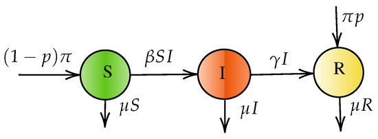
Figure 1.
Flow chart for susceptible-infectious-removed model.
In this study, pay close attention to the following Caputo fractional-order model in [2] with the susceptible population , the infected population , and the removed population being the three groups that make up the entire population and fractional-order :
where the initial states are defined as and .
4. Existence and Uniqueness Results
This section describes the existence and distinctiveness of the solution to the following fuzzy fractional model. The description of the prescribed model is given in Table 1. Here, we looked into a set of fuzzy fractional-order differential equations in the sense of Caputo, which depicts an epidemic model of childhood sickness with initial data uncertainty. For
Now, the right hand side of (2) becomes
where the fuzzy functions are . Then, for model (2) gets the form
with fuzzy initial conditions
Now, using fuzzy fractional integral and using initial conditions, one can get
Banach Space is defined as follows based on the fuzzy norm =.

Table 1.
The description of the prescribed model.
Thus, the Equation (5) is rewritten as
where
In order to obtain the required results, we consider the following assumptions
- There exists a constant and
- There exists constant such that for each we have
Theorem 1.
By using the assumption the prescribed system has atleast one solution.
Proof.
be a convex and closed fuzzy set is considered. Taking the mapping such that
For any , one can obtain
Here, and hence we conclude that is bounded.
Next, completely continuous property of the operator is proved.
For any such that gives
which implies that as As a result, the operator is equi-continuous. The completely continuous nature of the operator is shown by the Arzela–Ascoli theorem. According to Schauder’s fixed point theorem, there is at least one solution to the aforementioned fuzzy fractional model. □
Theorem 2.
The considered system (2) has a single solution under the assumption provided that
Proof.
Let then,
Hence, is a contraction. The Banach contraction principle guarantees that the suggested model (2) has just one solution. □
5. Method Description
The primary goal of this section is to use the Laplace transform (LT) [19,22] to determine how to solve the fuzzy fractional model under consideration. In order to obtain the fuzzy LT model, we have
Under the zero initial condition, one can obtain
which implies that
Based on the infinite series solution, one can obtain
From (2), the nonlinear term can be rewritten as follows:
Here, represents the Adomian polynomial for nonlinear term. The above equations can be obtain that
Taking inverse LT, we have
The terms in the parametric form are compared and we have
and
In light of the aforementioned ideas, it is easy to get the remaining terms. Thus, the generic series solutions are written as follows:
Remark 1.
By using the fixed point theorem and Banach contraction principle, the prescribed model has one solution. In addition, the numerical findings of the fuzzy Laplace transform based on the Adomian decomposition enable the comprehension of the physical behavior of a childhood disease model.
6. Numerical Simulation Results and Discussions
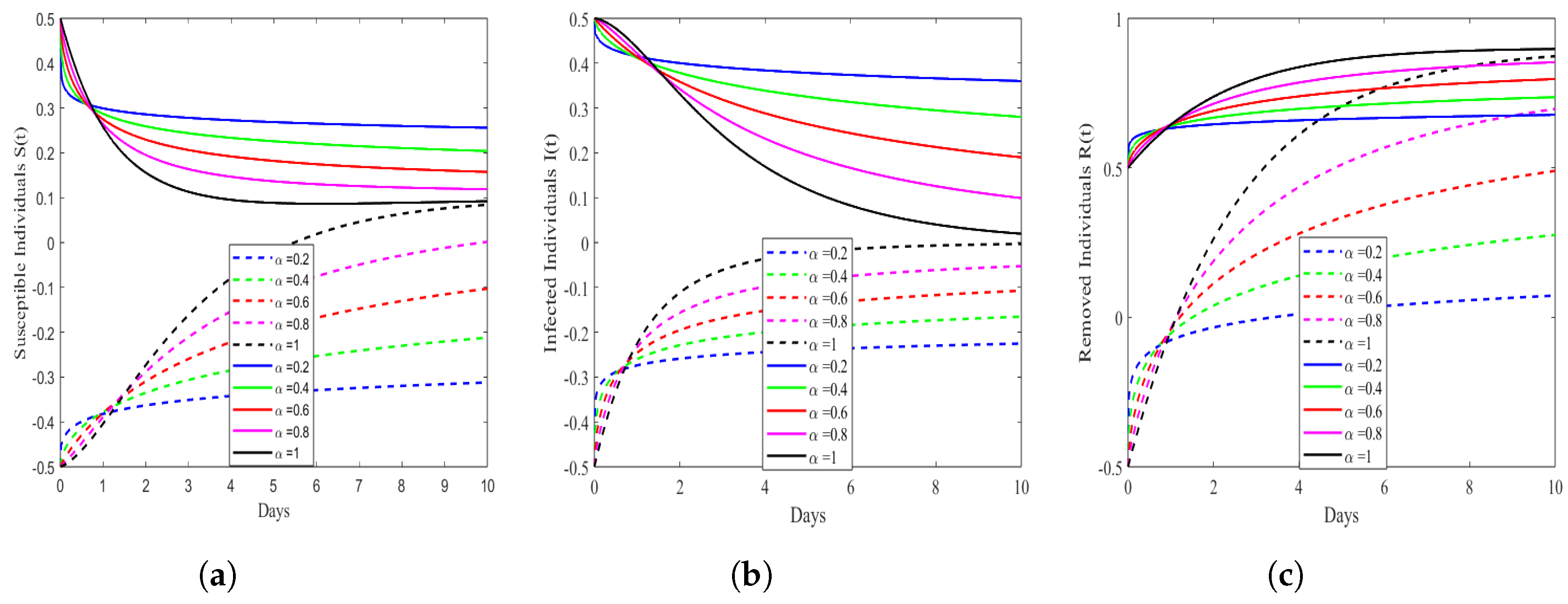
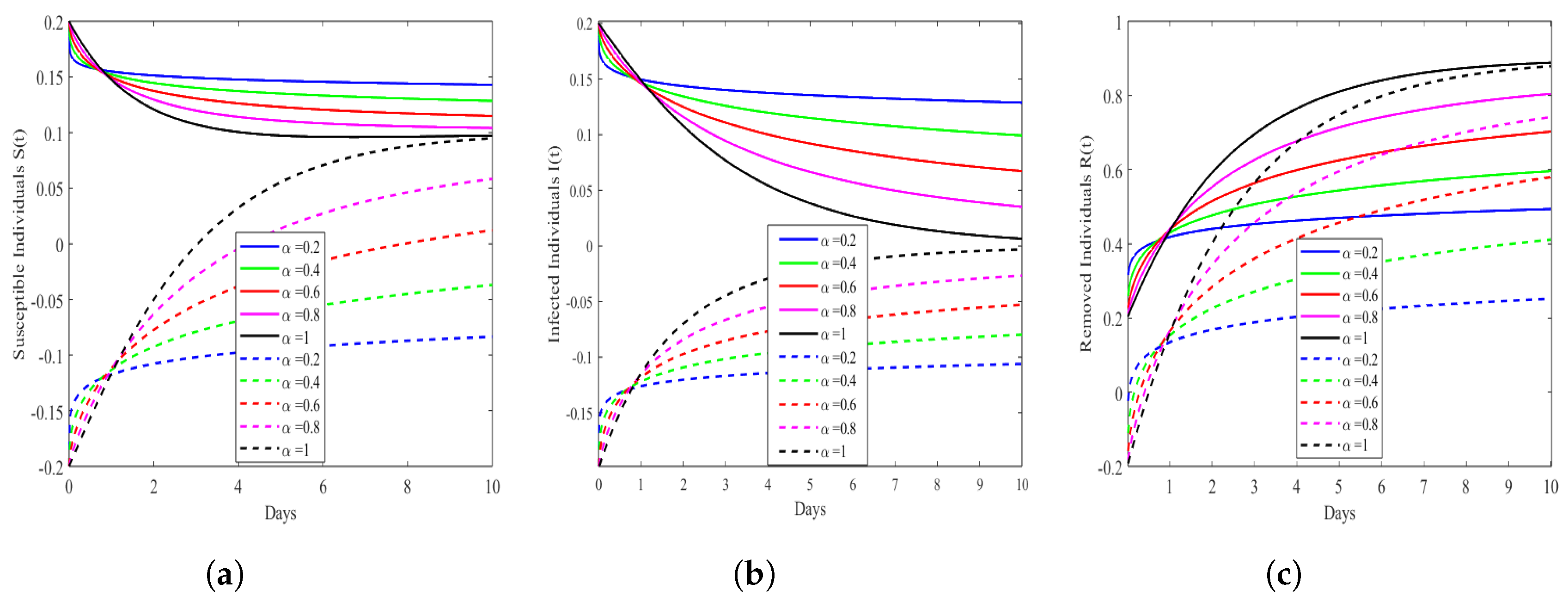
This section provides a numerical example showing the effectiveness of the proposed approach using various parameter values. To find the solution to the FFDEs, a range of numerical and analytical methods can be used. For finding the numerical outcomes, we used MATLAB 2017b. We simulate the numerical results by using different fractional order = 0.2, 0.4, 0.6, 0.8 and 1. The initial conditions are taken as , , and .
From the graphical results it is clear that the result obtained by using the proposed method is very efficient. Furthermore, the present method is also shown to be capable of accurately predicting the behavior of the variables in the region under consideration. As shown in Figure 2 and Figure 3, various compartments exhibit a wide range of dynamics. We effectively utilized various fractional order values, considering uncertainties, to enhance the robustness of our study. By accounting for uncertainties, we strengthened the reliability of our findings, contributing to a more thorough and impactful study. As the susceptible individual value declines, there is a corresponding increase in the infected individual, resulting in the spread of infection at varying rates influenced by distinct fractional orders. From these figures, we can easily observe that the proposed fractional-order method is more efficient in the SIR epidemic model for childhood diseases.
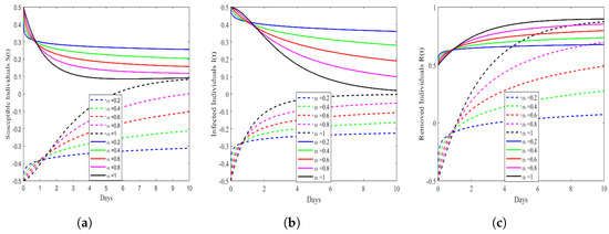
Figure 2.
Simulation result of fuzzy approximations solutions is presented for various fractional order values, with uncertainty set to . Dynamic changes in the transmission of Susceptible (a), Infectious (b), and Removed (c) individuals over days for upper and lower cut representations along with fractional various order.
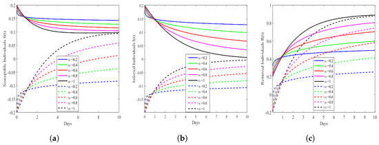
Figure 3.
Simulation result of fuzzy approximate solutions is given in the figure for various values of fractional order is shown, uncertainty . Dynamic changes in the transmission of Susceptible (a), Infectious (b), and Removed (c) individuals over days for upper and lower cut representations along with fractional various order.
7. Conclusions
This research delved into the intricate dynamics of the SIR model, specifically focusing on its implications for the healthcare system. To capture the nuanced behavior of childhood diseases, a novel SIR epidemic model is formulated, leveraging the Caputo derivative fractional-order method. The model’s robustness and singular characteristics are rigorously investigated and confirmed through fixed point theory, establishing the uniqueness and existence of a solution. In order to gain a deeper insight into the dynamic structures inherent in childhood diseases, the study employs two powerful analytical tools: fuzzy Laplace transform and Adomian decomposition transform. By using a fuzzy fractional differential equation with Laplace transformations and their inverses, the numerical results have been obtained for the compartments of the addressed system.
Author Contributions
Conceptualization, S.S., A.K. and S.R.; methodology, S.S., A.K. and S.R.; software, S.S., A.K. and S.R.; validation, S.S., A.K., S.R., P.V., S.D. and K.R.; formal analysis, S.S., A.K. and S.R.; investigation, P.V., S.D. and K.R.; writing—original draft preparation, S.S., A.K. and S.R.; writing—review and editing, S.S., A.K., S.R., P.V., S.D. and K.R.; visualization, S.S., A.K. and S.R.; supervision, P.V., S.D. and K.R. All authors have read and agreed to the published version of the manuscript.
Funding
The work of the sixth author is supported by the Basic Science Research Program through the National Research Foundation of Korea (NRF) funded by the Ministry of Education, South Korea (NRF-2019R1I1A3A02058096 and NRF-2020R1A6A1A12047945), and under the Grand Information Technology Research Center support program IITP-2024-2020-0-01462) supervised by the IITP, South Korea (Institute for Information & Communications Technology Planning & Evaluation).
Data Availability Statement
Data sharing is not applicable to this article as no datasets were generated or analyzed during the current study.
Acknowledgments
The authors are grateful to the anonymous reviewers for their valuable suggestions, which significantly improve the article.
Conflicts of Interest
The authors declare that they have no known competing financial interests or personal relationships that could have appeared to influence the work reported in this paper.
Abbreviations
The following abbreviations are used in this manuscript:
| SIR | Susceptible-Infectious-Removed |
| WHO | World Health Organization |
| DEs | Differential Equations |
| FODEs | Fractional Order Differential Equations |
| ML | Mittag–Leffler |
| LT | Laplace Transform. |
References
- Martcheva, M. An Introduction to Mathematical Epidemiology; Springer: Berlin/Heidelberg, Germany, 2015; Volume 61. [Google Scholar]
- Haq, F.; Shahzad, M.; Muhammad, S.; Wahab, H.A.; ur Rahman, G. Numerical analysis of fractional order epidemic model of childhood diseases. Discret. Dyn. Nat. Soc. 2017, 2017, 1–7. [Google Scholar] [CrossRef]
- Ahmad, A.; Farman, M.; Ahmad, M.; Raza, N.; Abdullah, M. Dynamical behavior of SIR epidemic model with non-integer time fractional derivatives: A mathematical analysis. Int. J. Adv. Appl. Sci 2018, 5, 123–129. [Google Scholar] [CrossRef]
- Kumar, R.; Kumar, S. A new fractional modelling on susceptible-infected-recovered equations with constant vaccination rate. Nonlinear Eng. 2014, 3, 11–19. [Google Scholar] [CrossRef]
- Miller, K.S.; Ross, B. An Introduction to the Fractional Calculus and Fractional Differential Equations, 1st ed.; Springer: Berlin/Heidelberg, Germany, 1993. [Google Scholar]
- Kilbas, A.; Srivastava, H.; Trujillo, J. Theory and Applications of Fractional Differential Equations. In Number v. 13 in North-Holland Mathematics Studies; Elsevier Science: Amsterdam, The Netherlands, 2006. [Google Scholar]
- Baleanu, D.; Diethelm, K.; Scalas, E.; Trujillo, J. Fractional Calculus: Models And Numerical Methods; Series On Complexity, Nonlinearity and Chaos; World Scientific Publishing Company: Singapore, 2012. [Google Scholar]
- Angstmann, C.N.; Henry, B.I.; McGann, A.V. A fractional-order infectivity and recovery SIR model. Fractal Fract. 2017, 1, 11. [Google Scholar] [CrossRef]
- Mouaouine, A.; Boukhouima, A.; Hattaf, K.; Yousfi, N. A fractional order SIR epidemic model with nonlinear incidence rate. Adv. Differ. Equ. 2018, 2018, 1–9. [Google Scholar] [CrossRef]
- Hasan, S.; Al-Zoubi, A.; Freihet, A.; Al-Smadi, M.; Momani, S. Solution of fractional SIR epidemic model using residual power series method. Appl. Math. Inf. Sci. 2019, 13, 153–161. [Google Scholar] [CrossRef]
- Srivastava, H.; Günerhan, H. Analytical and approximate solutions of fractional-order susceptible-infected-recovered epidemic model of childhood disease. Math. Methods Appl. Sci. 2019, 42, 935–941. [Google Scholar] [CrossRef]
- Suganya, S.; Parthiban, V. A mathematical review on Caputo fractional derivative models for COVID-19. AIP Conf. Proc. 2023, 2852, 110003. [Google Scholar]
- Gao, W.; Veeresha, P.; Prakasha, D.; Baskonus, H.M.; Yel, G. New approach for the model describing the deathly disease in pregnant women using Mittag–Leffler function. Chaos Solitons Fractals 2020, 134, 109696. [Google Scholar] [CrossRef]
- Baleanu, D.; Fernandez, A.; Akgül, A. On a fractional operator combining proportional and classical differintegrals. Mathematics 2020, 8, 360. [Google Scholar] [CrossRef]
- Asjad, M.I.; Aleem, M.; Ahmadian, A.; Salahshour, S.; Ferrara, M. New trends of fractional modeling and heat and mass transfer investigation of (SWCNTs and MWCNTs)-CMC based nanofluids flow over inclined plate with generalized boundary conditions. Chin. J. Phys. 2020, 66, 497–516. [Google Scholar] [CrossRef]
- Agarwal, R.P.; Lakshmikantham, V.; Nieto, J.J. On the concept of solution for fractional differential equations with uncertainty. Nonlinear Anal. Theory Methods Appl. 2010, 72, 2859–2862. [Google Scholar] [CrossRef]
- Park, J.Y.; Han, H.K. Existence and uniqueness theorem for a solution of fuzzy Volterra integral equations. Fuzzy Sets Syst. 1999, 105, 481–488. [Google Scholar] [CrossRef]
- Perfilieva, I. Fuzzy transforms: Theory and applications. Fuzzy Sets Syst. 2006, 157, 993–1023. [Google Scholar] [CrossRef]
- Salahshour, S.; Allahviranloo, T.; Abbasbandy, S. Solving fuzzy fractional differential equations by fuzzy Laplace transforms. Commun. Nonlinear Sci. Numer. Simul. 2012, 17, 1372–1381. [Google Scholar] [CrossRef]
- Kaleva, O. Fuzzy differential equations. Fuzzy Sets Syst. 1987, 24, 301–317. [Google Scholar] [CrossRef]
- Arshad, S.; Lupulescu, V. Fractional differential equation with the fuzzy initial condition. Electron. J. Differ. Equ. (EJDE) 2011, 2011, 34. [Google Scholar]
- Allahviranloo, T.; Ahmadi, M.B. Fuzzy Laplace Transforms. Soft Comput. 2010, 14, 235–243. [Google Scholar] [CrossRef]
- Lupulescu, V. Fractional calculus for interval-valued functions. Fuzzy Sets Syst. 2015, 265, 63–85. [Google Scholar] [CrossRef]
- Benchohra, M.; Cabada, A.; Seba, D. An existence result for nonlinear fractional differential equations on Banach spaces. Bound. Value Probl. 2009, 2009, 628916. [Google Scholar] [CrossRef]
- Belmekki, M.; Nieto, J.; Rodriguez-Lopez, R. Existence of periodic solution for a nonlinear fractional differential equation. Bound. Value Probl. 2009, 2009, 324561. [Google Scholar] [CrossRef]
- Ali, N.; Khan, R. Existence of positive solution to a class of fractional differential equations with three point boundary conditions. Math. Sci. Lett 2016, 5, 291–296. [Google Scholar] [CrossRef]
- Khan, R.A.; Shah, K. Existence and uniqueness of solutions to fractional order multi-point boundary value problems. Commun. Appl. Anal 2015, 19, 515–525. [Google Scholar]
- Lakshmikantham, V.; Leela, S. Nagumo-type uniqueness result for fractional differential equations. Nonlinear Anal. 2009, 7, 2886–2889. [Google Scholar] [CrossRef]
- Lakshmikantham, V.; Vatsala, A.S. Basic theory of fractional differential equations. Nonlinear Anal. Theory Methods Appl. 2008, 69, 2677–2682. [Google Scholar] [CrossRef]
- Allahviranloo, T.; Salahshour, S.; Abbasbandy, S. Explicit solutions of fractional differential equations with uncertainty. Soft Comput. 2012, 16, 297–302. [Google Scholar] [CrossRef]

Disclaimer/Publisher’s Note: The statements, opinions and data contained in all publications are solely those of the individual author(s) and contributor(s) and not of MDPI and/or the editor(s). MDPI and/or the editor(s) disclaim responsibility for any injury to people or property resulting from any ideas, methods, instructions or products referred to in the content. |
© 2024 by the authors. Licensee MDPI, Basel, Switzerland. This article is an open access article distributed under the terms and conditions of the Creative Commons Attribution (CC BY) license (https://creativecommons.org/licenses/by/4.0/).