Abstract
This paper investigates the path planning problem of the coal mine solid-filling and pushing mechanism and proposes a hybrid improved adaptive genetic particle swarm algorithm (AGAPSO). To enhance the efficiency and accuracy of path planning, the algorithm combines a particle swarm optimization algorithm (PSO) and a genetic algorithm (GA), introducing the sharing mechanism and local search capability of the particle swarm optimization algorithm. The path planning of the pushing mechanism for the solid-filling scenario is optimized by dynamically adjusting the algorithm parameters to accommodate different search environments. Subsequently, the proposed algorithm’s effectiveness in the filling equipment path planning problem is experimentally verified using a simulation model of the established filling equipment path planning scenario. The experimental findings indicate that the improved hybrid algorithm converges three times faster than the original algorithm. Furthermore, it demonstrates approximately 92% and 94% better stability and average performance, respectively, than the original algorithm. Additionally, AGAPSO achieves a 27.59% and 19.16% improvement in path length and material usage optimization compared to the GA and GAPSO algorithms, showcasing superior efficiency and adaptability. Therefore, the AGAPSO method offers significant advantages in the path planning of the coal mine solid-filling and pushing mechanism, which is crucial for enhancing the filling effect and efficiency.
MSC:
68W50
1. Introduction
The considerable depth at which China’s coal resources lie necessitates their extraction through shaft mining, as extensively discussed in recent research [,]. However, the traditional mining techniques employed in this process have led to ground subsidence, ecological damage, and insufficient coal capacity release, as supported by previous studies [,,]. To address these issues, the concepts of green mines and smart mines have gained prominence, leading to increased recognition and adoption of solid backfilling technology. This innovative approach is crucial for maintaining the stability of mining area rock structures, as emphasized in studies []. By employing solid backfilling technology, mining safety can be ensured, and issues encountered in the extraction of pressure coal and other resources under buildings, railroads, and bodies of water—the “three under” problem—can be alleviated, as previously discussed []. Furthermore, this technology plays a vital role in mitigating the issue of coal gangue accumulation, as highlighted in research [], and has been extensively implemented to address these complex challenges []. The underground coal mine backfilling space is a complex mixed area, comprising filling equipment, filling material transportation equipment, bulk material, and a completed filling body. Controlling the filling effect is aimed at achieving a certain degree of compactness of the filling material in the hollow area after stabilization, managing the amount of roof subsidence, regulating ground deformation within the required range, and monitoring tamping force in real-time to ensure compliance with design requirements []. Accordingly, the solid backfilling push-pressure mechanism is pivotal in the coal mine solid backfilling work, as it governs the molding force of the filling material. The task of filling involves controlling the push-pressure mechanism to transport the filling material to the designated area and execute the push-pressure tamping process. Furthermore, path planning of the coal mine solid backfilling pushing mechanism refers to forecasting the optimal action path of the filling support’s pushing mechanism to deliver the filling material to the designated area within the hollow space.
Currently, the path planning of the solid backfilling pushing mechanism heavily depends on manual experience and trial-and-error methods []. After the scraper conveyor unloads the material, the hydraulic pushing mechanism controls the pushing action, including the pushing stroke, pushing angle, and the amount of pushing, based on the judgment of experienced frontline workers at the filling surface, in order to achieve the filling operation. This reliance on empirical judgment and lack of effective algorithmic support results in a high degree of manual intervention and low scientific validity in the filling process []. In this research area, Reference [] conducted an in-depth study of the working principle and structural arrangement of the porous bottom discharge filling scraper conveyor. Meanwhile, Reference [] focused on studying the addition of a filling mechanism and rear scraper conveyor at the rear end of the hydraulic bracket to enhance the filling efficiency. Moreover, Reference [] developed an IoT sensing model of the filling working face to improve the scientificity of the filling decision-making process by enhancing the effectiveness of monitoring data. Current domestic and foreign research on solid backfilling mainly centers on optimizing the filling hydraulic support structure and its related efficiency [], the selection and ratio of filling materials [], and the optimization of the filling process. However, there is insufficient research on the specific path planning for solid backfilling. Therefore, it is crucial to study the path planning of the coal mine solid backfilling pushing mechanism to ensure the scientific effectiveness and efficiency of the filling process. With the advancement of computer science and artificial intelligence technology, traditional path planning algorithms, such as the A-star Algorithm [], Dijkstra’s algorithm [], and others, have been increasingly applied in related underground coal mine scenarios, such as roadway inspection. These algorithms have demonstrated the capability to enhance the efficiency and accuracy of path planning in relevant scenes. Moreover, scholars worldwide have delved into optimization control in this domain. For instance, some have utilized the neural network algorithm to forecast and regulate the displacement and pressure of the push-pressure mechanism [], while others have employed the fuzzy control algorithm to refine the motion trajectory of the controlled object. Although these studies have yielded theoretical advancements for specific scenarios, traditional algorithms encounter challenges when applied in the coal mine-filling work environment. Due to their reliance on high-definition maps or mathematical models, they suffer from issues such as high computational complexity, limited accuracy, and lack of adaptability and self-adaptation. Consequently, these limitations impede the improvement of efficiency and accuracy, rendering the direct application of traditional algorithms in solid backfilling path-planning scenarios unfeasible. In recent years, there has been a growing trend in employing bio-inspired algorithms to enhance the efficiency and adaptability of path planning []. These intelligent algorithms demonstrate the capacity to devise optimal or near-optimal paths and effectively address path-planning challenges within intricate environments [,]. Notable methodologies include ant colony algorithms [], genetic algorithms [], artificial neural network algorithms [], particle swarm optimization (PSO) [], and rapidly-exploring random trees (RRT) algorithms [], all of which have been put into practice. Furthermore, the concurrent progress in computing capabilities and algorithmic advancements has empowered swarm optimization algorithms, recognized for their global search strategy, to demonstrate notable competencies in solving complex optimization problems []. Consequently, these techniques are experiencing a surge in adoption for path planning.
The genetic algorithm (GA) and particle swarm optimization (PSO) have garnered significant attention in research. GA is a search algorithm that simulates natural selection and genetic mechanisms to iteratively optimize solutions through selection, crossover, and mutation operations. In the context of planning paths in coal mines, GAs have been used to solve multivariate and multi-objective optimization problems. For instance, Xu et al. [] effectively reduced systematic errors by improving the path planning of coal mine robots using a genetic membrane algorithm, thereby demonstrating its value in both theoretical and practical applications. Furthermore, an improved genetic algorithm for path planning of coal mine detection robots has been proposed, refining the crossover and mutation operators to enhance the efficiency and feasibility of path planning []. On the other hand, PSO, an optimization method based on population intelligence, simulates bird flock behavior to find optimal solutions. Due to its rapid search speed and superior convergence, PSO is extensively utilized in coal mine path planning []. Studies such as those by Reference [] propose an enhanced PSO approach for planning optimal cutting trajectories, aiming to significantly reduce mining costs, improve efficiency, and minimize casualties. Despite these advancements, GAs suffer from slow search speeds, especially when handling large-scale problems, resulting in longer computation times due to high computational demands. Meanwhile, the PSO algorithm tends to converge towards local optimal solutions, particularly when dealing with complex problems, leading to slower algorithm convergence because of the subtle interplay of competition and cooperation among particles. In some studies, researchers attempt to merge GA and PSO []. This hybrid method, the genetic algorithm–particle swarm optimization (GA-PSO), amplifies the search capability and practicality in handling the path planning problem of welding robots. The scheme ultimately secures optimal or near-optimal welding paths through the refined selection of genetic operators and optimization of particle inertia weights []. Reference [] even developed a model of a coal mine rescue robot based on PSO and gene expression programming, thereby validating the feasibility of combining GA and PSO when addressing complex issues.
The proposed algorithm in this paper is aimed at providing a path-planning solution for the solid backfilling and pushing mechanism in coal mining sites. It takes into account the actual working conditions and complexities of coal mine operations. By integrating the sharing mechanism and robust local search capability of the PSO into the genetic iteration process of genetic algorithms, the approach comprehensively addresses the challenges of solid backfilling. This integration enhances the efficiency and accuracy of path planning by utilizing the global search ability of GA and the solution speed and adaptability of the PSO algorithm.
In response to the mentioned problems, the paper consists of several sections. Section 1 serves as the introduction, providing context by outlining the research background and current status. It is followed by Section 2, which delves into the construction of the scene model and details the spatial state of coal mine solid backfilling face filling. In conjunction, a corresponding mathematical model is constructed. After this, Section 3 elaborates on the algorithm theory, presenting the theoretical foundation and proposing a targeted hybrid improvement and adaptive adjustment algorithm. Section 4 is dedicated to the testing and analysis of the algorithm’s performance, while Section 5 focuses on model simulation experiments and analysis, particularly in relation to the spatial model and the state of the air-mining area. Furthermore, Section 6 engages in a discussion of the future research direction, and finally, Section 7 encapsulates the conclusion of the study.
2. Solid Backfilling Path Planning Model
2.1. Spatial Modeling of the Extraction Zone
The complex mixing area of an underground coal mine filling space includes filling equipment, filling material transport equipment, bulk material and finished filling body. As the bulk material itself becomes loose, it is unloaded into a free-stacked state by the filling conveyor and has a large amount of compression. The task of filling is to control the pushing mechanism, push the filling material to the area to be filled and tamping to improve its densification and roofing rate and improve the process of compressive mechanical properties of the filling body. Traditional backfilling and tamping methods are time-consuming and labor-intensive and do not allow for efficient and unmanned backfilling. Therefore, the design and planning of the route, as well as ensuring the push-up volume of the material required for filling, is one of the elements that need to be studied.
As shown in Figure 1, in this model, the controlled area of the filling face will be divided into three zones: filling equipment (i.e., the filling and pushing mechanism), the drop zone, and the area to be filled. The filler-pusher starts from the initial position, passes through the drop zone, and gradually pushes to the area to be filled, taking into account the gravity of the filling material and the change in the internal stress until it reaches the preset compaction level and forms a dense filling body []. In this paper, the length of the area to be filled is taken as the distance [] between groups of moving frames of filling brackets, and the height of the pushing mechanism of the filling brackets is taken as the height of a single filling, so that the area to be filled is divided into a-equivalent fractions.
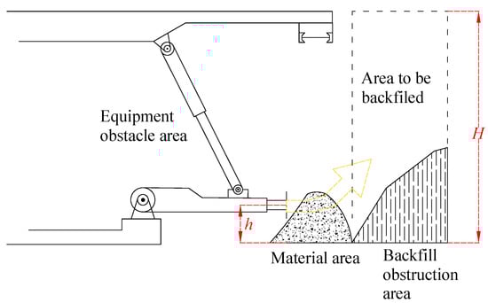
Figure 1.
Zoning of the solid backfilling workspace.
Herein, the height of the top plate within the current filling area is represented by H, while h denotes the height of the push plate in the given equation. In cases where l is a non-integer, the filling height is considered to be less than the height of a single filling to ensure the effectiveness of the top-of-the-filler filling body and maintain complementarity with respect to the topmost height.
To capture spatial and material information within the filling space, a three-dimensional coordinate system is established for the filling working surface, with the origin positioned at the midpoint of the upper top of the pushing mechanism of the filling bracket. The height of the filling material in the filling area is determined through laser scanning, which yields point cloud information relating to the filling material. Subsequently, information fusion techniques are employed to ascertain the filling material data [,,]. Furthermore, a fixed coordinate system is applied to the target points, allowing for seamless representation and mutual conversion of coordinates between the laser scanning and the filling space. For instance, ΨP denotes that the vector P is within the coordinate system , with the distance on each axis of ΨP serving as the projection of that vector on the corresponding axis.
As shown in the figure, the three-dimensional coordinate system is instantiated by three orthogonal unit vectors, and the point P is marked by a position vector indicated by arrows. Equivalently, ΨP can be considered to represent a position in three-dimensional space, or it can simply be denoted by an ordered set of three numbers. The components of the position vectors on each axis of the system are denoted by the subscripts x, y, and z, respectively:
The study utilizes a laser scanner for spatial scanning, with the scanner acting as the origin. The coordinates representing the scanner’s location are defined as a three-dimensional coordinate system, denoted as , for the purposes of this paper. In the following, we present the conversion formula between the and coordinate systems.
Herein, represent the vector distance from the origin of to the origin of , adjusting as the mount’s attitude changes.
2.2. Objective Function for Solid Backfilling Path Planning
The efficacy of filling in coal mines can be significantly influenced by a single filling trajectory and pushing path, making the conceptualization of an optimal push-press path scheme an urgent priority in this context. The primary focus of this paper is to conceptualize a suitable push-press path scheme for the filling stent push-press mechanism in coal mines. We aim to derive an optimal path that considers the steadiness requirement of the filling body, spatial and material constraints, and ensures the total filling material required is attained via the shortest path with minimum iterations. To achieve this, we propose a constraint-based position model for each path point and design an objective function that takes into account both the accumulation of material during the push-press process and the demand amount, as well as the shortest distance of the push-press path.
We delineate the path planning schema below:
Herein, the first term represents the difference between the amount of material sent and the amount of material to be sent, while the second term represents the contrast between the advanced path and the optimal path. represent the weights assigned to the two terms, such that . For this work, we set them both to 0.5. stands for the dimensional coordinate of the node of the th path; Q symbolizes the total amount of material required; and L defines the displacement from the starting point of the pusher plate to the target point.
2.3. Constraint Conditions
2.3.1. Volume Constraints on Path Planning
The stability of the mine’s roof and the internal pressure of the filling body are taken into account in the filling process when determining the volume of filling material needed at various densities. This calculation utilizes the compression ratio of the filling material, with the filling support’s push mechanism path being seen as effective in pushing the filling material as long as it remains below the filling drop interface. This is expressed as follows:
Herein, the required fallout volume is denoted by , with representing the bulk density of the fallout. indicates the filling area volume, and represents the density of the stabilized filling body.
2.3.2. Length Constraints on Path Planning
The path planning of filling equipment must prioritize the guarantee of the filling effect while also aiming for a shorter path length, resulting in reduced filling time and increased filling speed, ultimately leading to higher filling efficiency. To ensure the stability of the filling process, the path planning must ensure that the quantity of material passed is at least equal to the filling material needed for a single fill. Moreover, the path should be designed to accommodate the passing through void regions outside the material area, thus ensuring comprehensive coverage and fill precision.
Herein, represents the filling drop zone intersected by the path curve, while denotes the void zone crossed by the path curve. h and w represent the height and width of the pushing plate of the pushing mechanism, respectively.
2.4. The Penalty Function
The penalty function [] simplifies the process of finding a solution to the solid backfilling path planning problem by transforming the constrained problem into an unconstrained one, thus effectively facilitating the optimization process with respect to constraints. The penalty value is calculated as follows:
Herein, the numbers of inequality and equality constraints for path planning are denoted by N and H, respectively, with representing the penalty. The result of converting the initial n inequality constraints is signified by the function , while the result of converting the initial h equality constraints is represented by . The conversion of the inequality constraints is expressed as follows:
Furthermore, for the equality constraints in the H terms of the path planning problem, we represent their transformed format using , which transforms as follows:
The penalty function method can be utilized for optimization to address variables that exceed the range of the constraints. If a variable surpasses the limit designated by the inequality constraints, the penalty value is set to , while it is set to if it surpasses the limit set by the equality constraints. To strengthen the constraint, a larger positive integer, , can be used to multiply with the penalty value and added to the original objective function. This procedure results in an augmented function related to the original objective function.
The above equation implies that if a sufficiently large positive integer is chosen for , the objective function’s value will increase significantly when a variable exceeds the proposed constraints. This rapid increase aids in identifying this solution as non-optimal during the solution process. Therefore, it is essential to regulate the value of to strike a balance between the effects of the penalty value. A smaller provides more flexibility in managing the constraints and allows variables to slightly exceed the constraints, thereby expanding the potential solution space.
3. Adaptive Genetic-Particle Swarm Hybrid Algorithm Based on Path Planning for Solid Backfilling Mechanisms
3.1. Particle Swarm Optimization
The PSO is inspired by swarm intelligence, specifically simulating the foraging behavior of birds. In this model, each potential solution to an optimization problem is represented as a “particle” within the search space. These particles interact and share information to collectively identify the optimal solution. The particles are characterized by two key attributes—velocity and position—which are continuously adjusted to achieve the desired objective. The collaborative search for the optimal solution lies at the heart of the algorithmic approach [].
The position of a particle in the PSO corresponds to potential solutions, and its velocity reflects the direction and speed of movement in the solution space. By continually updating their velocity and position, particles undertake a search for the most optimized solution. In a D-dimensional search space containing n dimensionless particles, the position of the ith particle can be represented as follows:
Moreover, the velocity and direction of the ith particle’s flight are structured as follows:
The formula for adjusting particle velocity, as per Equation (13), is given by:
Furthermore, particles must adjust their positions in the iteration process, a process that can be represented by the formula in Equation (14).
In the context of PSO, the symbols and represent individual and global optimal values, respectively. The dynamics of particles learning from both their individual experiences and the experiences of the collective swarm are encapsulated by the terms and . These terms, also referred to as self-recognition and social recognition, are instrumental in shaping the learning process within the PSO framework.
The parameters and are random numbers drawn from the interval and are typically reduced in scale during the iterative process. The constants and are weights attached to individual and global extremes and are usually set to two in order to regulate the effects of such extremes. This regulation is crucial for effectively managing the impact of individual and global extremes in the iterative process.
During the iteration process, the weight coefficient of the particles decreases linearly, as shown in the following equation:
Herein, the state of the collective swarm continues to evolve as more iterations are performed, resulting in the continuous adjustment of particle positions. This is achieved through the progression of these positions according to the velocity and position updating formulas, which enables particles to iteratively converge towards the optimal solution. In this iterative process, is set to 0.9, to 0.4, is the maximum number of iterations, and k is the current iteration number. One of the key properties of the PSO algorithm is the iterative adjustment of particle positions, allowing for the ongoing refinement of the swarm’s state. This recurrent process continues until the aimed termination condition is fulfilled.
3.2. Genetic Algorithm
The genetic algorithm (GA) search process involves considering factors beyond the core information from the current population, including characteristics derived from accumulated experiences from previous iterations. Emulating natural selection, the process involves retaining and passing on exceptional characteristics of the population through processes such as crossover (hybridization), mutation, and other mechanisms characteristic of biological evolution. This iterative process aims to find the optimal solution in the global maximum, ultimately solving the problem at hand. The main process includes individual coding, population initialization, fitness evaluation, selection, crossover, mutation, and generation of a new population [].
3.2.1. Coding Design
This paper focuses on the application of genetic algorithms to problem-solving, which involves representing potential solutions as chromosomes. A chromosome, which consists of a chain of binary numbers, real numbers, or other symbols known as “genes”, is used to encode the solution. These chromosomes form a population that represents a set of potential solutions. The representation of solutions within genetic algorithms typically involves a specific coding strategy, such as binary encoding, real number encoding, or permutation encoding. Binary encoding is chosen as the primary form of coding in this paper due to its ease of management and its similarity to biological chromosome compositions.
3.2.2. Initializing Populations
The population initialization process in genetic algorithms usually begins with random generation, which is instrumental in creating initial individuals in the space of the solid backfilling mechanism route planning problem. This step is crucial as it sets the stage for the genetic algorithm optimization process. The size and distribution of the first population play a significant role in shaping the algorithm’s performance at this early stage. Mathematically, this can be denoted as follows:
3.2.3. Fitness Function
This paper designs the fitness function as a minimization objective function. The fitness function, represented as , is a quantifiable measurement of a solution’s quality. It is utilized to evaluate the strengths and weaknesses of individuals in a population, primarily based on an individual’s performance within the solution space to determine its fitness value. Proper design of the fitness function should accurately portray an individual’s performance, consequently influencing the convergence efficiency of the algorithm and the optimal solution discovery capability [].
Herein, the notation represents the minimum value of the function, and e is a small number chosen to ensure that the fitness function exceeds 0. Specifically, in this case, .
3.2.4. Selection Process
The selection operation is crucial as it serves to intensify the probability of the algorithm bypassing the locally optimal solution. This is achieved through the maintenance of a small proportion of the less well-adapted individuals, allowing them to participate in the offspring. Consequently, this facilitates the algorithm in discovering the globally optimal solution with higher chances. As a result, this selection process not only improves convergence speed but also enhances the quality of the results.
The stallion evolutionary algorithm, a variant of the evolutionary algorithm, enhances recombination by relying on individuals’ relative fitness values and selecting the best individuals (stallions) in each generation for recombination in order to maintain the population’s superior characteristics. This selection mechanism of the stallion algorithm reinforces the search efficiency of the genetic algorithm by strengthening the inheritance of the best individuals. The selection probability of individual in the stallion algorithm can be denoted as .
where N signifies the population size. The total fitness, S, is defined as:
The technique for selection from the populous involves opting for a population size denoted by M, which represents the number of individuals intended for selection into the next generation. After determining the population size, the next step is to compute the step size, denoted as , which is essential for the selection technique. The equation for calculating the step size is as follows:
The stallion evolution algorithm employs a detailed selection mechanism, as illustrated in Algorithm 1. Initially, a random number r is generated within the range , with the initial value set at 0. The selection process begins with the aim of identifying the first individual whose fitness value surpasses r. This is achieved by finding the smallest i that satisfies the condition . The selected individual then advances to the next generation, and r is subsequently increased by Step. This procedure is iterated exactly M times until the selected population consists of M individuals.
The final selection of individuals is mainly guided by the following formula:
Herein, the stallion evolution algorithm employs the fitness function to evaluate the fitness level of an individual X. This determines the likelihood of selection for a superior individual (stallion), with higher fitness levels correlating to a higher probability of being chosen as a stallion. This biased selectivity towards individuals with higher fitness levels allows for the progression of selected individuals to the next generation, where they participate in further evolutionary activities such as crossover and mutation operations. Despite the random nature of the selection mechanism, individuals with higher fitness levels are favored, ensuring diversity in the population and ultimately leading to the discovery of improved solutions.
| Algorithm 1 Stochastic universal sampling (SUS) mechanism. | |
| Require: | |
| Population size N | |
| Number of individuals to be selected M | |
| Fitness values array F, containing fitness values of N individuals | |
| Random number generation function rand() | |
| Ensure: | |
| Array of selected individual indices Selected, housing indices of M chosen individuals | |
| 1: procedure SUS() | |
| 2: | ▹Compute the total fitness |
| 3: | ▹Compute the step size |
| 4: | ▹ Generate an initial random number within the range |
| 5: | ▹ Initialize array for selected individuals |
| 6: for toM do | ▹ Initialize array for selected individuals |
| 7: | |
| 8: while do | |
| 9: | |
| 10: end while | ▹ Initialize array for selected individuals |
| 11: Add i to Selected | ▹ Incorporate the selected individual |
| 12: | ▹ Increase the random number for subsequent selection |
| 13: end for | |
| 14: return Selected | |
| 15: end procedure | |
3.2.5. Crossover and Mutation Operations
In genetic algorithms, crossover and mutation operations play a pivotal role, mirroring the chromosome crossover and gene mutation seen in biological inheritance. These operations are designed to amplify the diversity of the population as the genetic algorithm progresses through its search process, ultimately aiming to improve the algorithm’s ability to perform a local search. The probabilities of crossover and mutation serve as governing factors dictating the algorithm’s balance between exploration and exploitation, and in this paper, both values are set at 0.8.
- (1)
- Crossover Operation
The first step in the process involves selecting a parent individual. Following this, the next step is to ascertain the crossover point. In this study, binary encoding is used for the process. It assumes that if the length of the individual’s encoding is denoted as L, the intersection point may fall anywhere between 1 and . After determining the crossover point, one or more points within the encoding of the parent individual are arbitrarily chosen. The encoding of the two parent individuals is then assigned as follows:
If we denote the crossover point as k, the two new individuals, C and D, resulting from the crossover have the following coding:
At the crossover point, genetic information is exchanged between the parent individuals, resulting in the creation of a new individual.
- (2)
- Variant Operation
We start by analyzing the mutation operation represented by the function Mutate. Here, denotes the individual after mutation, and represents the selected individual from the current population for mutation, with denoting the mutation probability.
The mutation procedure consists of three stages. Initially, an individual is chosen from the existing population. Subsequently, one or more loci are randomly selected on the individual’s coding for the mutation. Finally, the genetic information of the selected locus or loci is modified, typically involving the conversion of a 0 to a 1 or a 1 to a 0 in a binary genetic code. Let us consider a scenario where the individual is chosen for mutation and the mutation locus is denoted as m. The coding for the mutated individual, denoted as F, can be expressed as:
Herein, the ¬ symbol indicates the negation operation, which involves flipping the binary value of the selected locus.
By using genetic operations such as crossover and mutation, the population generates a new set of individuals. Consequently, the genetic algorithm can explore the solution space and ultimately find the optimal solution.
3.2.6. The Recurring Process of the Algorithm
The entire algorithmic process can be recursively represented as:
Here, evolve denotes a combined process of selection, crossover, and mutation procedures.
3.3. Genetic-Particle Swarm Optimization
The proposed hybrid genetic-particle swarm optimization (GAPSO) algorithm is based on the architecture of the genetic algorithm (GA). By combining the benefits of both GA and PSO, the GAPSO algorithm seeks to enhance the efficiency and orientation of the population evolution. The genetic algorithm (GA) contributes to preserving population diversity and evolutionary capabilities through selection, crossover, and mutation procedures. On the other hand, the particle swarm optimization (PSO) helps guide the population toward the axiological direction of evolution, serving as an auxiliary mechanism within the algorithm.
The flow of the GAPSO algorithm is depicted in Figure 2. In the GAPSO model, the GA element plays a key role in maintaining the diversity of the population and guiding it towards superior individuals, achieved through chromosome selection and crossover operations. However, the evolution process may result in the degradation of certain individuals, disrupting the overall evolutionary process. To address this, the PSO is incorporated to optimize the evolutionary direction of these degraded individuals. This is achieved through continuous updates to the velocity and position of the particles, steering the degraded individuals back toward the optimization trajectory. The pseudocode for the GAPSO algorithm is presented in Algorithm 2.
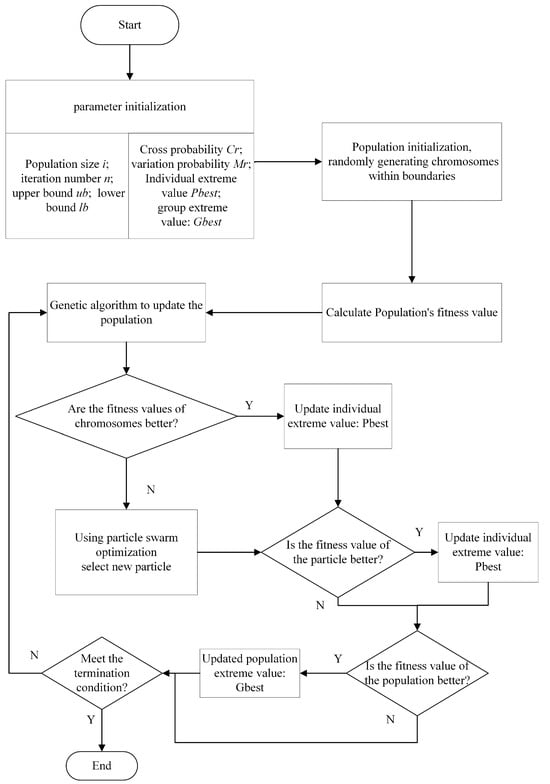
Figure 2.
Flowchart of the GAPSOS algorithm.
- (1).
- Initiate population.
- (2).
- Compute and store both the individual and population fitness values.
- (3).
- Use GA, which includes selection, crossover and mutation operations, to update the population. Amend the fitness value of particles and the population.
- (4).
- Assess individual degradation by computing the fitness value of all i individuals, . If , the i individual is regarded as degraded.
- (5).
- Employ the PSO to recalculate the fitness value by updating the location and velocity of any degraded individuals.
- (6).
- Determine if the fitness value refined by the PSO has improved; if so, update the fitness value.
- (7).
- Assess if the termination conditions have been achieved, i.e., if the maximum iteration count or the optimal population fitness value meets the threshold.
- (8).
- Repeat iteration: if termination condition(s) is not attained, return to step (3); otherwise terminate.
| Algorithm 2 GAPSO Algorithm. |
| Require: |
|
3.4. Adaptive Genetic-Particle Swarm Optimization
The computational process of solid-filling mechanism path planning somewhat mitigates the general limitations of GA and PSO algorithms. This section centers on the optimization of the hybrid algorithm in tandem with the specific path-planning process for solid-filling and propelling mechanism path planning. The algorithm’s optimization process for solid-filling and propelling mechanism path planning is the primary focus. Figure 3 illustrates the AGAPSO process.
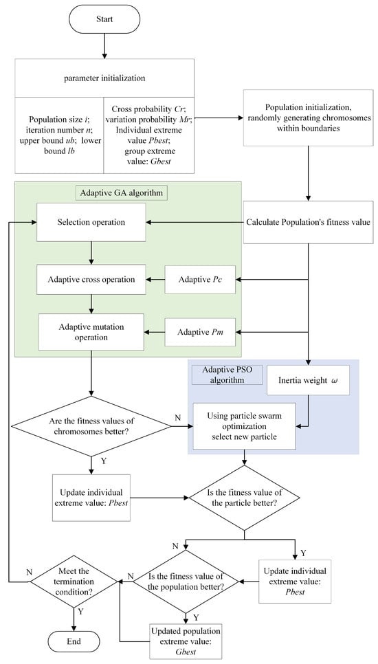
Figure 3.
Flowchart of the AGAPSOS algorithm.
The optimization of the genetic algorithm primarily revolves around adjusting the crossover probability and mutation probability, which directly impact the algorithm’s global evolutionary process. The crossover function plays a vital role in facilitating the emergence of highly-evolved individuals across different chromosomes, while the mutation operation is crucial for escaping local optima. On the other hand, the effectiveness of PSO is predominantly determined by the inertia weights. Specifically, larger inertia weights enhance the algorithm’s global search capabilities, while smaller weights strengthen its local search abilities. Therefore, fine-tuning the crossover probability, mutation probability of the genetic algorithm, and the inertia weight of the PSO is essential for enhancing the overall performance of the optimization algorithm.
This paper proposes a dynamic approach to setting crossover and mutation probabilities for particles in the genetic algorithm optimization phase. In traditional genetic algorithms, these probabilities are fixed values, resulting in all particles evolving at a uniform rate. This can lead to issues such as oscillations and slow convergence during the optimization process. By dynamically adjusting crossover and mutation probabilities according to each individual particle’s current state within the population, this adaptive evolution enhances the optimization performance of the genetic algorithm. Consequently, this approach facilitates rapid path planning for solid-filling equipment.
Initially, the fitness value of each particle is computed according to the attributes of the genetic algorithm and PSO. This paper utilizes the reciprocal of the objective function as the fitness function, with the minimum fitness value as the optimization goal. The fitness function expression is as follows:
Unearth the optimal fitness value :
The average fitness value is computed as:
According to Reference [], the optimal results in particle crossover probability range from 0.6 to 0.9. This means that when a particle’s fitness value exceeds the average, it is randomly selected within this probability range, ensuring the retention of the superior particles. On the other hand, when the fitness value is below the average, the crossover probability is set at 0.9, thus maximizing the opportunity for poorly performing particles to undergo crossover operations.
In this study, the crossover probability of particles is adjusted during iterative processes in accordance with the individual’s current fitness value, thus facilitating the effective retention of superior solutions throughout the optimization process of the genetic algorithm. Consequently, the setting of the crossover probability should duly consider the fitness value of particles, as it enhances the convergential capability and global search potential of the genetic algorithm. This strategy ensures the enhancement of the genetic algorithm’s ability to converge and its potential for global search.
Herein, represents the crossover probability of the current particle, with its maximum and minimum values denoted by and , respectively, set at 0.9 and 0.6. refers to the fitness of the current particle.
The mutation process plays a significant role in genetic algorithms by enabling the algorithm to break free from local optimal solutions. It achieves this by adjusting the mutation probability of a particle adaptively, consequently maintaining population diversity during later iterations and effectively improving its global search capability. To elaborate, increasing the mutation probability for particles with high fitness values allows the algorithm to explore new potential solution spaces, while decreasing it for particles with low fitness values focuses the algorithm on crossover and optimization processes to maintain the current search direction. In general, setting the mutation probability in the range of 0.01 to 0.1 is widely considered appropriate.
The adaptive mutation probability adjustment strategy helps maintain balance during the iterative process by promoting population diversity and effective utilization of excellent solutions. The mutation operation formula is defined as follows:
Herein, represents the current particle’s mutation probability, with its maximum and minimum values denoted by and , set at 0.1 and 0.01, respectively. Additionally, denotes the fitness of the current particle.
In the iterative process of a genetic algorithm, effectively optimizing the trajectory of a particle with a deteriorated fitness value can be achieved using the particle swarm optimization (PSO). To impart the PSO with adaptive adjustment capabilities, refining the inertia weights is crucial. The inertia weight (w) directly influences the direction and speed of optimization for the particles. Commonly oscillating between 0.4 and 0.95, the value of the inertia weight is adjustable according to the particle’s current adaptation value. The inertia weights can be dynamically described as follows: if a particle shows a commendable fitness value, indicating proximity to a potentially viable solution, its velocity can be curtailed for a more precise local search. Conversely, a particle with a low fitness value necessitates a broader search scope to discover a superior solution; thus, an increase in the particle’s velocity enhances its global search capability. Consequently, adjustments in the inertia weights can be dynamically set according to the particle’s current adaptation value and iteration number. In this study, the inertia weight will undergo updates as outlined. In the iterative process of a genetic algorithm, effectively optimizing the trajectory of a particle with a deteriorated fitness value can be achieved using the particle swarm optimization (PSO). To impart the PSO with adaptive adjustment capabilities, refining the inertia weights is crucial. The inertia weight (w) directly influences the direction and speed of optimization for the particles. Commonly oscillating between 0.4 and 0.95, the value of the inertia weight is adjustable according to the particle’s current adaptation value. The inertia weights can be dynamically described as follows: if a particle shows a commendable fitness value, indicating proximity to a potentially viable solution, its velocity can be curtailed for a more precise local search. Conversely, a particle with a low fitness value necessitates a broader search scope to discover a superior solution; thus, an increase in the particle’s velocity enhances its global search capability. Consequently, adjustments in the inertia weights can be dynamically set according to the particle’s current adaptation value and iteration number. In this study, the inertia weight will undergo updates as outlined.
Herein, the symbol represents the inertia weight, with and representing the maximum and minimum values, set at 0.95 and 0.4, respectively.
The above equations provide insights that suggest larger fitness values and higher inertia weights are advantageous for global search in the early stages of the algorithm. Conversely, during the later convergence stages, smaller fitness values and decreased inertia weights are more beneficial for a local search. Thus, the adaptive genetic-particle swarm optimization (AGAPSO) proposed in this study brings significant improvements to critical parameters within the GAPSO algorithm. The original fixed parameters transform into variable parameters that adapt to the particle population, leading to a substantial increase in algorithm variability. Consequently, the theoretical enhancement of particle optimization speed and precision is attained.
4. Algorithm Performance Test and Analysis
In this section, the path-planning model of the push-pressure mechanism is simulated using the AGAPSO algorithm to validate the algorithm’s feasibility in addressing path planning problems. Python, an interpreted high-level programming language, widely used in big data and artificial intelligence domains, is employed for this purpose due to its inherent strengths in algorithm editing. The experimental configuration encompasses 100 particles, a maximum of 300 iterations, and each particle comprises four features. The evaluation of the algorithm is based on the minimum adaptation value after iterations, the average value, and the number of iterations.
Upon closer examination of Figure 4, significant insights are revealed from the iterations of the three algorithms. It becomes apparent that AGAPSO exhibits superior convergence accuracy, as evidenced by its lower fitness value in comparison to both the single GA algorithm and the hybrid GAPSO. Additionally, the convergence speed analysis depicted in the figure illustrates that AGAPSO and GAPSO reach optimal solutions after approximately 5 iterations, while the GA algorithm requires around 15 iterations to achieve the same level of optimization. Consequently, the first two algorithms demonstrate faster convergence speed, thereby highlighting the effectiveness of AGAPSO and GAPSO in reaching optimal solutions more rapidly than the GA algorithm.
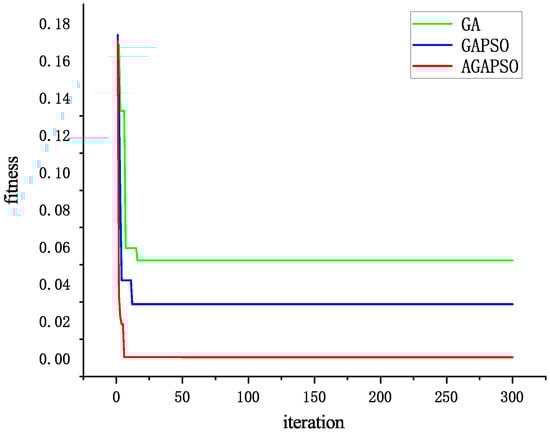
Figure 4.
Iteration effect diagrams for the three algorithms.
The statistical metrics data of the algorithm optimization for the solid filling mechanism path planning problem are presented in Table 1, demonstrating the performance comparison among three algorithms: AGAPSO, GAPSO, and GA. Examination of the overall effectiveness reveals that the AGAPSO algorithm outperforms the GAPSO and GA algorithms, as illustrated in the figures above. Specifically, the maximum, minimum, D-value (difference between maximum and minimum), and average values of AGAPSO are significantly lower than those of GAPSO and GA. Notably, the minimum value of AGAPSO (6.28 × 10⁻⁴) is notably lower than that of GAPSO (2.88 × 10⁻²) and GA (2.88 × 10⁻²). This significant difference suggests that AGAPSO demonstrates superior performance in the best-case scenario. Furthermore, the D-value of AGAPSO (6.90 × 10⁻³) is notably lower than that of GAPSO (5.90 × 10⁻²) and GA (1.15 × 10⁻¹), indicating that the results of the AGAPSO algorithm exhibit higher stability and lower volatility. Additionally, the average value of AGAPSO (3.64 × 10⁻³) is noticeably lower than that of GAPSO (5.26 × 10⁻²) and GA (8.01 × 10⁻²), underscoring its superior average performance compared to the other two algorithms.

Table 1.
Comparison of algorithm performance.
To better illustrate the superiority of AGAPSO over GAPSO and GA algorithms, we calculate the percentage improvement for each metric.
- (1)
- Minimum value:
AGAPSO improves the minimum value compared to GAPSO.
AGAPSO improves the minimum value compared to GA:
- (2)
- D-value (stability):
AGAPSO has increased D-value compared to GAPSO:
The D-value of AGAPSO compared to GA was increased by:
- (3)
- Average values:
AGAPSO improves the mean value compared to GAPSO:
AGAPSO improves the mean value compared to GA:
Based on the above calculations, it is evident that AGAPSO demonstrates substantial improvement in comparison to GAPSO and GA across various metrics, including minimum, D-value, and average performance. In particular, AGAPSO exhibits an improvement of nearly 98% in the minimum value, signifying its superior performance at the optimal level compared to the other two algorithms. Furthermore, AGAPSO showcases improvements ranging from approximately 88% to 94% in terms of stability (D-value) and 93% to 95% in average performance, underscoring its significant superiority in these aspects. This analysis indicates that AGAPSO offers a more comprehensive evaluation and superior optimization-seeking performance in the context of path planning for the push-press mechanism.
5. Model Simulation Experiment and Analysis
This section utilizes the AGAPSO algorithm proposed in this paper to compute the path planning model for the solid backfilling push-press mechanism. Concurrently, a comparative analysis is conducted with the GA algorithm and the GAPSO algorithm, focusing on observing the convergence states of the three optimization algorithms. Subsequently, the planning of the filling environment in real-life scenarios is analyzed to evaluate the pushing efficiency and stability. This approach is employed to confirm the superiority of the AGAPSO algorithm in the context of the solid backfilling stent pushing mechanism.
5.1. Model Simulation Experiment
The improved algorithms are verified for their practicability and superiority by utilizing the spatial state of the actual mining airspace and the fallout model to plan the push-pressure path and comparing the three algorithms as well as the filling efficiency in the case of the fill-push pressure.
Section 2.1 discusses the state space of the air-mining zone. To evaluate the effectiveness and accuracy of the presented algorithms, a series of simulation experiments were conducted with a focus on the tamping trajectory of the solid backfilling face within a coal mine. The simulations replicated the working face of a mine with an average mining height of 800 mm, along with the incorporation of a corresponding hydraulic bracket measuring 1500 mm in width. Furthermore, the components of the bracket, including the gangue blocking plate and the push solid plate, were designed to measure 1500 mm in width and 200 mm in height.
For the purpose of this study, it was assumed that shifts of 1000 mm would be made, although the bracket was designed to accommodate single shifts within the range of 500–1000 mm. The initial planning consideration focused on filling the existing hollows, taking into account the mining height and the height of the push-pressure mechanism. As a result, the area was divided into four distinct layers, which required four stages of fill. The center position of the filling push-pressure mechanism was established as the origin (0, 600, 200). It was acknowledged that the bi-dimensional nature of the filling operation allowed for the process to be conceptualized within a two-dimensional space.
The reference point for accurately representing the position of the push plate within the filling area and ensuring complete submersion of the push mechanism within the material was determined as the top vertex of the centralized push plate. Following this, a series of target coordinates were established, mapping the intended movement of the pushing mechanism from the origin (0, 0) to the nodes (1000, 600, 200), (1000, 600, 400), (1000, 600, 600), and finally (1000, 600, 800).
The scraper transporter, filling support, and filling roof and floor were recognized as obstacles in this process. The surface state of the filling drop was assessed using a surface function in the following formula.
The equation contains several key parameters: the symbol represents the height of the surface center, while the ratio captures the surface’s slope. Additionally, the parameter refers to the overall height of the surface. Meanwhile, the symbols , , and denote the horizontal coordinate, vertical coordinate, and degree of prominence of the surface center, respectively.
The enhanced algorithm proposed above will be validated through the presentation of four experimental scenarios designed to replicate real operating contexts. These scenarios aim to achieve four different objectives pertaining to the search for filling paths. Each scenario will be comprised of three experiment sets that compare the search paths of the traditional genetic algorithm (GA), genetic algorithm particle swarm optimization (GAPSO), and assisted ga particle swarm optimization (AGAPSO) algorithms.
The initial nodes are represented by the green nodes on the left side of the three-dimensional coordinate system, as illustrated in Figure 5, while the target nodes are depicted by the blue nodes on the right. These target nodes are further categorized into goal 1, goal 2, goal 3, and goal 4 based on their respective heights. The experimental results are visually depicted in Figure 6, Figure 7, Figure 8 and Figure 9. The positioning and shape of the fill dropping are identified by the black pattern, the search paths of the GA algorithm are represented by the light green lines, while the search paths of the GAPSO algorithm are denoted by the blue lines. Additionally, the final path discovered by the AGAPSO algorithm is indicated by the red lines.
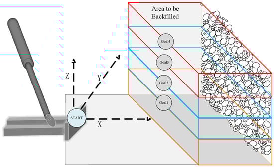
Figure 5.
Schematic of filling environment and target.
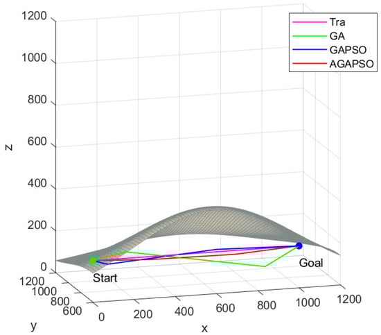
Figure 6.
Pathway planning chart for goal 1.
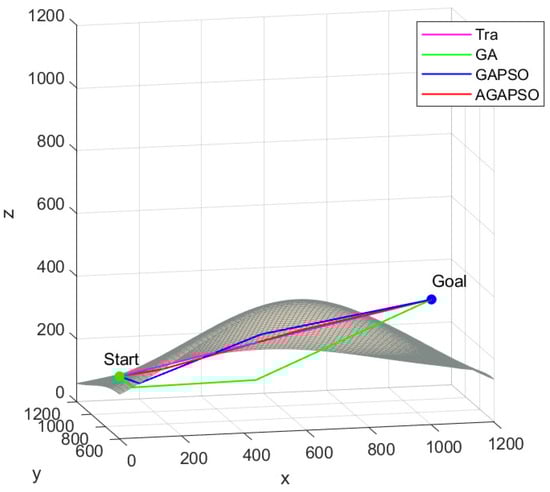
Figure 7.
Pathway planning chart for goal 2.
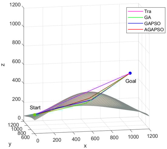
Figure 8.
Pathway planning chart for goal 3.
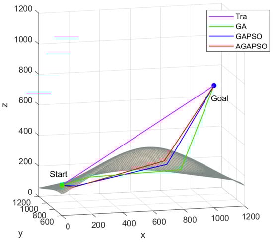
Figure 9.
Pathway planning chart for goal 4.
The traditional push-pressing method involves pushing the material directly from the starting point to the target point. This approach is simple and theoretically the most efficient. However, when the target point is higher, the material needs to be dropped several times, ultimately affecting filling efficiency. When comparing the paths calculated by various algorithms, it is observed that the path determined by the AGAPSO algorithm closely approximates the theoretical optimal path. For target two, the material demand exceeds what can be pushed directly by the push-press path due to an increased blank area from the material surface to the target point. Consequently, the optimized path of the AGAPSO algorithm deviates slightly from the traditional path, while the paths optimized by the GA and GAPSO algorithms exhibit larger offsets. As for objectives three and four, the traditional push-press method fails to fulfill the filling requirements, necessitating additional material dropping to achieve the desired filling material height. This inadvertently diminishes filling efficiency. Figure 3 and Figure 4 illustrate that in order to meet the filling material demand, the algorithm-optimized path traverses a portion of the distance within the filling material, enabling the pushing and pressing of the material.
5.2. Analysis of Filling Effect
To assess the state of the filling material before and after the execution of the algorithms, 100 simulations are carried out for each experiment. Subsequently, the outcomes are evaluated based on key metrics, including calculation time, path length, amount of material, and overall efficiency. These parameters are then quantified to derive the average values, which are subsequently compared to ascertain the efficacy of the filling paths associated with the three algorithms. The comparison results are detailed in Table 2.
Table 2.
Comparison of the specified filling targets with the corresponding algorithm performance.
The redundancy in material k is related to the required material quantity and the actual material quantity used through the following equation:
A smaller value of k means that the actual amount of material used is closer to the required amount, which improves filling effectiveness. Conversely, a larger value of k indicates less efficient filling.
The paper adopts the traditional push-press method of filling as the standard of reference, as the effectiveness of the filling process is directly proportional to the speed of the action, and the speed is influenced by the length of the push-press route. Thus, for a more efficient process, shorter routes are preferred. To measure the efficiency of route planning, the path’s actual growth rate d is utilized as a parameter, as identified by the following equation:
Herein, represents the path lengths computed by various algorithms, and stands for the path lengths obtained from traditional algorithms.
This paper presents a comparative analysis of the filling results before and after path planning for various filling targets using simulated data. Analysis of the table reveals that an increase in the target node height results in a corresponding rise in the material demand, driven by the voiding zone between the heights of the material filling targets. In terms of calculation time, the traditional pushing method generally requires minimal computation time and primarily involves identifying the target node. However, as the height of the pushing target increases, the traditional pushing method struggles to accomplish the pushing target in a single instance due to the increasing complexity of the algorithm, consequently leading to an increase in the algorithm’s computation time. Nonetheless, in comparison with the GAPSO algorithm, the AGAPSO algorithm’s computation time only sees a marginal increase of 0.03 s. Given the primary goal of ensuring a robust filling effect and efficiency, this slight increase in computation time is not significant.
As shown in Figure 10, a comparison of the GA and GAPSO algorithms demonstrates that the AGAPSO algorithm calculates the smallest path growth rate d for both, indicating that it adheres most closely to the shortest path.
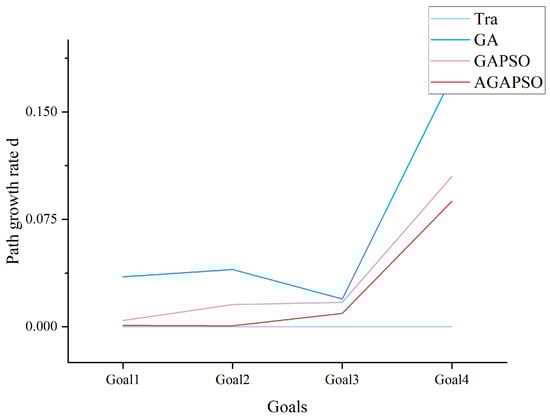
Figure 10.
Schematic comparison of the growth ratio of the algorithm-optimized paths under four objectives.
Figure 11 demonstrates that the GAPSO algorithm, which is proposed in this paper, has the lowest material redundancy among the four filling objectives, indicating that it best meets the material requirements.
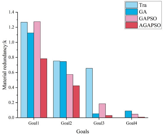
Figure 11.
Comparison of the material redundancy ratios of different algorithms for the four objectives.
The comparison of GAPSO and GA optimization based on precision is presented in Table 3. The results reveal that AGAPSO optimization led to a substantial improvement in accuracy during lower-level of planning objectives, with enhancements of 27.57% and 19.16%, respectively. Furthermore, accuracy was also notably enhanced at the highest level planning objectives, showing an improvement of 3.78% and 8.11%. When taking into account both the quantity of material and path length, it is apparent that the path length and material volume, as calculated by the AGAPSOA algorithm, more closely align with the expected material requirement. This finding aligns with the design goals of the paper’s path planning.
Table 3.
Accuracy improvement performance of AGAPSO over other algorithms for filling route planning.
6. Discussion
The purpose of this study is to propose an optimization method for the path planning of solid backfill propulsion machinery in coal mines, the adaptive genetic-particle swarm optimization algorithm (AGAPSO). Our research questions focus on how to improve the efficiency and accuracy of path planning through algorithmic optimization.
Through method selection and detailed data analysis, we find that the AGAPSO algorithm has made significant progress in integrating the advantages of global search capability and local search, and has achieved higher filling efficiency and safety in coal mine solid backfill operations. Our research results not only theoretically enrich the research field of solid backfill propulsion mechanical path planning but also provide a more efficient solution in practical applications.
Specifically, in our experiments, AGAPSO achieved an average convergence speed that was approximately three times faster than the base GA algorithm. In terms of accuracy, the AGAPSO algorithm attained a lower fitness value, indicating enhanced convergence, by approximately 88% compared to GA and 94% compared to GAPSO. Moreover, the reduction in path length and material redundancy was substantial. AGAPSO showed a 27.57% improvement in optimization efficiency over the GA algorithm alone and a 19.16% improvement over the improved GAPSO algorithm.
AGAPSO demonstrates marked improvements in convergence speed and accuracy, underscoring the critical importance of integrating global and local search capabilities. Moreover, the substantial advancements of AGAPSO in reducing path length and material redundancy further substantiate its potential utility in enhancing the safety and economic feasibility of solid backfilling in coal mines.
While the AGAPSO algorithm exhibits theoretical potential and practical advantages, it is essential to acknowledge that its real-world application might be constrained by the need for sophisticated hardware and accurate environmental data. Additionally, the representation of the coal mine environment in our samples may not fully encapsulate the complexity of real-world conditions. This limitation underlines the necessity for extensive empirical testing and validation of the algorithm in diverse and complex mining conditions to ensure its robustness and reliability.
Future research should prioritize enhancing the adaptability and efficiency of the AGAPSO algorithm in varied mining environments. This endeavor could involve detailed empirical testing across different mining conditions, using the data gleaned from such tests to fine-tune the algorithm. For example, integrating advanced optimization strategies like deep learning and reinforcement learning could potentially amplify the algorithm’s performance, as suggested by the substantial improvements observed in our study.
Furthermore, integrating AGAPSO with mine filling systems, monitoring systems, and automation equipment can significantly augment operational efficiency. This integration should be backed by a data-driven approach, where insights from real-world applications of AGAPSO inform the continuous refinement and optimization of the system.
Ensuring environmental protection and operational safety remains paramount. Future research should leverage the data from AGAPSO’s applications to bolster these aspects, ensuring that the development of filling technology remains both sustainable and efficient.
Through a meticulous data-driven approach, we aim to further substantiate the theoretical and practical contributions of AGAPSO, paving the way for its broader application and continuous enhancement in the field of coal mine solid backfilling.
7. Conclusions
This study proposes an optimization method, adaptive genetic-particle swarm optimization (AGAPSO), a novel approach designed to optimize path planning for coal mine solid backfilling and pushing mechanisms. The research addresses the critical need for enhanced efficiency and precision in path planning within the complex and dynamic environments of coal mines. The AGAPSO algorithm integrates the powerful global search capability of GA and the local search advantage of PSO, which fills the gap of coal mine solid backfill path planning research.
Our meticulous analysis and comparative studies highlight the superior performance of AGAPSO. The algorithm not only expedites the convergence process but also ensures higher precision in path planning compared to its counterparts. Specifically, AGAPSO exhibits a three-fold improvement in convergence speed over the base GA algorithm and a significant enhancement in stability and average performance by approximately 88% to 94%. These performance metrics underscore the algorithm’s potential to revolutionize path planning in coal mine solid backfilling, offering substantial improvements in operational efficiency and safety.
Its ability to optimize path length and reduce material redundancy by substantial margins (27.57% over GA and 19.16% over GAPSO) not only demonstrates its superiority in theoretical models but also signifies its potential in practical applications. These improvements bear profound implications for the safety, economic viability, and environmental sustainability of coal mine solid backfilling operations.
Looking forward, the AGAPSO algorithm opens new avenues for research and application. Its adaptability and efficiency in complex mining environments, coupled with its integration potential with monitoring systems and automation equipment, set the stage for a new era of intelligent mining operations. The AGAPSO algorithm’s significant performance enhancements and adaptability pave the way for safer, more efficient, and environmentally responsible mining practices.
In conclusion, the AGAPSO algorithm stands as a testament to innovative research and development in the field of mining operations. Its superior performance, significant improvements in operational efficiency, and potential for broad application underscore its importance as a groundbreaking contribution to the field. As we continue to refine and adapt this novel algorithm, we anticipate a future where mining operations are not only safer and more efficient but also more harmonious with the environmental and economic frameworks they operate within.
Author Contributions
Conceptualization, Y.L. and Z.Z.; methodology, Y.L. and Z.Z.; software, Z.Z.; validation, L.B. and Y.W. (Yiying Wang); formal analysis, L.B. and Y.W. (Yanwen Wang); investigation, L.B. and S.Y.; resources, Y.L.; data curation, Z.Z.; writing—original draft preparation, L.B., Z.Z., X.Z. and S.Y.; writing—review and editing, L.B., Z.Z., X.Z. and S.Y.; visualization, L.B.; supervision, L.B.; project administration, Y.L. and Y.W. (Yanwen Wang) and L.B.; funding acquisition, Y.L. and Y.W. (Yiying Wang). All authors have read and agreed to the published version of the manuscript.
Funding
This research was funded by the Hebei Provincial Natural Science Foundation Project (E2020402064).
Institutional Review Board Statement
Not applicable.
Informed Consent Statement
Not applicable.
Data Availability Statement
The raw data supporting the conclusions of this article will be made available by the authors upon request.
Conflicts of Interest
The authors declare no conflicts of interest.
References
- Zhang, J.; Tu, S.; Cao, Y.; Tan, Y.; Xin, H.; Pang, J. Research progress in underground intelligent sorting and in-situ filling technology for deep coal mines. J. Min. Saf. Eng. 2020, 37, 1–10+22. [Google Scholar]
- Liu, J.; Bi, J.; Zhao, L.; Xie, G. Research and application on automatic control of comprehensive mechanized solid backfill coal mining. Coal Sci. Technol. 2016, 44, 149–156. [Google Scholar]
- Zhang, P.; Li, F.; Zhu, H.; Niu, H.; Li, X. Statistical analysis and prevention countermeasures of coal mine accidents from 2008 to 2020. Min. Saf. Environ. Prot. 2022, 49, 128–134. [Google Scholar]
- Miao, X. Progress of fully mechanized mining with solid backfilling technology. J. China Coal Soc. 2012, 37, 1247–1255. [Google Scholar]
- Li, J.; Kou, Y.; Yang, Z.; Wang, S. Summary of research status of `three under’ coal filling mining. Sci. Technol. Innov. 2012, 12, 43–44. [Google Scholar]
- Wang, G.; Wang, H.; Ren, H.W.; Zhao, G.R. Scenario objectives and development path of smart coal mine 2025. J. China Coal Soc. 2018, 43, 295–305. [Google Scholar]
- Liu, J.; Li, X.; He, T. Current status and development of backfill mining in China. J. Coal Sci. Eng. 2020, 26, 141–150. [Google Scholar]
- Zhang, J.; Miao, X.; Guo, G. Development Status of Backfilling Technology Using Raw Waste in Coal Mining. J. Min. Saf. Eng. 2009, 26, 7. [Google Scholar]
- Liu, J. Research and Application of Kilometer Deep Well Filling Mining Technology and Equipment. Coal Sci. Technol. 2013, 41, 5. [Google Scholar]
- Bo, L.; Yang, S.; Liu, Y.; Zhang, Z.; Wang, Y.; Wang, Y. Coal Mine Solid Waste Backfill Process in China: Current Status and Challenges. Sustainability 2023, 15, 13489. [Google Scholar] [CrossRef]
- Liu, J.; Zhao, Q. Coal Mining by Coal Filling; Coal Industry Press: Beijing, China, 2011. [Google Scholar]
- Gao, H.; Zhao, L.; Du, X.; Yuan, W. Research and design of multi-hole bottom discharge filling scraper conveyor. Coal Mine Mach. 2014, 6, 131–133. [Google Scholar] [CrossRef]
- Wei, G.; Li, Y. Superstatic filling hydraulic support structure. Coal Mine Mach. 2015, 36, 2. [Google Scholar]
- Bo, L.; Yang, S.; Liu, Y.; Wang, Y.; Zhang, Z. Research on the data validity of a coal mine solid backfill working face sensing system based on an improved transformer. Sci. Rep. 2023, 13, 11092. [Google Scholar] [CrossRef] [PubMed]
- Zhang, Q.; Zhang, J.; Wu, X.; Huang, Y.; Zhou, N. Research on the reasonable tamping distance from the top of the hydraulic support for solid-filled coal mining. J. Coal 2013, 38, 6. [Google Scholar]
- Yan, S.; Shi, Y.; Wang, H.; Wang, Y. Experimental Research and Application of Solid Filling Cementitious Materials. Coal Eng. 2022, 3, 54. [Google Scholar]
- Russell, S.J.; Norvig, P. Artificial Intelligence a Modern Approach; Pearson: London, UK, 2010. [Google Scholar]
- Deng, Y.; Chen, Y.; Zhang, Y.; Mahadevan, S. Fuzzy Dijkstra algorithm for shortest path problem under uncertain environment. Appl. Soft Comput. 2012, 12, 1231–1237. [Google Scholar] [CrossRef]
- Zong, T.; Li, F.; Zhang, Q.; Sun, Z.; Lv, H. Autonomous Process Execution Control Algorithms of Solid Intelligent Backfilling Technology: Development and Numerical Testing. Appl. Sci. 2023, 13, 11704. [Google Scholar] [CrossRef]
- Li, F.; Da Xu, L.; Jin, C.; Wang, H. Intelligent bionic genetic algorithm (IB-GA) and its convergence. Expert Syst. Appl. 2011, 38, 8804–8811. [Google Scholar] [CrossRef]
- Liu, Y.; Wang, C.; Wu, H.; Wei, Y.; Ren, M.; Zhao, C. Improved LiDAR Localization Method for Mobile Robots Based on Multi-Sensing. Remote Sens. 2022, 14, 6133. [Google Scholar] [CrossRef]
- Dorigo, M.; Birattari, M.; Stutzle, T. Ant colony optimization. IEEE Comput. Intell. Mag. 2006, 1, 28–39. [Google Scholar] [CrossRef]
- Mirjalili, S.; Mirjalili, S. Genetic algorithm. In Evolutionary Algorithms and Neural Networks: Theory and Applications; Springer: Berlin/Heidelberg, Germany, 2019; pp. 43–55. [Google Scholar]
- Huang, Y. Advances in artificial neural networks—Methodological development and application. Algorithms 2009, 2, 973–1007. [Google Scholar] [CrossRef]
- Schutte, J.F.; Reinbolt, J.A.; Fregly, B.J.; Haftka, R.T.; George, A.D. Parallel global optimization with the particle swarm algorithm. Int. J. Numer. Methods Eng. 2004, 61, 2296–2315. [Google Scholar] [CrossRef]
- Naderi, K.; Rajamäki, J.; Hämäläinen, P. RT-RRT* a real-time path planning algorithm based on RRT. In Proceedings of the 8th ACM SIGGRAPH Conference on Motion in Games, Paris, France, 16–18 November 2015; pp. 113–118. [Google Scholar]
- Zhao, Y.; Zheng, Z.; Liu, Y. Survey on computational-intelligence-based UAV path planning. Knowl.-Based Syst. 2018, 158, 54–64. [Google Scholar] [CrossRef]
- Xu, J.; Huang, Y. Path Planning of Robot in Coal Mine Using Genetic Membrane Algorithms. In Proceedings of the 2nd International Conference on Information Technologies and Electrical Engineering, Zhuzhou, China, 6–7 December 2019; pp. 1–5. [Google Scholar] [CrossRef]
- Cui, S.G.; Dong, J.l. Detecting Robots Path Planning Based on Improved Genetic Algorithm. In Proceedings of the 2013 Third International Conference on Instrumentation, Measurement, Computer, Communication and Control, Shenyang, China, 21–23 September 2013; pp. 204–207. [Google Scholar] [CrossRef]
- Quan, G.; Tan, C.; Hou, H.; Wang, Z. Cutting path planning of coal shearer base on particle swarm triple spline optimization. Coal Sci. Technol. 2011, 39, 77–79. [Google Scholar]
- Wang, S.; Ma, D.; Ren, Z.; Qu, Y.; Wu, M. Study on Method of Cutting Trajectory Planning Based on Improved Particle Swarm Optimization for Roadheader. In Advances in Swarm Intelligence, Proceedings of the 10th International Conference, ICSI 2019, Chiang Mai, Thailand, 26–30 July 2019; Springer: Berlin/Heidelberg, Germany, 2019; pp. 167–176. [Google Scholar]
- Wang, X.; Shi, Y.; Ding, D.; Gu, X. Double global optimum genetic algorithm–particle swarm optimization-based welding robot path planning. Eng. Optim. 2016, 48, 299–316. [Google Scholar] [CrossRef]
- Tong, Y.; Zhong, M.; Li, J.; Li, D.; Wang, Y. Research on intelligent welding robot path optimization based on GA and PSO algorithms. IEEE Access 2018, 6, 65397–65404. [Google Scholar] [CrossRef]
- Wang, X.C.; Yue, X.G. Algorithm of coal mine rescue robot model based on PSO and GEP. Appl. Mech. Mater. 2013, 416, 739–742. [Google Scholar] [CrossRef]
- Jiao, S.; Liu, J.; Shang, L. Backfill automation system of comprehensive mechanized solid backfill coal mining. Coal Sci. Technol. 2015, 43, 109–113. [Google Scholar]
- Wang, X.; Huang, X.; Bian, F.; Sun, J. 3D triangulation of terrestrial laser scanning data based on spherical projection. In Proceedings of the Geoinformatics 2007: Cartographic Theory and Models, Nanjing, China, 25–27 May 2007; SPIE: Bellingham, WA, USA, 2007; Volume 6751, pp. 59–67. [Google Scholar]
- Monsalve, J.J.; Baggett, J.; Bishop, R.; Ripepi, N. Application of laser scanning for rock mass characterization and discrete fracture network generation in an underground limestone mine. Int. J. Min. Sci. Technol. 2019, 29, 131–137. [Google Scholar] [CrossRef]
- Jiang, Q.; Shi, Y.E.; Yan, F.; Zheng, H.; Kou, Y.Y.; He, B.G. Reconstitution method for tunnel spatiotemporal deformation based on 3D laser scanning technology and corresponding instability warning. Eng. Fail. Anal. 2021, 125, 105391. [Google Scholar] [CrossRef]
- Dolgopolik, M.V. Smooth exact penalty functions II: A reduction to standard exact penalty functions. Optim. Lett. 2016, 10, 1541–1560. [Google Scholar] [CrossRef]
- Mohamed, K.S. Bio-Inspired Machine Learning Algorithm: Genetic Algorithm. In Machine Learning for Model Order Reduction; Springer International Publishing: Cham, Switzerland, 2018; pp. 19–34. [Google Scholar]
- Yang, H.; Su, M.; Wang, X.; Gu, J.; Cai, X. Particle sizing with improved genetic algorithm by ultrasound attenuation spectroscopy. Powder Technol. 2016, 304, 20–26. [Google Scholar] [CrossRef]
Disclaimer/Publisher’s Note: The statements, opinions and data contained in all publications are solely those of the individual author(s) and contributor(s) and not of MDPI and/or the editor(s). MDPI and/or the editor(s) disclaim responsibility for any injury to people or property resulting from any ideas, methods, instructions or products referred to in the content. |
© 2024 by the authors. Licensee MDPI, Basel, Switzerland. This article is an open access article distributed under the terms and conditions of the Creative Commons Attribution (CC BY) license (https://creativecommons.org/licenses/by/4.0/).