Analysis of Meshfree Galerkin Methods Based on Moving Least Squares and Local Maximum-Entropy Approximation Schemes

Abstract

Over the last two decades, meshfree Galerkin methods have become increasingly popular in solid and fluid mechanics applications. A variety of these methods have been developed, each incorporating unique meshfree approximation schemes to enhance their performance. In this study, we examine the application of the Moving Least Squares and Local Maximum-Entropy (LME) approximations within the framework of Optimal Transportation Meshfree for solving Galerkin boundary-value problems. We focus on how the choice of basis order and the non-negativity, as well as the weak Kronecker-delta properties of shape functions, influence the performance of numerical solutions. Through comparative numerical experiments, we evaluate the efficiency, accuracy, and capabilities of these two approximation schemes. The decision to use one method over the other often hinges on factors like computational efficiency and resource management, underscoring the importance of carefully considering the specific attributes of the data and the intrinsic nature of the problem being addressed.

1. Introduction

Over the past few decades, conventional grid-based numerical methods have been well-developed and successfully applied to a wide variety of boundary value problems in engineering and applied science. Despite their numerical advantages and great success, grid-dependent methods face inherent difficulties in various aspects when employed to solve large-deformation problems. In response to these challenges, a myriad of meshfree methods have emerged as powerful numerical techniques. These methods aim to mitigate certain issues by constructing the approximation of unknowns based on scattered points without relying on fixed mesh connectivity. Related reviews of meshfree methods may be found in [1,2,3].

Notable examples of meshfree methods encompass Smoothed Particle Hydrodynamics (SPH) [4,5,6], Element-Free Galerkin (EFG) [7,8], Reproducing Kernel Particle Method (RKPM) [9], Material Point Method (MPM) [10,11], Natural Element Method (NEM) [12,13,14] and Optimal Transportation Meshfree (OTM) [15,16]. Despite their diversity, meshfree methods can be categorized based on the approximation schemes employed to construct compactly supported shape functions. The spectrum of meshfree approximation schemes include geometry-based approximation, such as natural neighbour interpolation, kernel estimates, as well as optimization-based schemes including moving least squares and maximum-entropy approximation.

The concept of kernel estimates (KE), introduced in [4,5], forms the basis for SPH. The kernel function used in this process serves the same role as the test function in Galerkin methods. Despite the zeroth-order completeness of SPH’s continuous form and the high-order consistency of most kernel functions, discrete SPH struggles to reproduce constant fields on irregular node sets. As a result, numerous improvements have been made to fulfill the completeness, such as Johnson-Beissel correction [17], Randles-Libersky correction [18], Krongauz-Belytschko correction [19], Monaghan’s symmetrization on derivative approximation [20], etc. However, the SPH shape functions are still non-interpolant and do not verify the Kronecker-delta property. Under these circumstances, the imposition of Dirichlet boundary conditions proves to be more challenging in meshfree methods compared to the finite element method.

Moving Least Squares (MLS) serves as a method for attaining high-accuracy approximations based on specified nodes within a domain, initially proposed by Lancaster and Salkauskas [21] for curve and surface fitting. After its successful application in solid mechanics, notably in the Diffuse Element Method (DEM) introduced by Nayroles et al. [22], MLS has been integrated into various meshfree techniques, including SPH [23], RKPM [24] and the Immersed Boundary Method (IBM) [25]. MLS typically employs a polynomial basis to meet consistency conditions: any consistency order can be reached provided the order of the polynomial basis is high enough. Nevertheless, the utilization of a high-order polynomial basis introduces potential challenges, such as the negativity of shape functions. In addition, similarly to SPH, MLS lacks satisfaction of the Kronecker-delta property along boundaries. The efficient imposition of essential boundary conditions in Galerkin-based meshfree methods remains a challenge.

The approximation scheme used in NEM, where elements are defined based on the natural connectivity of nodes, is referred to as natural neighbour (NN) interpolation. It constructs interpolants based on the natural neighbour coordinates, drawing from foundational works by Sibson [26,27] and Belikov [28,29]. Following the application of NEM to elliptic boundary value problems in solid mechanics by Sukumar [13], Chinesta et al. further extended NEM to structural and process simulations [30]. While NEM demonstrates remarkable completeness and accuracy, as validated by Sukumar [31], it does entail a substantial computational cost, particularly for Sibson interpolation. An analysis, made by Alfaro et al. [32], showed that Sibson interpolation demands computational efforts several orders of magnitude greater than traditional piecewise polynomial interpolation in finite elements. However, in the realm of nonlinear computations, where frequent Newton-Raphson iterations are essential, the relative cost of calculating the interpolants becomes less prominent in comparison to the computational load associated with updating the tangent stiffness matrix.

More recently, there has been a growing interest in maximum-entropy (max-ent) approximation schemes within the category of meshfree particle methods. In Sukumar’s original work [33], max-ent approximation is applied to polygonally-shaped simplices in order to circumvent the challenges associated with full matrices. Successive research on the robustness, efficiency, and versatility of the max-ent approximation scheme include but are not limited to the convergence analysis [34], the automatic adaptation of support size [35], and higher-order consistency max-ent schemes [36].

Leveraging the principles of the maximum-entropy and delaunay triangulation, Arroyo and Ortiz [37] proposed the Local Maximum-Entropy (LME) approximation scheme as a statistical inference problem, incorporating the positivity and consistency requirements as constraints. This scheme bears similarities with those obtained from MLS, but possesses the weak Kronecker-delta property at the boundary, which allows the direct imposition of essential boundary conditions. Hence, the LME approximation has demonstrated its accuracy and stability in dealing with problems involving large deformation and phase transition when employed as shape functions. Additionally, the LME approximation is incorporated in constructing the surrogate models for structural reliability analysis, offering an accurate and robust approach for highly nonlinear problems [38,39].

By integrating optimal transportation theory with the LME approximation scheme, Li and Ortiz [15,16] developed the Optimal Transportation Meshfree method. The optimal transportation theory establishes a robust theoretical foundation for the explicit time integration algorithm, ensuring momentum conservation and symplecticity in time discretization. For spatial discretization, the OTM method employs the material point sampling method, where the computational domain is described by two sets of points, i.e., nodes and material points. Nodes store kinematic information, and material points preserve mechanical information and serve as integration points. The connection between nodes and material points are constructed dynamically, and LME approximation is introduced as the shape functions. In this way, the OTM method overcomes the challenges in SPH, including tensile instability issues and imposing Dirichlet boundary conditions. These advantageous features effectively make OTM well-suited for simulating complex mechanical problems such as hyper-velocity impact [40], dynamic crack initiation and propagation [41,42], and thermo-fluid-solid interactions [43,44]. Readers of interest can refer to [15,16] for more theoretical details.

Although numerous meshfree methods were initially introduced with a specific approximation scheme, they are able to adapt and utilize various types of shape functions to approximate unknowns as long as the chosen kernel maintains the essential characteristics required for the method. Sukumar [45] has presented an overview of the comparisons and links between different meshfree approximation schemes, with emphasis on the construction of shape functions. However, limited attention has been given to evaluating the performance of distinct schemes within the same meshfree Galerkin method. This paper addresses this gap by selecting the Moving Least Squares and Local Maximum-Entropy approximation schemes for nodal interpolation within the framework of the OTM method. The efficiency, accuracy, and capability of these two approximation schemes are studied by comparing their solutions to the given boundary value problems.

The outline of this paper is as follows. A comprehensive overview of the construction of the LME and MLS approximates are described in Section 2. In Section 2.3, a blending algorithm for MLS to enforce essential boundary conditions is outlined. Section 3 is dedicated to presenting verification tests aimed at comparing the limitations and key advantages of both methods, and we close with a few concluding remarks in Section 4.

2. Materials and Methods

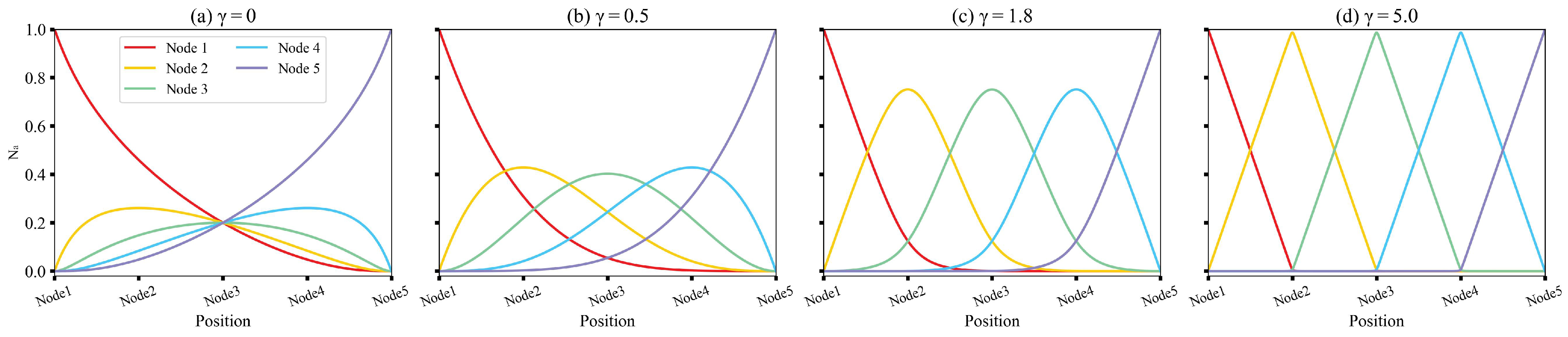
2.1. Local Maximum Entropy Approximation

In this section, we present a brief review of the construction of Local Maximum-Entropy approximation scheme. LME represents a compromise between shape function locality [46] and global entropy [47] in the sense of Pareto optimality. Elements of the pareto set provide a smooth transition between finite element interpolants and meshfree approximants.

Consider a finite set of N distinct nodes in d dimensions, $X=\{{\mathbf{x}}_a,a=1,\cdots ,N\}$, with nodal coordinates ${\mathbf{x}}_a\in {\mathbb{R}}^d$. The domain bounded by the convex hull of X is denoted as $\Omega \subset {\mathbb{R}}^d$. Shape functions of a fixed point $\mathbf{x}$ over the convex domain $\Omega$ are defined for every node ${\mathbf{x}}_a$ as the solution of a convex constrained optimization problem:

$$\begin{array}{cc}\hfill \left(\mathrm{LME}\right)\mathrm{For}\mathrm{fixed}\mathbf{x}\in \Omega ,\mathrm{minimize}& f_{\beta }(\mathbf{x},\mathbf{N})\equiv \beta \sum _{a=1}^n{N}_a\left|\right|\mathbf{x}-{\mathbf{x}}_{\mathbf{a}}{\left|\right|}^2+\sum _{a=1}^n{N}_{a}log{N}_a,\hfill \\ \hfill \mathrm{subject}\mathrm{to}& N_a\left(\mathbf{x}\right)\ge 0,a=1,\dots ,N,\hfill \\ \hfill & \sum N_a\left(\mathbf{x}\right)=1,\hfill \\ \hfill & \sum N_a\left(\mathbf{x}\right){\mathbf{x}}_a=\mathbf{x},\hfill \end{array}$$

(1)

where $\mathbf{N}={(N_1,\cdots ,N_N)}^T$ is the vector of shape functions, and $\beta \in (0,+\infty )$ is Pareto optimal, which takes global max-ent ($\beta \to 0$) and local delaunay ($\beta \to \infty$) schemes as limiting cases. The zeroth- and first-order consistency guarantees the reproduction of affine functions by the approximation scheme and the three mathematical constraints together ensure that the solutions are non-negative and consistent under h-refinement. It is noteworthy that the local max-ent approximation can be extended to higher orders of consistency [36], but they are not covered here due to their increasingly intricate formulation.

It is proved in [37] that LME has a unique solution if and only if $\mathbf{x}\in \Omega$. In principle, the problem is solved by the conventional Lagrange multipliers method as below.

By using shifted nodal coordinates ${\mathbf{y}}_a={\mathbf{x}}_a-\mathbf{x}$ and using the zeroth-order consistency constraint, it is possible to rewrite the first-order consistency condition as

$$\sum _{a=1}^N{N}_a({\mathbf{x}}_a-\mathbf{x})\equiv \sum _{a=1}^N{N}_a{\mathbf{y}}_a=0.$$

(2)

This choice is more efficient and stable in numerical computations than the conditions appear in LME. By introducing the Lagrange multipliers $\mathit{\lambda }\in {\mathbb{R}}^d$ and $\mu \in \mathbb{R}$, the Lagrangian $\mathcal{L}:{\mathbb{R}}^N\times \mathbb{R}\times {\mathbb{R}}^d\mapsto \mathbb{R}$ takes the form:

$$\mathcal{L}(\mathbf{N},\mu ,\mathit{\lambda })=f_{\beta }\left(\mathbf{N}\right)+\mu (\sum _{a=1}^N{N}_a\left(\mathbf{x}\right)-1)+\mathit{\lambda }·\sum _{a=1}^N{N}_a{\mathbf{y}}_a,$$

(3)

where the fixed variable $\mathbf{x}$ is omitted in cost function $f_{\beta }\left(\mathbf{N}\right)$ for notional simplicity. Now the Lagrange multipliers are ready to be determined by standard duality analysis, which also provide a practical way for the calculation of shape functions.

It is convenient to verify that LME satisfies Slater’s condition, in which case strong duality holds. By the KKT (Karush-Kuhn-Tucker) conditions, there exist Lagrange multipliers ${\mathit{\lambda }}^{\ast }$ and ${\mu }^{\ast }$ such that $\{{\mathbf{N}}^{\ast },{\mu }^{\ast },{\mathit{\lambda }}^{\ast }\}$ is a saddle point of the Lagrangian $\mathcal{L}$:

$$\frac{\partial \mathcal{L}}{\partial N_a}({\mathbf{N}}^{\ast },{\mu }^{\ast },{\mathit{\lambda }}^{\ast })=0,$$

(4)

$$\sum N_a^{\ast }\left(\mathbf{x}\right)=1,$$

(5)

$$\sum N_a^{\ast }\left(\mathbf{x}\right){\mathbf{x}}_a=\mathbf{x},$$

(6)

for $\mathbf{x}\in \mathrm{relint}(\Omega )$, where ${\mathbf{N}}^{\ast }$ is the solution to the original problem. From Equation (3), together with conditions (5) and (6), the explicit expression for Equation (4) can be written as

$$\beta \left|\right|\mathbf{x}-{\mathbf{x}}_a{\left|\right|}^2+log{N}_a^{\ast }+1+{\mu }^{\ast }+{\mathit{\lambda }}^{\ast }·({\mathbf{x}}_a-\mathbf{x})=0a=1,\dots ,N,$$

(7)

whence we obtain the solution of (LME) as

$$N_a^{\ast }\left(\mathbf{x}\right)=\frac{Z_a(\mathbf{x},{\mathit{\lambda }}^{\ast })}{exp({\mu }^{\ast }+1)},$$

(8)

where

$$Z_a(\mathbf{x},\mathit{\lambda })=exp[-\beta ||\mathbf{x}-{\mathbf{x}}_a{\left|\right|}^2+\mathit{\lambda }·(\mathbf{x}-{\mathbf{x}}_a)],$$

(9)

and $Z(\mathbf{x},\mathit{\lambda })={\sum }_{a=1}^N{Z}_a(\mathbf{x},\mathit{\lambda })$ is known as the partition function in statistical mechanics.

The Lagrange dual function of the primal problem (1) is given by

$$g(\mu ,\mathit{\lambda })=\underset{N_a\in {\mathbb{R}}^{+}}{inf}\mathcal{L}(\mathbf{N},\mu ,\mathit{\lambda })=-\mu -exp(-\mu -1)Z(\mathbf{x},\mathit{\lambda }),$$

(10)

and the dual problem is

$$\underset{\mu \in \mathbb{R},\mathit{\lambda }\in {\mathbb{R}}^d}{max}g(\mu ,\mathit{\lambda }),$$

(11)

whose solutions are the above optimal Lagrange parameters ${\mathit{\lambda }}^{\ast }$ and ${\mu }^{\ast }$. We can simplify the dual function by maximizing over the dual variable $\mu$ analytically. For fixed $\mathit{\lambda }$, the objective function is maximized when the derivative with respect to $\mu$ equals zero, which gives

$${\mu }^{\ast }+1=logZ(\mathbf{x},\mathit{\lambda }).$$

(12)

Substituting this optimal value of ${\mu }^{\ast }$ back into the dual problem gives the reduced form

$$\underset{\mathit{\lambda }\in {\mathbb{R}}^d}{min}logZ(\mathbf{x},\mathit{\lambda }),$$

(13)

which is an unconstrained geometric program (in a convex form) finally to be solved. The function $F\left(\mathit{\lambda }\right)\equiv logZ(\mathbf{x},\mathit{\lambda })$ for fixed $\mathbf{x}$ is also introduced as a potential function for determining the Lagrange parameter $\mathit{\lambda }$. In our program, it was solved efficiently and robustly by a combination of the Newton-Raphson algorithm and Nelder-Mead simplex algorithm [48].

Note again that the parameter $\beta \in {\mathbb{R}}^{+}$ is used to ponder the locality term against the entropy term in the local maximum entropy approximation. In practice, dimensionless parameter $\gamma$ is used. It is related to $\beta$ by

$$\gamma =\beta h^2,$$

(14)

where h is a local characteristic length of the considered node set X. Hence, the shape functions (8) become

$$N_a\left(\mathbf{x}\right)=\frac{1}{Z(\mathbf{x},{\mathit{\lambda }}^{\ast })}exp\left[-\frac{\gamma }{h^2}\left|\right|\mathbf{x}-{\mathbf{x}}_a{\left|\right|}^2+{\mathit{\lambda }}^{\ast }·(\mathbf{x}-{\mathbf{x}}_a)\right].$$

(15)

Moreover, to obtain a better convergence, the term ${\mathit{\lambda }}^{\ast }·(\mathbf{x}-{\mathbf{x}}_a)$ is scaled depending on the node density. Figure 1 represents LME shape functions for a one-dimensional node set containing five uniformly distributed nodes with different values of $\gamma$. As $\gamma$ tends to 0, the LME scheme transitions into the global max-ent scheme, yielding non-zero shape functions over the entire domain. With an increase in $\gamma$, local influence becomes dominant, making shape functions more compactly supported. At $\gamma =5$, these shape functions are almost identical to the linear interpolation used in Finite Elements. No matter how $\gamma$ changes, the non-negativity of shape functions holds, and the weak Kronecker-delta property at the boundary is consistently satisfied.

It is straightforward to apply this theory to an irregular node set with spatially non-uniform $\gamma$ regardless of the dimension.

The computation of the spatial derivatives of LME shape functions presents challenges, particularly due to the involvement of derivatives of the Lagrange multiplier ${\mathit{\lambda }}^{\ast }\left(\mathbf{x}\right)$. The general computation procedure with non-uniform $\beta \left(\mathbf{x}\right)$ and the explicit form of the derivatives with respect to $\mathbf{x}$ are elucidated in the Appendix A of [37]. They are formulated as

$$\nabla N_a=-N_a{\mathbf{J}}^{\ast -1}·(\mathbf{x}-{\mathbf{x}}_a)+N_a{K}_a\nabla \beta ,$$

(16)

where

$$K_a=\left[\sum _b{N}_b{\parallel \mathbf{x}-{\mathbf{x}}_b\parallel }^2(\mathbf{x}-{\mathbf{x}}_b)\right]·{\mathbf{J}}^{\ast -1}·(\mathbf{x}-{\mathbf{x}}_a)-{\parallel \mathbf{x}-{\mathbf{x}}_a\parallel }^2+U(\mathbf{x},\mathbf{N}),$$

(17)

$${\mathbf{J}}^{\ast }\equiv {\partial }_{\mathit{\lambda }}{\partial }_{\mathit{\lambda }}logZ(\mathbf{x},{\mathit{\lambda }}^{\ast }),$$

(18)

$$U(\mathbf{x},\mathbf{N})\equiv \sum _b{N}_b{\parallel \mathbf{x}-{\mathbf{x}}_b\parallel }^2.$$

(19)

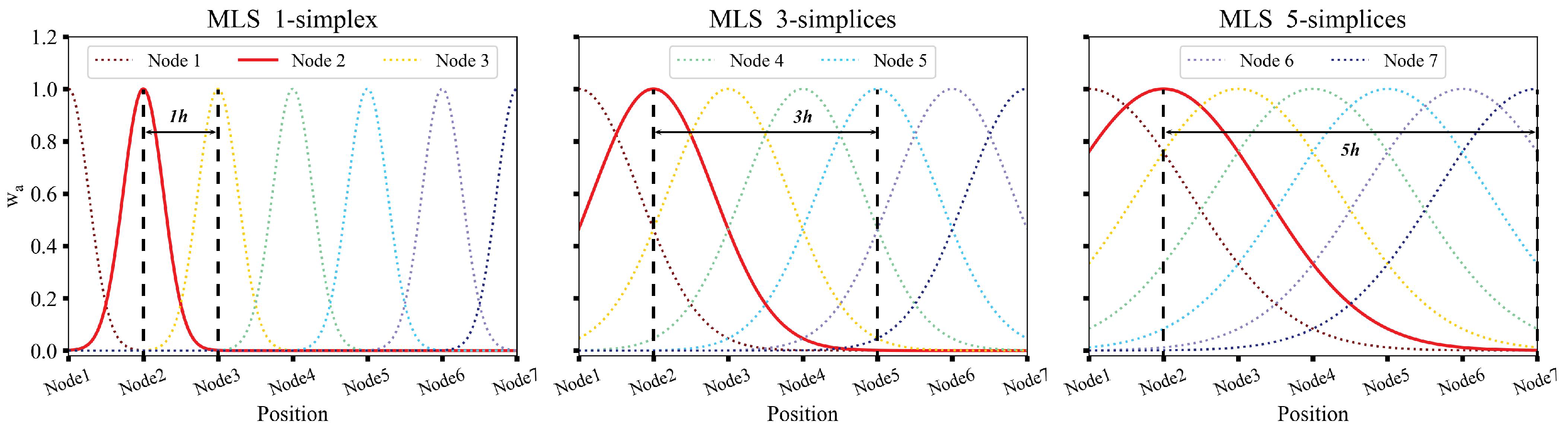
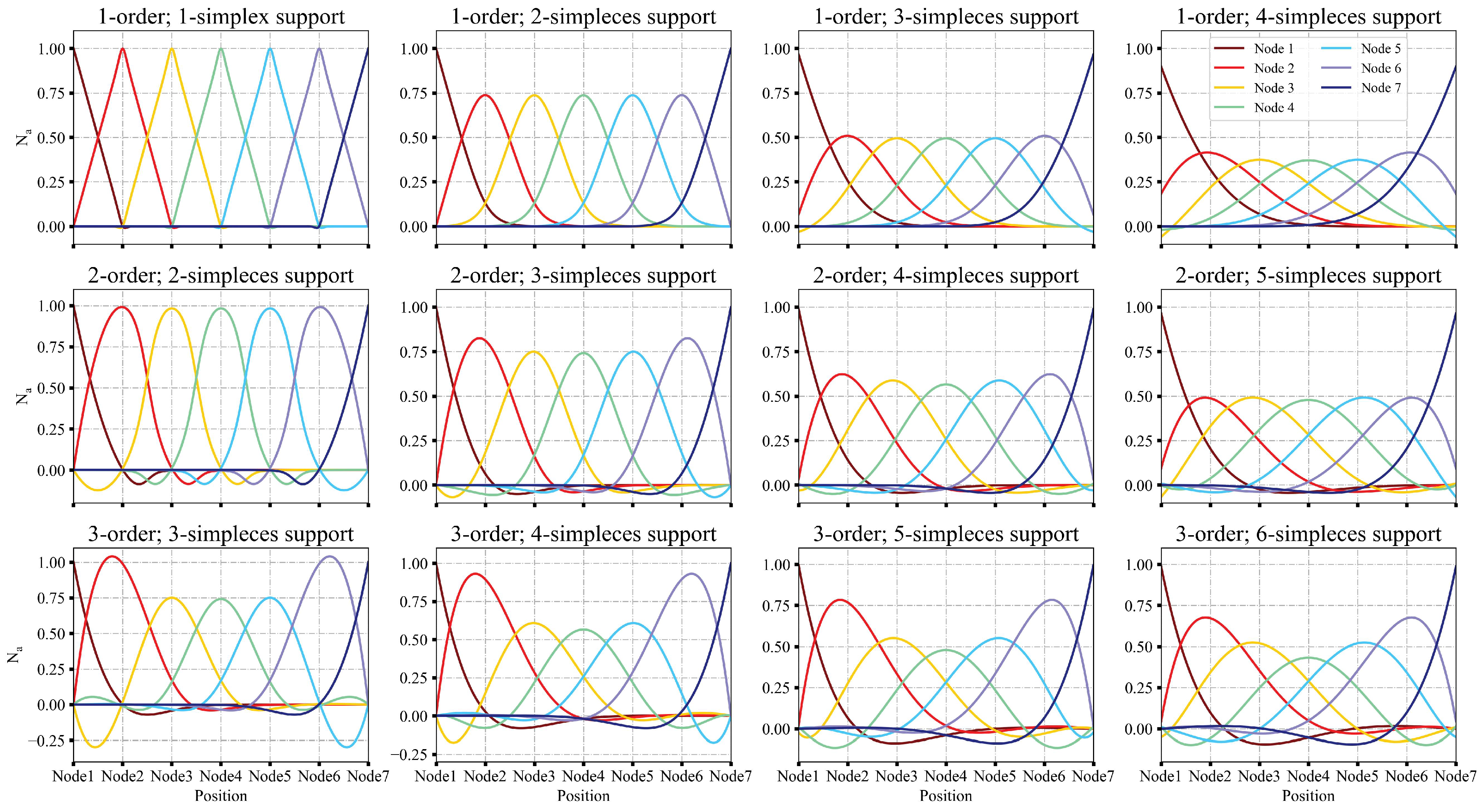
2.2. Moving Least Squares Approximation

In this section, MLS shape functions are constructed for computing an approximation function $u^h\left(\mathbf{x}\right)$ of the real solution $u\left(\mathbf{x}\right)$, while knowing the actual value $u_a\equiv u\left({\mathbf{x}}_a\right)$ at the nodes ${\mathbf{x}}_a$. To do so, a local standard least squares is conducted at the computing point $\overline{\mathbf{x}}$ based on minimizing the sum of the squares of the residuals ${[u_L^h({\mathbf{x}}_a,\overline{\mathbf{x}})-u_a]}^2$ obtained from each node a. While the computing point dynamically moves, the local approximation expression $u_L^h({\mathbf{x}}_a,\overline{\mathbf{x}})$ undergoes modifications, leading to oscillations in the curve.

Subsequently, the idea of compact support domain is being considered. This is performed by the use of a predefined weight function $w_a\left(\mathbf{x}\right)\equiv w(\mathbf{x}-{\mathbf{x}}_a)$ combined with a parameter support radius ${\rho }_a$ for each node a. The most basic one is a constant weight function taking 1 within the support domain and 0 outside. While it meets the essential criterion for a weight function to be non-negative and exhibit a monotonically decreasing behavior as the distance $∥\mathbf{x}-{\mathbf{x}}_a∥$ increases, it may not be the optimal choice since it fails to reflect the greater significance of contributions from closer nodes. From this perspective, the Gaussian weight function and the cubic spline weight function are the most practical choices, with the latter being more efficient due to the lower computational cost compared to the former, which involves the calculation of an exponential.

The Gaussian weight function, as manifested in LME, has been selected as the weight function for MLS. Similar to the partition function in Equation (15), the Gaussian weight function used in MLS is defined as

$$w_a\left(\mathbf{x}\right)=exp\left[-\frac{{\gamma }_a}{h_a^2}{\parallel \mathbf{x}-{\mathbf{x}}_a\parallel }^2\right],$$

(20)

where ${\gamma }_a$ and $h_a$ have same meanings as in Equation (14) but are limited to node a. The support domain is directly determined by ${\rho }_a$, starting from the node and truncated at the periphery of the Gaussian weight function, measured by a parameter tol as

$${\rho }_a=\sqrt{\frac{-logtol}{\gamma }}h,$$

(21)

from which $\gamma$ can be deduced if the size of the support domain is given.

The concept of simplex is used to stand for the radius of the support domain. As depicted in Figure 2, the 1-simplex, 3-simplices, and 5-simplices support domains correspond to values of ${\rho }_a$ being h, $3h$, and $5h$, and so forth. Generally, the value of tol is often chosen as ${10}^{-3}$, in which case $\gamma$ would become 6.9, 0.77 and 0.28 for 1-simplex, 3-simplices, and 5-simplices.

Let $\overline{\Omega }\left(\overline{\mathbf{x}}\right)$ be the intersection of support domains of nodes whose weight function are nonzero at $\overline{\mathbf{x}}$. Record these nodes which have overlapping influences on $\overline{\mathbf{x}}$ and label them from 1 to N. Therefore, the weighted least squares functional, also named as the cost function, at a material point $\overline{\mathbf{x}}$, can be written as

$$\begin{array}{cc}\hfill J& =\frac{1}{2}\sum _{a=1}^N{w}_a\left(\overline{\mathbf{x}}\right){\left[u_L^h({\mathbf{x}}_a,\overline{\mathbf{x}})-u_a\right]}^2\hfill \\ & =\frac{1}{2}\sum _{a=1}^N{w}_a\left(\overline{\mathbf{x}}\right){\left[{\mathbf{p}}^T\left({\mathbf{x}}_a\right)\mathbf{g}\left(\overline{\mathbf{x}}\right)-u_a\right]}^2.\hfill \end{array}$$

(22)

As seen in the above equation, $u_L^h(\mathbf{x},\overline{\mathbf{x}})$ has been resolved into the dot product of a basis function vector $\mathbf{p}\left(\mathbf{x}\right)$ and a coefficient vector $\mathbf{g}\left(\overline{\mathbf{x}}\right)$ as

$$\begin{array}{cc}\hfill u_L^h(\mathbf{x},\overline{\mathbf{x}})& =g_1\left(\overline{\mathbf{x}}\right)p_1\left(\mathbf{x}\right)+g_2\left(\overline{\mathbf{x}}\right)p_2\left(\mathbf{x}\right)+\cdots +g_k\left(\overline{\mathbf{x}}\right)p_k\left(\mathbf{x}\right)\hfill \\ & =\sum _{i=1}^k{g}_i\left(\overline{\mathbf{x}}\right)p_i\left(\mathbf{x}\right)={\mathbf{p}}^T\left(\mathbf{x}\right)\mathbf{g}\left(\overline{\mathbf{x}}\right).\hfill \end{array}$$

(23)

Note that $\mathbf{p}$ can be any basis functions conserving the properties of independence, including polynomial and trigonometric functions. Generally, it would be set as a complete polynomial of order m here out of simpleness. For instance, if $m=3$, $\mathbf{p}$ is a cubic polynomial in 1D such that $\mathbf{p}={\left[1x{x}^2{x}^3\right]}^T$. For the same order in 2D, $\mathbf{p}={\left[1xy{x}^{2}xy{y}^2{x}^3{x}^{2}yx{y}^2{y}^3\right]}^{ T}$. And for $m=2$ in 3D, $\mathbf{p}={\left[1xyz{x}^{2}xyxz{y}^{2}yz{z}^2\right]}^{ T}$. Let k be the number of terms in a complete polynomial basis. It depends on the order m and the dimension, and it can be calculated by the expression listed in

Table 1. Calculation of the number of terms in a complete polynomial basis of order m.

Dimension	k
1D	$m+1$
2D	$(m+1)(m+2)/2$
3D	$(m+1)(m+2)(m+3)/6$

.

$\mathbf{g}\left(\overline{\mathbf{x}}\right)$ signifies that these coefficients are varying with $\overline{\mathbf{x}}$ and the curve is fitted within the local context. These coefficients are obtained by solving Equation (22).

The functional J can also be written in matrix form as

$$J=\frac{1}{2}{\left(\mathbf{P}\mathbf{g}-\mathbf{u}\right)}^T\mathbf{W}\left(\mathbf{P}\mathbf{g}-\mathbf{u}\right),$$

(24)

where $\mathbf{u}$ is a vector of nodal values

$$\mathbf{u}={\left[\begin{array}{cccc}{u}_1& u_2& \cdots & u_N\end{array}\right]}^T,$$

(25)

$\mathbf{P}$ is formed by ${\mathbf{p}}^T\left({\mathbf{x}}_a\right)$ as rows

$$\mathbf{P}={\left[\begin{array}{cccc}{p}_1\left({\mathbf{x}}_1\right)& p_2\left({\mathbf{x}}_1\right)& \cdots & p_k\left({\mathbf{x}}_1\right)\\ ⋮& \ddots & & ⋮\\ ⋮& & \ddots & ⋮\\ p_1\left({\mathbf{x}}_N\right)& p_2\left({\mathbf{x}}_N\right)& \cdots & p_k\left({\mathbf{x}}_N\right)\end{array}\right]}_{N\times k},$$

(26)

and $\mathbf{W}$ is a diagonal N by N matrix such that

$$\mathbf{W}={\left[\begin{array}{cccc}{w}_1\left(\mathbf{x}\right)& & & 0\\ & w_2\left(\mathbf{x}\right)& & \\ & & \ddots & \\ 0& & & w_N\left(\mathbf{x}\right)\end{array}\right]}_{N\times N}.$$

(27)

To minimize J in (24) with respect to $\mathbf{g}\left(\overline{\mathbf{x}}\right)$, $\partial J/\partial \mathbf{g}=\mathbf{0}$ leads to

$${\mathbf{P}}^T\mathbf{W}\mathbf{P}\mathbf{g}={\mathbf{P}}^T\mathbf{W}\mathbf{u}.$$

(28)

Now, let $\mathbf{A}={\mathbf{P}}^T\mathbf{W}\mathbf{P}$ be the moment matrix and $\mathbf{B}={\mathbf{P}}^T\mathbf{W}$. Note that $\mathbf{A}$ is k by k and $\mathbf{B}$ is k by N. $\mathbf{g}$ can be now solved by

$$\mathbf{g}={\mathbf{A}}^{-1}\mathbf{B}\mathbf{u},$$

(29)

when $\mathbf{A}$ is non-singular. And the local approximation function $u_L^h(\mathbf{x},\overline{\mathbf{x}})$ is then given by:

$$u_L^h(\mathbf{x},\overline{\mathbf{x}})={\mathbf{p}}^T\left(\mathbf{x}\right)\mathbf{g}\left(\overline{\mathbf{x}}\right)={\mathbf{p}}^T\left(\mathbf{x}\right){\mathbf{A}}^{-1}\left(\overline{\mathbf{x}}\right)\mathbf{B}\left(\overline{\mathbf{x}}\right)\mathbf{u}.$$

(30)

Obviously, it is important to discuss how to derive the global MLS approximation function $u^h\left(\mathbf{x}\right)$ from the local approximation function $u_L^h(\mathbf{x},\overline{\mathbf{x}})$. Firstly, an interpolated value $u_L^h(\overline{\mathbf{x}},\overline{\mathbf{x}})$ at $\overline{\mathbf{x}}$ can be obtained from the local approximation, abbreviated as $u_L^h\left(\overline{\mathbf{x}}\right)$. Numerically, the global MLS approximation is composed of the set of all the evaluations of the local approximation at $\mathbf{x}=\overline{\mathbf{x}}$, i.e.,

$$u^h\left(\mathbf{x}\right)={\mathbf{p}}^T\left(\mathbf{x}\right){\mathbf{A}}^{-1}\left(\mathbf{x}\right)\mathbf{B}\left(\mathbf{x}\right)\mathbf{u}.$$

(31)

Rewrite it as a form of shape functions,

$$u^h\left(\mathbf{x}\right)=\mathbf{N}\left(\mathbf{x}\right)\mathbf{u}=\sum _{a=1}^N{N}_a\left(\mathbf{x}\right)u_a,$$

(32)

where $N_a$ is the shape function regarding node ${\mathbf{x}}_a$, and is defined by:

$$N_a\left(\mathbf{x}\right)={\mathbf{p}}^T{\mathbf{A}}^{-1}{\mathbf{B}}_a,$$

(33)

where the subscript a represents the a-th column of matrix $\mathbf{B}$.

Figure 3 shows 1D MLS shape functions for different orders and support sizes. Generally, larger the support domain, the wider the shape functions. When the first-order polynomial basis is used, the shape functions closely resemble those obtained through the LME scheme. But discrepancies arise at two crucial points. Firstly, the non-negativity is broken, as observed in the fourth image with a support domain radius of 4-simplices, where curves dip below zero near the boundary. This issue intensifies with higher-order polynomial bases. Secondly, these shape functions do not satisfy the Kronecker-delta property at the boundaries of ${\Omega }_{MLS}$, especially with an increased support domain radius. This will arouse difficulties in imposing essential boundary conditions. Excellently, MLS is able to achieve shape functions of high continuity and compatibility by choosing low-order polynomial bases with proper weight functions since the approximation would inherit the continuity of the weight function.

Now, an effective way to compute the derivatives proposed by Belytschko [49] is detailed. Let us define ${\mathbf{p}}^T\left(\mathbf{x}\right){\mathbf{A}}^{-1}\left(\mathbf{x}\right)$ as ${\mathit{\alpha }}^T\left(\mathbf{x}\right)$. Since $\mathbf{A}$ is symmetric, this equation can also be written as

$$\mathbf{A}\mathit{\alpha }=\mathbf{p},$$

(34)

where $\mathbf{A}={\mathbf{P}}^T\mathbf{W}\mathbf{P}$ is the moment matrix defined in the previous section and $\mathit{\alpha }$ a k by 1 vector. Therefore, $\mathit{\alpha }$ can be easily determined by inversing $\mathbf{A}$:

$$\mathit{\alpha }={\mathbf{A}}^{-1}\mathbf{p}.$$

(35)

Differentiate (34) with respect to $\mathbf{x}$ (denoted by the subscript “, $\mathbf{x}$”):

$${\mathbf{A}}_{,\mathbf{x}}\mathit{\alpha }+\mathbf{A}{\mathit{\alpha }}_{,\mathbf{x}}={\mathbf{p}}_{,\mathbf{x}}.$$

(36)

Since $\mathit{\alpha }$, $\mathbf{A}$, ${\mathbf{A}}^{-1}$ are known and ${\mathbf{p}}_{,\mathbf{x}}$ can be easily found, ${\mathit{\alpha }}_{,\mathbf{x}}$ is computed as

$${\mathit{\alpha }}_{,\mathbf{x}}={\mathbf{A}}^{-1}\left({\mathbf{p}}_{,\mathbf{x}}-{\mathbf{A}}_{,\mathbf{x}}\mathit{\alpha }\right).$$

(37)

The derivatives of shape functions are then given by

$$N_{a,\mathbf{x}}={\mathit{\alpha }}_{,\mathbf{x}}^T{\mathbf{B}}_a+{\mathit{\alpha }}^T{\mathbf{B}}_{a,\mathbf{x}}.$$

(38)

2.3. Blending Algorithm for MLS

In order to enforce essential boundary conditions through the MLS approximation, Fernandez-Mendez and Huerta [50,51] introduced a blending algorithm, facilitating the coupling of a meshfree approximation with the classic Finite Element (FE) method. This section outlines the procedure for integrating the MLS approximation with FE interpolation.

We are going to build modified MLS shape functions. Let us consider a domain $\Omega ={\Omega }_{FEM}\cup {\Omega }_{MLS}$. ${\Omega }_{FEM}$ and ${\Omega }_{MLS}$ represent areas where the FE basis is complete and MLS shape functions are defined, respectively. The region ${\Omega }_{MIX}$, contained in ${\Omega }_{MLS}$, denotes the layer of elements where the MLS shape functions should be modified to meet the consistency condition due to incomplete FE bases. From now on, ${\widehat{N}}_a$ will denote the modified MLS shape functions and $N_a^{MIX}={\widehat{N}}_a+N_a^{FEM}$ will represent the final shape functions in the mixed domain. Examples of the discretized domain in 1D and 2D, where the coupling of FEM and MLS interpolation is applied, are shown in Figure 4 and Figure 5.

As shown, there are many hybrid nodes which belong to both ${\Omega }_{FEM}$ and ${\Omega }_{MLS}$. Now let us consider a material point $\mathbf{x}$ in the mixed domain. The objective is to ensure that the new shape functions in the mixed domain satisfy the consistency conditions. Here, two considerations are involved: firstly, the FEM shape functions must remain unchanged, and secondly, the MLS shape functions need to be adjusted to uphold consistency. It is crucial to emphasize that the consistency order is determined by the lowest consistency order verified by the FE shape functions and MLS shape functions separately. For example, if the FE shape functions are linear, then the consistency order of the mixed shape functions will be limited to one.

In order to retain the integrity of the FEM shape functions within the mixed domain, the modified MLS shape functions ${\widehat{N}}_a$ must be set to zero at the mixed nodes to satisfy the consistency equations, which at $\mathbf{x}$ are:

$$\sum _a{\widehat{N}}_a\left(\mathbf{x}\right)\mathbf{p}\left({\mathbf{x}}_a\right)+\sum _b{N}_b^{FEM}\left(\mathbf{x}\right)\mathbf{p}\left({\mathbf{x}}_b\right)=\mathbf{p}\left(\mathbf{x}\right),$$

(39)

where $\mathbf{p}$ is the basis function vector.

Introduce an unknown vector $\mathbf{c}\left(\mathbf{x}\right)\equiv {[c_1{c}_2\dots c_k]}^T$ to determine ${\widehat{N}}_a\left(\mathbf{x}\right)$:

$${\widehat{N}}_a\left(\mathbf{x}\right)={\mathbf{c}}^T\left(\mathbf{x}\right)\mathbf{p}\left({\mathbf{x}}_a\right)w_a\left(\mathbf{x}\right),$$

(40)

and Equation (39) thus becomes

$$\mathbf{p}\left(\mathbf{x}\right)=\sum _a{\mathbf{c}}^T\left(\mathbf{x}\right)\mathbf{p}\left({\mathbf{x}}_a\right)w_a\left(\mathbf{x}\right)\mathbf{p}\left({\mathbf{x}}_a\right)+\sum _b{N}_b^{FEM}\left(\mathbf{x}\right)\mathbf{p}\left({\mathbf{x}}_b\right).$$

(41)

Reiterate the definition of the moment matrix $\mathbf{A}={\mathbf{P}}^T\mathbf{W}\mathbf{P}$, resulting in

$$\mathbf{A}\mathbf{c}=\mathbf{p}\left(\mathbf{x}\right)-\sum _b{N}_b^{FEM}\left(\mathbf{x}\right)\mathbf{p}\left({\mathbf{x}}_b\right),$$

(42)

where $\mathbf{c}$ can be solved as

$$\mathbf{c}={\mathbf{A}}^{-1}\left(\mathbf{p}\left(\mathbf{x}\right)-\sum _b{N}_b^{FEM}\left(\mathbf{x}\right)\mathbf{p}\left({\mathbf{x}}_b\right)\right).$$

(43)

Therefore, we can reuse $\mathbf{B}={\mathbf{P}}^T\mathbf{W}$ and rewrite the modified MLS shape functions as following:

$${\widehat{N}}_a\left(\mathbf{x}\right)={\mathbf{A}}^{-1}\left(\mathbf{x}\right)\left(\mathbf{p}\left(\mathbf{x}\right)-\sum _b{N}_b^{FEM}\left(\mathbf{x}\right)\mathbf{p}\left({\mathbf{x}}_b\right)\right){\mathbf{B}}_a\left(\mathbf{x}\right).$$

(44)

Finally, the general shape functions $N_a$ are defined over $\Omega$ as

$$\forall \mathbf{x}\in \Omega ,N_a\left(\mathbf{x}\right)=\left\{\begin{array}{c}{N}_a^{FEM}\left(\mathbf{x}\right)\\ N_a^{FEM}\left(\mathbf{x}\right)+{\widehat{N}}_a\left(\mathbf{x}\right)\\ N_a^{MLS}\left(\mathbf{x}\right)\end{array}\begin{array}{cc}\hfill & \mathrm{if}\mathbf{x}\in {\Omega }_{FEM}\hfill \\ \hfill & \mathrm{if}\mathbf{x}\in {\Omega }_{MIX}\hfill \\ \hfill & \mathrm{if}\mathbf{x}\in {\Omega }_{MLS}\setminus {\Omega }_{MIX}\hfill \end{array}\right.,$$

(45)

and the derivatives can be calculated directly from Equation (45):

$$\forall \mathbf{x}\in \Omega ,N_{a,\mathbf{x}}\left(\mathbf{x}\right)=\left\{\begin{array}{c}{N}_{a,\mathbf{x}}^{FEM}\left(\mathbf{x}\right)\\ N_{a,\mathbf{x}}^{FEM}\left(\mathbf{x}\right)+{\widehat{N}}_{a,\mathbf{x}}\left(\mathbf{x}\right)\\ N_{a,\mathbf{x}}^{MLS}\left(\mathbf{x}\right)\end{array}\begin{array}{cc}\hfill & \mathrm{if}\mathbf{x}\in {\Omega }_{FEM}\hfill \\ \hfill & \mathrm{if}\mathbf{x}\in {\Omega }_{MIX}\hfill \\ \hfill & \mathrm{if}\mathbf{x}\in {\Omega }_{MLS}\setminus {\Omega }_{MIX}\hfill \end{array}\right.,$$

(46)

where the gradient ${\widehat{N}}_{a,\mathbf{x}}$ is obtained by direct derivation of Equation (44):

$$\begin{array}{cc}\hfill {\widehat{N}}_{a,\mathbf{x}}\left(\mathbf{x}\right)=& {\mathbf{A}}_{,\mathbf{x}}^{-1}\left(\mathbf{x}\right)\left(\mathbf{p}\left(\mathbf{x}\right)-\sum _b{N}_b^{FEM}\left(\mathbf{x}\right)\mathbf{p}\left({\mathbf{x}}_b\right)\right){\mathbf{B}}_a\left(\mathbf{x}\right)\hfill \\ & +{\mathbf{A}}^{-1}\left(\mathbf{x}\right)\left({\mathbf{p}}_{,\mathbf{x}}\left(\mathbf{x}\right)-\sum _b{N}_{b,\mathbf{x}}^{FEM}\left(\mathbf{x}\right)\mathbf{p}\left({\mathbf{x}}_b\right)\right){\mathbf{B}}_a\left(\mathbf{x}\right)\hfill \\ \hfill & +{\mathbf{A}}^{-1}\left(\mathbf{x}\right)\left(\mathbf{p}\left(\mathbf{x}\right)-\sum _b{N}_b^{FEM}\left(\mathbf{x}\right)\mathbf{p}\left({\mathbf{x}}_b\right)\right){\mathbf{B}}_{a,\mathbf{x}}\left(\mathbf{x}\right).\hfill \end{array}$$

(47)

Figure 6 shows the mixed shape functions for the one-dimensional case presented in Figure 4.

3. Numerical Examples

This section aims to compare the capabilities of LME and MLS approximants within the framework of OTM, focusing on the accuracy and the convergence rate of the numerical solutions. The OTM method utilizes two sets of points: nodal points and material points. Nodal points, containing position information, describe the deformation of a structure, while material points represent the continuum and carry all physical information. Numerical integration is performed based on material points, akin to the MPM [10,52].

To position the material points, a mesh generated by an arbitrary third-party software is employed. After discretizing the computational domain into a list of elements, the material points are created and distributed at positions such as Gauss points through a loop over all the elements. It is crucial to note that the mesh and elements are only used for material point creation, and once this is accomplished, they are no longer needed or used. Only the nodes and the material points are conserved for subsequent computations.

The original MLS approximation scheme, introduced by Belytschko, lacks the Kronecker-delta property at the boundary, making the imposition of essential boundary conditions less straightforward compared to OTM equipped with the LME scheme. In the subsequent thermal examples, a modified MLS, detailed in Section 2.3, is adopted to enforce prescribed values along the boundaries. The numerical errors introduced by essential boundary conditions may be neglected, allowing us to focus on comparing the shape function performance based on their positivity properties. This modification is implemented exclusively at the interpolation level through the blending algorithm, proving to be an efficient, robust, and versatile technique applicable to various meshfree codes, including OTM or EFG. Unlike the original MLS, the modified version ensures both numerical stability and a uniform order of consistency, leading to convergence across the computational domain.

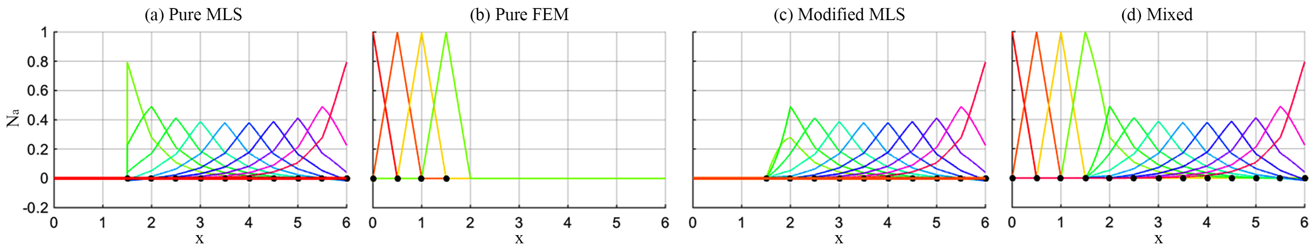
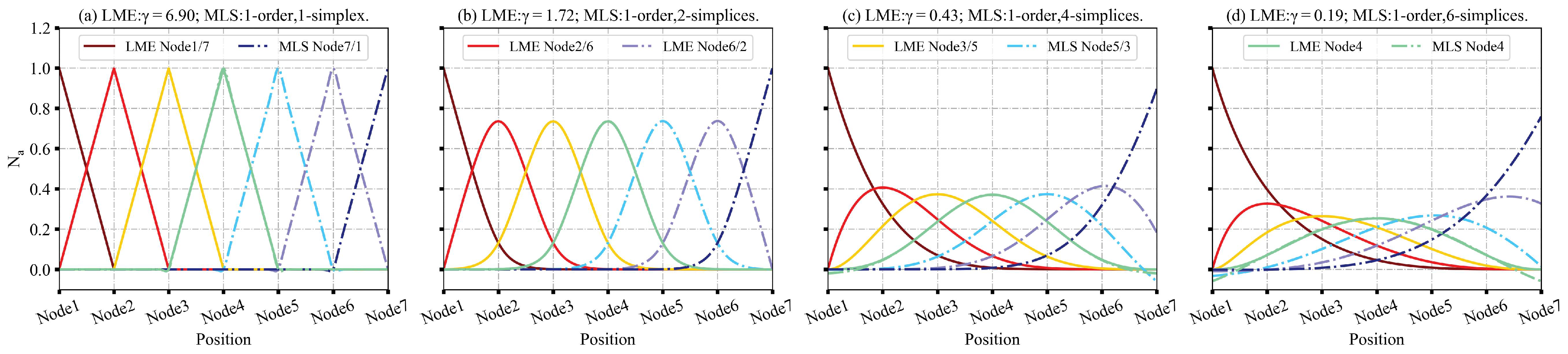
3.1. LME and MLS Shape Functions in 1D

A comparison between the LME and MLS shape functions in one dimension is presented in Figure 7. The dimensionless length has been normalized to the unit and discretized into seven regular nodes. The connection between LME and MLS is established through the dimensionless parameter $\gamma$ used in Equations (15) and (20) based on the Gaussian weight function. Due to the inherent symmetry of the node set, the two types of shape functions are placed in the same image in a comparative scenario, distinguished by different line styles. LME shape functions are drawn in solid lines at Node1 to Node4, while MLS shape functions are drawn in dashdot lines at Node4 to Node7.

As shown in Figure 7a,b, shape functions for LME and the first-order MLS of the same node almost have no difference within a local context, where the radius of the support domain is smaller than 2-simplices. When the support domain expands, MLS shape functions are likely to take negative values away from the nodal center and fail to satisfy the Kronecker-delta property at the boundary of the domain, as illustrated in Figure 7c,d. The presence of negative shape functions may induce unphysical deformations or responses in the engineering applications, given that physical quantities like temperatures and currents inherently cannot be negative. This can lead to inaccuracies in the predictions of the analysis and make it difficult for iterative solvers to converge.

Moreover, in the case of a small radius ${\rho }_a$, the utilization of high-order polynomial bases in MLS renders the least squares minimization problem ill-posed due to an insufficient number of nodes within the support domain. The usual solution requires the expansion of the influence domain for each material point to eliminate the singularity of the moment matrix $\mathbf{A}$. Additionally, Joldes [53] proposed a robust modified MLS method that maintains the support domain size while addressing the singularity issue by augmenting the error functional (24) with additional constraints.

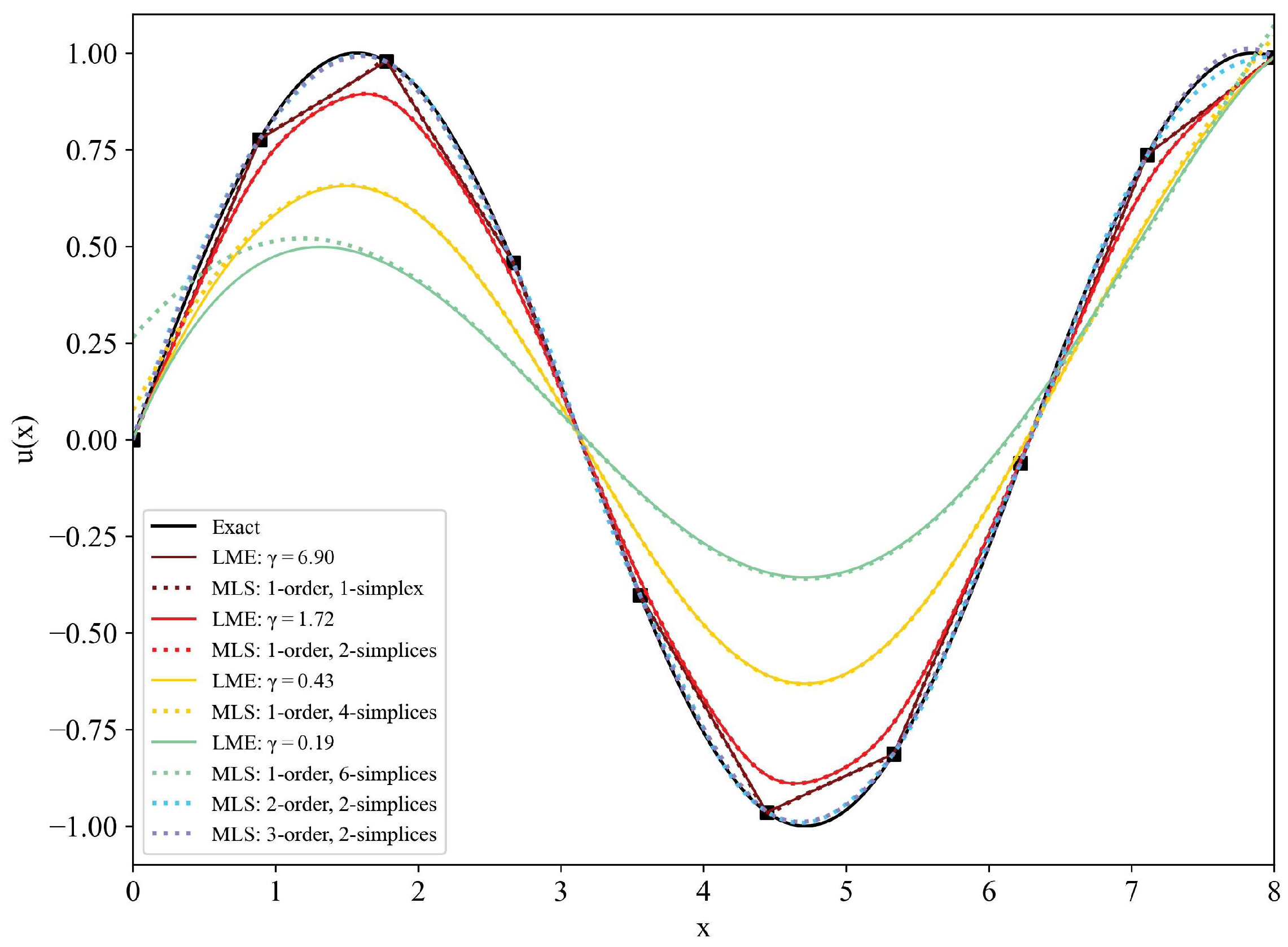
3.2. Approximation of Sine Function in 1D

By using a uniform distribution of 10 nodes within $[0,8]$, the approximations of a non-polynomial function $u\left(x\right)=sinx$ under LME and MLS for different values of $\gamma$ and ${\rho }_a$ are shown in Figure 8. The approximation accuracy is determined by the $L_2$-norm:

$${\parallel e^h\parallel }_2^2={\parallel u-u^h\parallel }_2^2={\int }_0^8{\left(u\left(x\right)-u^h\left(x\right)\right)}^{2}dx,$$

(48)

where $e^h$ represents the error between the approximated value $u^h$ and the exact value u. The definite integral is estimated by the trapezoid rule of 2000 sub-intervals for numerical integration.

The outcomes are depicted in Figure 8 and quantified in

Table 2. Error of approximations of the sine function for LME and MLS under different conditions.

Approximation	${\parallel \mathit{u}-{\mathit{u}}^{\mathit{h}}\parallel }_2^2$	Approximation	${\parallel \mathit{u}-{\mathit{u}}^{\mathit{h}}\parallel }_2^2$
MLS: 1-order, ${\rho }_a=$ 1-simplex	0.0203	LME: $\gamma =6.90$	0.0205
MLS: 1-order, ${\rho }_a=$ 2-simplices	0.0448	LME: $\gamma =1.72$	0.0451
MLS: 1-order, ${\rho }_a=$ 3-simplices	0.1742	LME: $\gamma =0.77$	0.1744
MLS: 1-order, ${\rho }_a=$ 4-simplices	0.4094	LME: $\gamma =0.43$	0.4171
MLS: 1-order, ${\rho }_a=$ 5-simplices	0.7210	LME: $\gamma =0.28$	0.7226
MLS: 1-order, ${\rho }_a=$ 6-simplices	1.0615	LME: $\gamma =0.19$	1.0918
MLS: 2-order, ${\rho }_a=$ 2-simplices	0.0015
MLS: 3-order, ${\rho }_a=$ 2-simplices	0.0006

. The findings reveal that the approximation accuracy of LME closely aligns with that of the classical first-order MLS when they share similar support domain sizes. Notably, the approximation error diminishes with a reduction in the support domain size. As the support domain size contracts to 1-simplex, both approximations coincide with the linear interpolation used in finite elements. The failure of MLS to satisfy the Kronecker-delta property is confirmed at $x=0$ and $x=8$, as observed in the yellow and green dashed lines.

Furthermore, Figure 8 clearly shows the advantage of using higher-order polynomial basis functions. The higher-order MLS has better approximation properties, leading to better solution accuracy as compared to the first-order MLS and LME, albeit at the expense of increased computational effort.

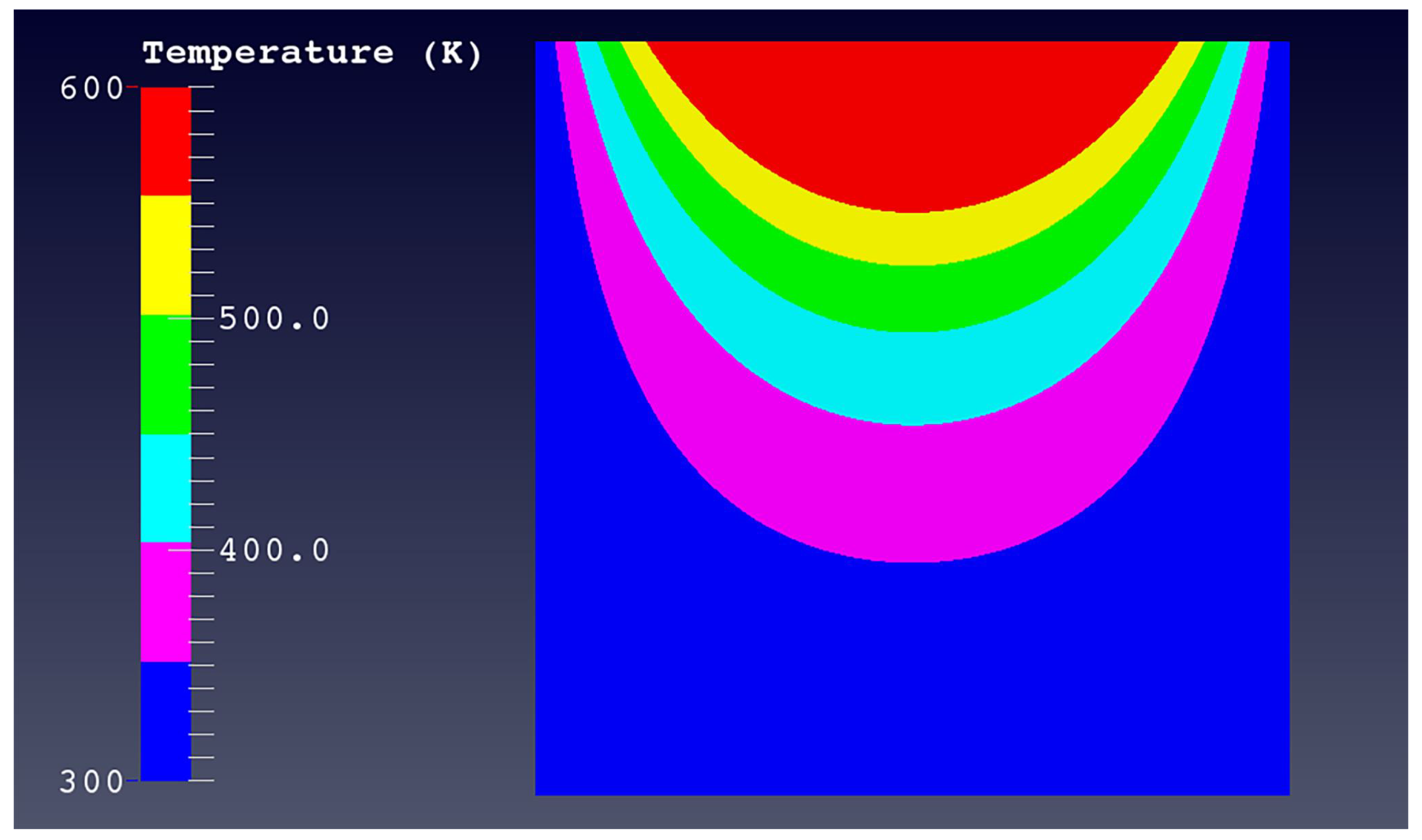
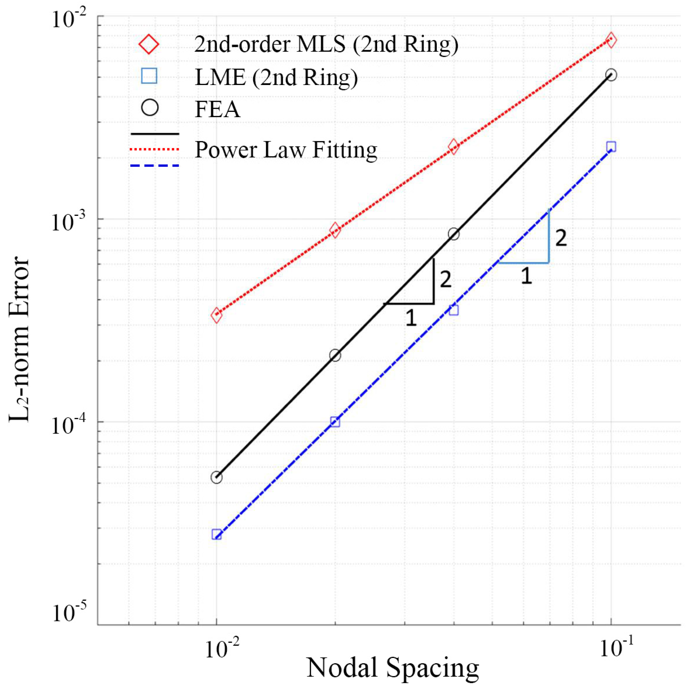
3.3. Thermal Problem with Dirichlet Boundary Conditions

In the following two examples, the modified MLS is utilized to impose essential boundary conditions. Once the influence of boundary conditions on the performance of approximation schemes is eliminated, the focus will shift to highlighting the effectiveness of non-negative shape functions.

Here, we consider thermal conduction through a plate whose size is 1 by 1. This Laplace problem is described in the mathematical form (49):

$$\Delta u=0\mathrm{in}\Omega ={[0,1]}^2,$$

(49a)

$$u(0,y)=u(1,y)=u(x,0)=300,$$

(49b)

$$u(x,1)=x(1-x)\ast 2000+300,$$

(49c)

of which the exact solution is given by

$$u(x,y)=\frac{4}{{\pi }^3}\sum _{i=0}^{\infty }\frac{1-{(-1)}^i}{i^{3}sinh\left(i\pi \right)}sin\left(i\pi x\right)sinh\left(i\pi y\right)\ast 2000+300.$$

(50)

A representative of the initial mesh of regular nodes is shown in Figure 9, where the neighborhood of each material point is composed of all the nodes within the second ring around it. The result obtained from the LME approximation is given by Figure 10. The LME approximants satisfy a weak Kronecker-delta property at the boundary of the convex hull of the nodes, which facilitates the imposition of essential boundary conditions. In the case of the MLS approximants, the blending algorithm described in the Section 2.3 is used for proper imposition of essential boundary conditions.

Figure 11 compares the computed solutions using different approximation schemes with the analytical solution (50) by the $L_2$-norm. The total number of nodes, which are used to fit the convergence rate, varies from 100 to 10,000 in maximum. It shows that both Finite Element Analysis (FEA) and LME analysis have a convergence order of 2 whereas the modified MLS approximation has a smaller convergence order and accuracy.

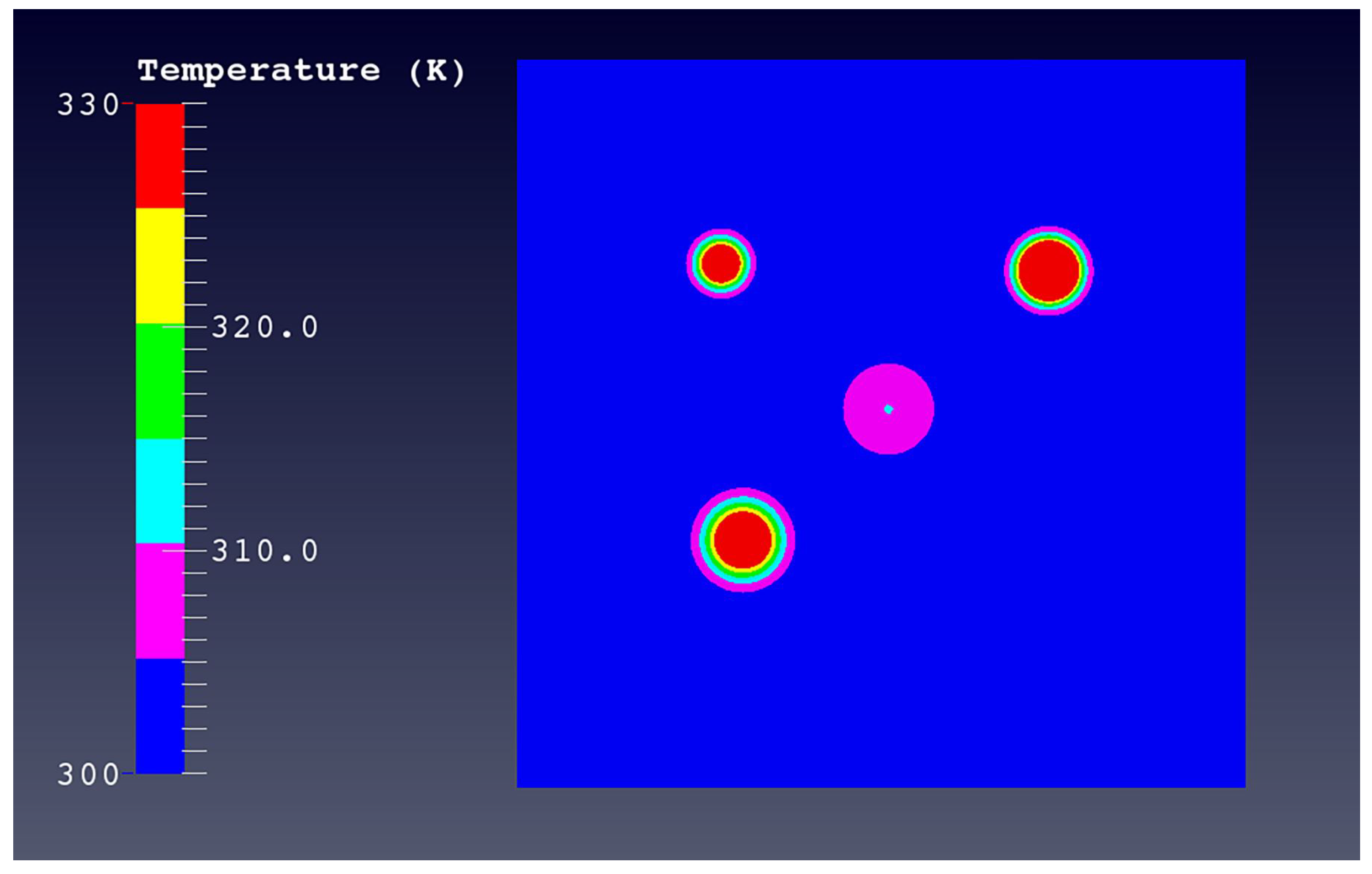
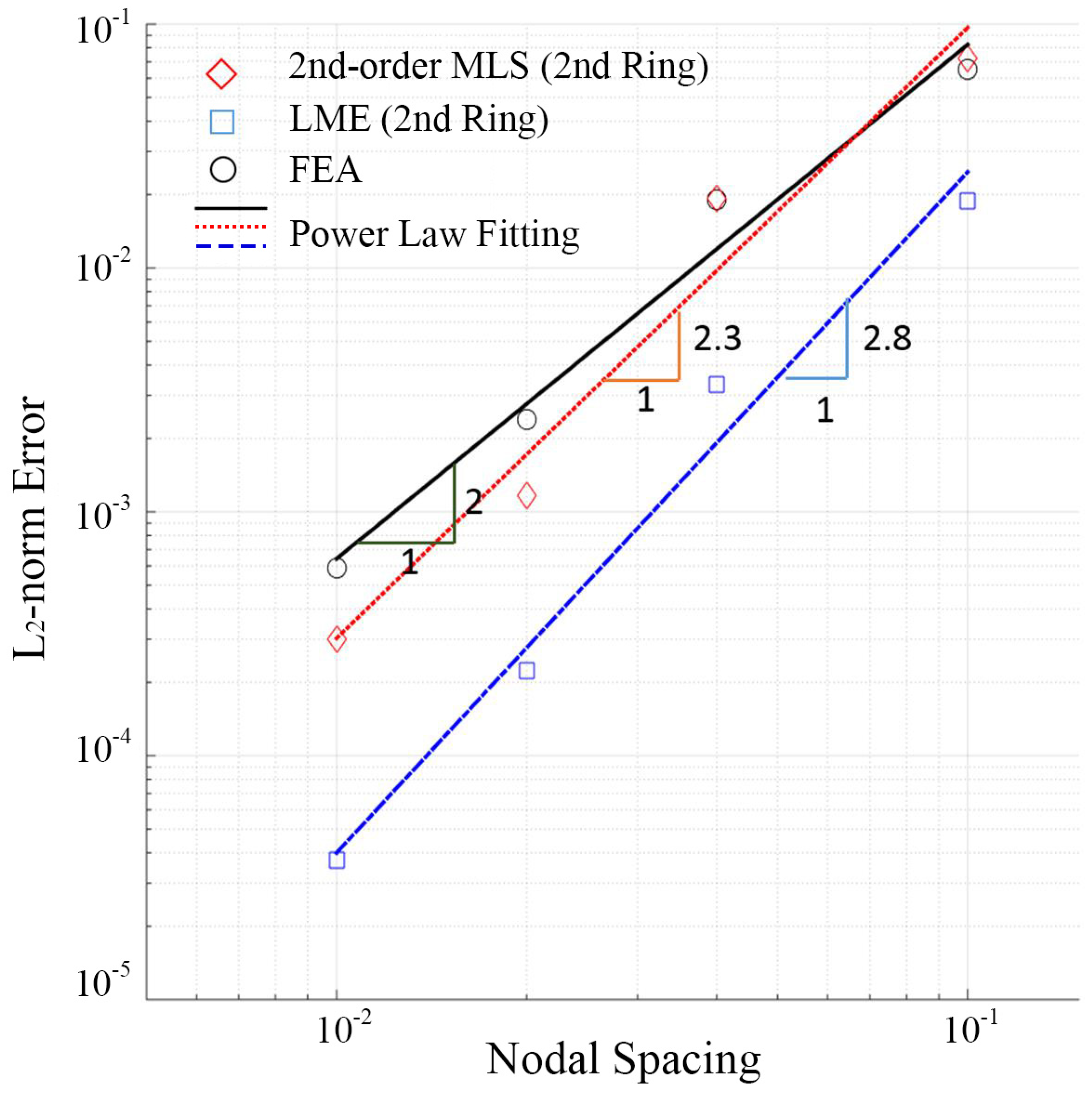
3.4. Thermal Problem with Heat Sources

This example further validates the significance of the non-negativity of shape functions. In this numerical case, localised heat sources are considered in a heat conduction problem and we present the convergence in $L_2$-norm of the FE interpolants, LME approximants and MLS approximants in the Galerkin solution of the Poisson boundary-value problem defined by

$$-\Delta u=s(x,y)\mathrm{in}\Omega ={[0,1]}^2,$$

(51a)

$$u=\overline{u}\mathrm{on}\partial \Omega ,$$

(51b)

where the exact solution of this problem is given by

$$u(x,y)=\sum _{i=1}^4{A}_i{e}^{-\beta \left[{(x-x_i)}^2+{(y-y_i)}^2\right]}.$$

(52)

The coefficients that appear in the exact solution are provided in

Table 3. Coefficients to calculate the exact solution to the Poisson problem.

i	${\mathit{A}}_{\mathit{i}}$	${\mathit{\beta }}_{\mathit{i}}$	${\mathit{x}}_{\mathit{i}}$	${\mathit{y}}_{\mathit{i}}$
1	10	180	$0.51$	$0.52$
2	50	450	$0.31$	$0.34$
3	100	800	$0.73$	$0.71$
4	50	1000	$0.28$	$0.72$

.

The mesh used in this example is same as that illustrated in Figure 9. The equilibrium state obtained from the simulation using the LME approximation is shown in Figure 12.

The total number of nodes to fit the convergence rate varies from 100 to 10,000. As seen in Figure 13, the LME approximation gives both the best accuracy and convergence rate but it is worth noticing that the MLS approximation gives better results in this example than FEA.

As observed in the preceding two examples, the accuracy of the solution is closely linked to the characteristics of the shape functions in numerous numerical methods. Positive shape functions are more likely to be compatible with certain physical fields. Specifically, in the realm of heat conduction analysis, the incorporation of positive temperature shape functions ensures that the physical constraints are satisfied and makes the numerical solution more physically meaningful.

4. Conclusions

This paper presents a thorough examination of two prominent approximation techniques, specifically, the Local Maximum-Entropy and Moving Least Squares methods, within the context of Optimal Transportation Meshfree, a Galerkin-based meshfree approach. Four numerical experiments were undertaken to elucidate the comparisons and interrelations between these schemes. These experiments involved an analysis of their shape function characteristics, assessing their capabilities in approximating non-polynomial functions and performance in numerical simulations.

Our studies highlight the significance of maintaining the positivity of shape functions and their weak Kronecker-delta property at the boundary for ensuring the stability, accuracy, and physical interpretability of numerical solutions across diverse applications. It facilitates a convenient implementation of the essential boundary conditions commonly encountered in thermal-mechanical problems. Furthermore, when solving heat transfer equations using the OTM method, we observed that the accuracy and convergence rate are superior when employing the LME shape functions compared to MLS approximation.

Our results indicate that the classical LME performs comparably to first-order MLS using the Gaussian weight function in a regular node set. However, as the consistency order is raised, both methods demonstrate enhanced accuracy. The straightforward extension of MLS to higher orders makes it a preferred option when striving for highly accurate results. However, in the case of irregular nodal distribution, modifications [53,54,55] to MLS become necessary to enable the use of high-order basis functions without expanding the support domain.

In general, when conducting a comparative analysis of the Local Maximum-Entropy and Moving Least Squares approximation schemes, it becomes evident that both methods exhibit significant utility within the OTM framework for solving engineering problems. The selection between these approaches may hinge on factors such as computational efficiency and the type of differential equations. Consequently, it is crucial to meticulously assess the distinctive attributes of the data and the underlying nature of the problem before making a decision.

References

1. Belytschko, T.; Krongauz, Y.; Organ, D.; Fleming, M.; Krysl, P. Meshless methods: An overview and recent developments. Comput. Methods Appl. Mech. Eng. 1996, 139, 3–47. [Google Scholar] [CrossRef]
2. Liu, G. An overview on meshfree methods: For computational solid mechanics. Int. J. Comput. Methods 2016, 13, 1630001. [Google Scholar] [CrossRef]
3. Chen, J.S.; Hillman, M.; Chi, S.W. Meshfree methods: Progress made after 20 years. J. Eng. Mech. 2017, 143, 04017001. [Google Scholar] [CrossRef]
4. Lucy, L.B. A numerical approach to the testing of the fission hypothesis. Astron. J. 1977, 82, 1013–1024. [Google Scholar] [CrossRef]
5. Gingold, R.A.; Monaghan, J.J. Smoothed particle hydrodynamics: Theory and application to non-spherical stars. Mon. Not. R. Astron. Soc. 1977, 181, 375–389. [Google Scholar] [CrossRef]
6. Liu, G.R.; Liu, M.B. Smoothed Particle Hydrodynamics: A Meshfree Particle Method; World Scientific: Singapore, 2003. [Google Scholar]
7. Belytschko, T.; Lu, Y.Y.; Gu, L. Element-free Galerkin methods. Int. J. Numer. Methods Eng. 1994, 37, 229–256. [Google Scholar] [CrossRef]
8. Dolbow, J.; Belytschko, T. An introduction to programming the meshless Element F reeGalerkin method. Arch. Comput. Methods Eng. 1998, 5, 207–241. [Google Scholar] [CrossRef]
9. Liu, W.K.; Jun, S.; Zhang, Y.F. Reproducing kernel particle methods. Int. J. Numer. Methods Fluids 1995, 20, 1081–1106. [Google Scholar] [CrossRef]
10. Sulsky, D.; Chen, Z.; Schreyer, H.L. A particle method for history-dependent materials. Comput. Methods Appl. Mech. Eng. 1994, 118, 179–196. [Google Scholar] [CrossRef]
11. Zhang, X.; Chen, Z.; Liu, Y. The Material Point Method: A Continuum-Based Particle Method for Extreme Loading Cases; Academic Press: Cambridge, MA, USA, 2016. [Google Scholar]
12. Braun, J.; Sambridge, M. A numerical method for solving partial differential equations on highly irregular evolving grids. Nature 1995, 376, 655–660. [Google Scholar] [CrossRef]
13. Sukumar, N.; Moran, B.; Belytschko, T. The natural element method in solid mechanics. Int. J. Numer. Methods Eng. 1998, 43, 839–887. [Google Scholar] [CrossRef]
14. Sukumar, N.; Moran, B.; Yu Semenov, A.; Belikov, V. Natural neighbour Galerkin methods. Int. J. Numer. Methods Eng. 2001, 50, 1–27. [Google Scholar] [CrossRef]
15. Li, B.; Habbal, F.; Ortiz, M. Optimal transportation meshfree approximation schemes for fluid and plastic flows. Int. J. Numer. Methods Eng. 2010, 83, 1541–1579. [Google Scholar] [CrossRef]
16. Wang, H.; Liao, H.; Fan, Z.; Fan, J.; Stainier, L.; Li, X.; Li, B. The Hot Optimal Transportation Meshfree (HOTM) method for materials under extreme dynamic thermomechanical conditions. Comput. Methods Appl. Mech. Eng. 2020, 364, 112958. [Google Scholar] [CrossRef]
17. Johnson, G.R.; Beissel, S.R. Normalized smoothing functions for SPH impact computations. Int. J. Numer. Methods Eng. 1996, 39, 2725–2741. [Google Scholar] [CrossRef]
18. Randles, P.; Libersky, L. Smoothed particle hydrodynamics: Some recent improvements and applications. Comput. Methods Appl. Mech. Eng. 1996, 139, 375–408. [Google Scholar] [CrossRef]
19. Belytschko, T.; Krongauz, Y.; Dolbow, J.; Gerlach, C. On the completeness of meshfree particle methods. Int. J. Numer. Methods Eng. 1998, 43, 785–819. [Google Scholar] [CrossRef]
20. Monaghan, J.J. Smoothed particle hydrodynamics. Rep. Prog. Phys. 2005, 68, 1703. [Google Scholar] [CrossRef]
21. Lancaster, P.; Salkauskas, K. Surfaces generated by moving least squares methods. Math. Comput. 1981, 37, 141–158. [Google Scholar] [CrossRef]
22. Nayroles, B.; Touzot, G.; Villon, P. Generalizing the finite element method: Diffuse approximation and diffuse elements. Comput. Mech. 1992, 10, 307–318. [Google Scholar] [CrossRef]
23. Ghoneim, A.Y. A smoothed particle hydrodynamics-phase field method with radial basis functions and moving least squares for meshfree simulation of dendritic solidification. Appl. Math. Model. 2020, 77, 1704–1741. [Google Scholar] [CrossRef]
24. Salehi, R.; Dehghan, M. A generalized moving least square reproducing kernel method. J. Comput. Appl. Math. 2013, 249, 120–132. [Google Scholar] [CrossRef]
25. Spandan, V.; Lohse, D.; de Tullio, M.D.; Verzicco, R. A fast moving least squares approximation with adaptive Lagrangian mesh refinement for large scale immersed boundary simulations. J. Comput. Phys. 2018, 375, 228–239. [Google Scholar] [CrossRef]
26. Sibson, R. A vector identity for the Dirichlet tessellation. In Mathematical Proceedings of the Cambridge Philosophical Society; Cambridge University Press: Cambridge, UK, 1980; Volume 87, pp. 151–155. [Google Scholar]
27. Sibson, R. A brief description of natural neighbour interpolation. In Interpreting Multivariate Data; John Wiley & Sons: New York, NY, USA, 1981; pp. 21–36. [Google Scholar]
28. Belikov, V.; Ivanov, V.; Kontorovich, V.; Korytnik, S.; Semenov, A.Y. The non-Sibsonian interpolation: A new method of interpolation of the values of a function on an arbitrary set of points. Comput. Math. Math. Phys. 1997, 37, 9–15. [Google Scholar]
29. Belikov, V.V.; Semenov, A.Y. Non-Sibsonian interpolation on arbitrary system of points in Euclidean space and adaptive isolines generation. Appl. Numer. Math. 2000, 32, 371–387. [Google Scholar] [CrossRef]
30. Chinesta, F.; Cescotto, S.; Cueto, E.; Lorong, P. Natural Element Method for the Simulation of Structures and Processes; John Wiley & Sons: Hoboken, NJ, USA, 2013. [Google Scholar]
31. Sukumar, N.; Moran, B. C1 natural neighbor interpolant for partial differential equations. Numer. Methods Partial. Differ. Equ. 1999, 15, 417–447. [Google Scholar] [CrossRef]
32. Alfaro, I.; Bel, D.; Cueto, E.; Doblare, M.; Chinesta, F. Three-dimensional simulation of aluminium extrusion by the α-shape based natural element method. Comput. Methods Appl. Mech. Eng. 2006, 195, 4269–4286. [Google Scholar] [CrossRef]
33. Sukumar, N. Construction of polygonal interpolants: A maximum entropy approach. Int. J. Numer. Methods Eng. 2004, 61, 2159–2181. [Google Scholar] [CrossRef]
34. Bompadre, A.; Schmidt, B.; Ortiz, M. Convergence analysis of meshfree approximation schemes. SIAM J. Numer. Anal. 2012, 50, 1344–1366. [Google Scholar] [CrossRef]
35. Rosolen, A.; Millán, D.; Arroyo, M. On the optimum support size in meshfree methods: A variational adaptivity approach with maximum-entropy approximants. Int. J. Numer. Methods Eng. 2010, 82, 868–895. [Google Scholar] [CrossRef]
36. González, D.; Cueto, E.; Doblaré, M. A higher order method based on local maximum entropy approximation. Int. J. Numer. Methods Eng. 2010, 83, 741–764. [Google Scholar] [CrossRef]
37. Arroyo, M.; Ortiz, M. Local maximum-entropy approximation schemes: A seamless bridge between finite elements and meshfree methods. Int. J. Numer. Methods Eng. 2006, 65, 2167–2202. [Google Scholar] [CrossRef]
38. Fan, J.; Liao, H.; Wang, H.; Hu, J.; Chen, Z.; Lu, J.; Li, B. Local maximum-entropy based surrogate model and its application to structural reliability analysis. Struct. Multidiscip. Optim. 2018, 57, 373–392. [Google Scholar] [CrossRef]
39. Fan, J.; Yuan, Q.; Jing, F.; Xu, H.; Wang, H.; Meng, Q. Adaptive local maximum-entropy surrogate model and its application to turbine disk reliability analysis. Aerospace 2022, 9, 353. [Google Scholar] [CrossRef]
40. Jiang, H.; Wang, H.; Scott, V.; Li, B. Numerical analysis of oblique hypervelocity impact damage to space structural materials by ice particles in cryogenic environment. Acta Astronaut. 2022, 195, 392–404. [Google Scholar] [CrossRef]
41. Fan, Z.; Liao, H.; Jiang, H.; Wang, H.; Li, B. A dynamic adaptive eigenfracture method for failure in brittle materials. Eng. Fract. Mech. 2021, 244, 107540. [Google Scholar] [CrossRef]
42. Navas, P.; Rena, C.Y.; Li, B.; Ruiz, G. Modeling the dynamic fracture in concrete: An eigensoftening meshfree approach. Int. J. Impact Eng. 2018, 113, 9–20. [Google Scholar] [CrossRef]
43. Wang, H.; Li, X.; Phipps, M.; Li, B. Numerical and experimental study of hot pressing technique for resin-based friction composites. Compos. Part A Appl. Sci. Manuf. 2022, 153, 106737. [Google Scholar] [CrossRef]
44. Huang, Z.; Wang, H.; Chen, L.; Gomez, H.; Li, B.; Cao, C. A meshfree phase-field model for simulating the sintering process of metallic particles for printed electronics. Eng. Comput. 2023, 1–17. [Google Scholar] [CrossRef]
45. Sukumar, N.; Wright, R. Overview and construction of meshfree basis functions: From moving least squares to entropy approximants. Int. J. Numer. Methods Eng. 2007, 70, 181–205. [Google Scholar] [CrossRef]
46. Rajan, V. Optimality of the Delaunay triangulation in Rd. Discret. Comput. Geom. 1994, 12, 189–202. [Google Scholar] [CrossRef]
47. Shannon, C.E. A mathematical theory of communication. ACM SIGMOBILE Mob. Comput. Commun. Rev. 2001, 5, 3–55. [Google Scholar] [CrossRef]
48. Nelder, J.A.; Mead, R. A simplex method for function minimization. Comput. J. 1965, 7, 308–313. [Google Scholar] [CrossRef]
49. Belytschko, T.; Krongauz, Y.; Fleming, M.; Organ, D.; Liu, W.K.S. Smoothing and accelerated computations in the element free Galerkin method. J. Comput. Appl. Math. 1996, 74, 111–126. [Google Scholar] [CrossRef]
50. Huerta, A.; Fernández-Méndez, S. Enrichment and coupling of the finite element and meshless methods. Int. J. Numer. Methods Eng. 2000, 48, 1615–1636. [Google Scholar] [CrossRef]
51. Fernández-Méndez, S.; Huerta, A. Imposing essential boundary conditions in mesh-free methods. Comput. Methods Appl. Mech. Eng. 2004, 193, 1257–1275. [Google Scholar] [CrossRef]
52. Sulsky, D.; Zhou, S.J.; Schreyer, H.L. Application of a particle-in-cell method to solid mechanics. Comput. Phys. Commun. 1995, 87, 236–252. [Google Scholar] [CrossRef]
53. Joldes, G.R.; Chowdhury, H.A.; Wittek, A.; Doyle, B.; Miller, K. Modified moving least squares with polynomial bases for scattered data approximation. Appl. Math. Comput. 2015, 266, 893–902. [Google Scholar] [CrossRef]
54. Tey, W.Y.; Che Sidik, N.A.; Asako, Y.; Muhieldeen, M.W.; Afshar, O. Moving least squares method and its improvement: A concise review. J. Appl. Comput. Mech. 2021, 7, 883–889. [Google Scholar]
55. Matinfar, M.; Pourabd, M. Modified moving least squares method for two-dimensional linear and nonlinear systems of integral equations. Comput. Appl. Math. 2018, 37, 5857–5875. [Google Scholar] [CrossRef]
Figure 1. LME shape functions for five uniformly distributed nodes in one dimension with various γ : (a) γ = 0 (global entropy), (b) γ = 0.5 , (c) γ = 1.8 , (d) γ = 5.0 (local linear interpolation).
Mathematics 12 00494 g001
Figure 2. Representatives of support domain under the Gaussian weight function: γ = 6.9 (1-simplex); γ = 0.77 (3-simplices); γ = 0.28 (5-simplices). The truncated tolerance is taken as 10 3 .
Mathematics 12 00494 g002
Figure 3. MLS shape functions for different polynomial orders and support sizes in one dimension. The order of polynomial bases ranges from 1 to 3 in rows, and the radius of the support domain ranges from 1-simplex to 6-simplices in columns.
Mathematics 12 00494 g003
Figure 4. Discretized domain in one dimension. Finite element active nodes ∘, MLS particles × and support of the incomplete base of FE shape functions Ω M I X (- -).
Mathematics 12 00494 g004
Figure 5. Discretized domain in two dimension. Finite element active nodes ∘, MLS particles × and support of the incomplete base of FE shape functions Ω M I X (in gray).
Mathematics 12 00494 g005
Figure 6. Details of the mixed shape functions from the blending algorithm for a one−dimensional example: (a) Pure MLS shape functions in the MLS region; (b) Pure FEM shape functions in the FEM region; (c) Modified MLS shape functions in the MLS region; (d) Mixed shape functions in the whole computational region.
Mathematics 12 00494 g006
Figure 7. LME and MLS shape functions for a one-dimensional seven-node uniformly distributed node set. The solid line represents LME shape functions for Node1 to Node4, while the dashdot line represents MLS shape functions for Node4 to Node7. Each image encapsulates a distinct γ corresponding to a specific support domain in the first-order MLS: (a) γ = 6.90 to 1-simplex; (b) γ = 1.72 to 2-simplices; (c) γ = 0.43 to 4-simplices; (d) γ = 0.19 to 6-simplices.
Mathematics 12 00494 g007
Figure 8. Approximations of the sine function for LME and MLS under different conditions. The black solid line represents the exact solution. The colored solid lines represent the LME approximations, γ being 6.90 , 1.72 , 0.43 and 0.19 . The colored dashdot lines represent the MLS approximations, whose order ranges from 1 to 3.
Mathematics 12 00494 g008
Figure 9. A representative of the investigated regular set of nodes. Black solid line represents the boundary, the black solid circle represents the element node, and the smaller blue circle represents the material point. The second ring region, whose radius ρ a is 10 2 h , is denoted by the red dotted curve.
Mathematics 12 00494 g009
Figure 10. Equilibrium state of the two-dimensional Laplace problem obtained from the LME approximation. The temperature of the upper bound is set as a parabola while the other three sides are set as fixed values.
Mathematics 12 00494 g010
Figure 11. Convergence rate of the Laplace problem for different approximation schemes. The blue dashed line represents a power law fitting result fitted by blue square scatters, which are calculated using the LME approximation scheme at various nodal spacings. The black and red lines represent the corresponding results obtained through FEA and MLS, respectively.
Mathematics 12 00494 g011
Figure 12. Equilibrium state of the two-dimensional Poisson problem obtained from the LME approximation. The temperature along the four sides is prescribed as a fixed value and four heat sources are distributed within the domain.
Mathematics 12 00494 g012
Figure 13. Convergence rate of the Poisson problem for different approximation schemes. The blue dashed line represents a power law fitting result fitted by blue square scatters, which are calculated using the LME approximation scheme at various nodal spacings. The black and red lines represent the corresponding results obtained through FEA and MLS, respectively.
Mathematics 12 00494 g013