
Applied Mathematics in the Numerical Modelling of the Electromagnetic Field in Reference to Drying Dielectrics in the RF Field


Abstract
1. Introduction
- E—intensity of the electric field;
- D—electric induction;
- J—density of the electric current;
- H—intensity of the magnetic field;
- V—electric potential;
- ε—electric permittivity;
- σ—electric conductivity;
- δ—losses angle.
2. The Mathematical Modelling of the Electromagnetic Field in Radio Frequency Heating
- The intensity of the magnetic field H cannot be uniquely determined, because only rotH is known.
- If the medium is perfectly insulating, then J = 0 and, from the relation (5), it follows that:Therefore, we obtain:divD = const. (in time)Knowing the value of divD = const. at the initial time, it follows that the quasi-steady state problem is, in fact, an electrostatics problem.
- Neglecting the time derivative of the magnetic induction, which defines the quasi-stationary regime, corresponds to the choice of a zero magnetic permeability [21].
2.1. The Equation in Scalar Potential
2.2. The Sinusoidal Regime
2.3. Dielectric Losses
2.4. Finite Element Method
2.5. Nodal Elements
- Observations
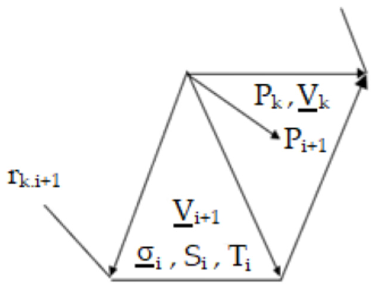
- In the case of 3D domains, we define a mesh of tetrahedra and have the following:whereis the index of the tetrahedron containing the node Pk, is the surface facing outwards, from the i tetrahedron, opposite the node Pk, and Vi is the volume of the i tetrahedron (Figure 5).
- The matrix of system coefficients (39) is sparse non-zero elements on each line corresponding to the neighbouring nodes of the node that defines the line.
2.6. Load Capacity
2.7. Thermal Field Diffusion
2.7.1. Thermal Field Equations, Mathematical Modelling of the Thermal Field during Radio Frequency Heating, and Stationary Regime
Thermal Diffusion
2.7.2. The Finite Element Method and Stationary Regime
The Galerkin Procedure
2.7.3. Discretisation in the Time Domain
- For χ = 0, the explicit Euler method;
- For χ = 1, the implicit Euler method;
- For χ = 1/2, the trapezoidal method.
2.8. Drying of Dielectrics in the Field of Radio Frequency
2.8.1. Model for Solving the Mass Problem
2.8.2. Coupling the Electromagnetic Field and Thermal and Mass Problems
3. Results
- Observations
- The average value of the load temperature;
- The values of the temperature fields;
- The maximum and minimum values of the temperatures in the load and the points where they exit these extremes;
- Humidity;
- Drying time.
Diagram Working
4. Discussion
5. Conclusions
Author Contributions
Funding
Data Availability Statement
Conflicts of Interest
References
- Antti, A.L.; Torgovnikov, G. Microwave Heating of Wood. In Proceedings of the Microwave and High Frequency, International Conferences, Cambridge, UK, 17–21 September 1995; pp. E3.1–E3.4. [Google Scholar]
- Bergman, D.J. The Permitivity of a Simple Cubic Array of Identical Spheres. J. Phys. C Solid State Phys. 1979, 12, 4947. [Google Scholar] [CrossRef]
- Bossavit, A. Uniqueness of Solution of Maxwell Equations in the Loaded Microwave Oven, and How it May Fail to Hold. In Proceedings of the Microwave and High Frequency, International Conferences, Cambridge, UK, 17–21 September 1995; pp. A2.1–A2.4. [Google Scholar]
- Bouirdene, A. Les Fours Thermiques Micro-Ondes. Ph.D. Thesis, INP Toulouse, Toulouse, France, 1992. [Google Scholar]
- Fireţeanu, V. Procesarea Electromagnetică a Materialelor; Editura Politehnica Bucharest: Bucharest, Romania, 1995. [Google Scholar]
- Hobson, L. Basic principles of RF heating, Dielectric Heating Applications. In Proceedings of the Lecture Notes for a Short Course at EEB Staff Training College, Essendon, Australia, 9–13 September 1983. [Google Scholar]
- Leuca, T. Elemente de Teoria Câmpului Electromagnetic. Aplicaţii Utilizând Tehnici Informatice; Editura Universităţii din Oradea: Oradea, Romania, 2002. [Google Scholar]
- Lojewski, G. Microunde. Dispozitive şi Circuite; Editura Teora: Bucharest, Romania, 1996. [Google Scholar]
- Maghiar, T.; Leuca, T.; Bondor, K.; Silaghi, M.; Silaghi, H. Electrotehnică; Editura Universităţii din Oradea: Oradea, Romania, 1999. [Google Scholar]
- Roussy, G.; Pearce, J.A. Foundations and Industrial Applications of Microwave and Radio Frequency Fields. Physical and Chemical Process; John Wiley & Sons Ltd.: Hoboken, NJ, USA, 1995. [Google Scholar]
- Simion, E.; Maghiar, T. Electrotehnică; Editura Didactică şi Pedagogică: Bucharest, Romania, 1981. [Google Scholar]
- Şora, C. Bazele Electrotehnicii; Editura Didactică şi Pedagogică: Bucharest, Romania, 1982. [Google Scholar]
- Wei, J.; Hawley, M.; Asmussen, J. Microwave Power Absorption Model for Composite Processing in a Tunably Resonant Cavity. J. Microw. Power Electromagn. Energy 1993, 28, 234–246. [Google Scholar]
- Bocchi, W.; Grattieri, C. Michelangeli, Numerical Analysis of Electromagnetic Heating: Application to Dielectric Materials. In Proceedings of the International Seminar on Heating by Internal Sources, Padua, Italy, 11–14 September 2001; pp. 301–308. [Google Scholar]
- Brebbia, C.A. Boundary Elements X, Vol.2 Heat Transfer, Fluid Flow and Electrical Applications; Computational Mechanics Publications: Southampton, UK, 1988. [Google Scholar]
- Hănţilă, F.I. Observaţii Asupra Metodei Elementului Finit, Sesiunea de Comunicări Tehnico-Ştiinţifice, I.P.B; Faculty of Electrical Engineering: Bucharest, Romania, 1981; pp. 145–151. [Google Scholar]
- Hănţilă, F.I.; Demeter, E. Rezolvarea Numerică a Problemelor de Câmp Electromagnetic; Research Institute for Electric Machines; Ari Press: Bucharest, Romania, 1995. [Google Scholar]
- Leuca, T.; Bandici, L.; Molnar, C.; Nagy, A. Contributions Regarding the Electric Field Computation in Microwave Owens. In Proceedings of the International Conference RJJSAEM Felix SPA, Oradea, Romania, 11–15 September 2001; pp. 118–124. [Google Scholar]
- Leuca, T.; Bandici, L.; Molnar, C. The Numerical Modeling of Microwave Heating Problems. In Proceedings of the 27th Congress of the Romanian-American Academy of Science and Art and the International Book Fair, 10th Edition, Bucharest, Romania, 26 May 2002; pp. 720–724. [Google Scholar]
- Metaxas, A.C. The use of FE Modelling in RF and Microwave Heating. In Proceedings of the International Seminar on Heating by Internal Sources, Padua, Italy, 11–14 September 2001; pp. 319–328. [Google Scholar]
- Mocanu, C.I. Teoria Câmpului Electromagnetic; Editura Didactică şi Pedagogică: Bucharest, Romania, 1981. [Google Scholar]
- Orfeuil, M. Electric Process Heating; Edition Dunod: Paris, France, 1982; Volume II. [Google Scholar]
- Bialod, M.M.; Marchand, C. La Conception des Installations Industrielles de Chauffage Diélectriques par Haute Frequence et Micro-Ondes, Méthode, Technolojique, Exemples; Electricité de France, Direction des Etudes et Recherches: Paris, France, 1990. [Google Scholar]
- Zhao, H.; Turner, I.W. An Analysis of the Finite-Difference Time-Domain Method for Modeling the Microwave Heating of Dielectric Materials Within a Three-Dimensional Cavity System. J. Microw. Power Electromagn. Energy 1996, 31, 199–214. [Google Scholar] [CrossRef]
- Webb, J.P.; Maile, G.; Ferrari, R. Finite Element Solution of Three-Dimensional Electromagnetic Problems. IEEE Proc. H Microw. Opt. Antennas 1983, 130, 153–159. [Google Scholar] [CrossRef]
- Flux2D, Version 7.1; CAD Package for Electromagnetic and Thermal Analysis using Finite Elements, User’s Guide; CEDRAT: Massy, France, 1994.
- MacGfem. Gfem Documentation Plan; Numerica: Clamart, France, 1988. [Google Scholar]
- Boudrand, H. Introduction au Calcul Electromagnetique des Structures Guidantes; Institut National Polytechnique de Toulouse, ENSEEIHT: Toulouse, France, 1996. [Google Scholar]
- Bandici, L. Modelarea Numerică a Câmpurilor Electromagnetic şi Termic din Instalaţiile Electrotermice cu Microunde. Ph.D. Thesis, University of Oradea, Oradea, Romania, 2003. [Google Scholar]
- Anderson, J.C. Dielectriques; Edition Durand: Paris, France, 1996. [Google Scholar]
- Creţ, R. Contribuţii la Studiul Dielectricilor Neomogeni. Ph.D. Thesis, Technical University of Cluj Napoca, Cluj-Napoca, Romania, 2003. [Google Scholar]
- Helerea, E.; Tiganea, D.; Stanulet, D. Materiale Electrotehnice; Lithography of University of Braşov: Braşov, Romania, 1984. [Google Scholar]
- Leuca, T.; Molnar, C.; Bandici, L.; Nagy, A. Dielectric Materials Properties. Behaviour in the Microwave Field. In Proceedings of the 9th International IGTE Symposium, Graz, Austria, 11–14 September 2000; pp. 413–416. [Google Scholar]
- Nicula, A.; Puşkaş, F. Dielectrici şi Feroelectrici; Editura Scrisul Românesc: Craiova, Romania, 1982. [Google Scholar]
- Robert, P. Matériaux de L’électrotechnique; Presses Polytechniques Romandes: Laussannes, Switzerland, 1989. [Google Scholar]
- Maghiar, T.; Leuca, T. Carmen Molnar, Livia Bandici, The use of finite element in microwave heating. In Proceedings of the Progress in Electromagnetic Research Symposium, Pisa, Italy, 28–31 March 2004; pp. 321–324. [Google Scholar]
- Molnar, C. Contribuţii Privind Modelarea Numerică a Fenomenelor Electromagnetice din Instalaţiile Electrotermice cu Microunde. Ph.D. Thesis, University of Oradea, Oradea, Romania, 2004. [Google Scholar]
- Pichon, L. Finite element analysis of bounded and unbounded electromagnetic wave problems. In Proceedings of the IEE Colloquim on High Frequency Electromagnetic Modelling Techniques, London, UK, 30 March 1995. [Google Scholar]
- Silaghi, M.; Silaghi, H. Tehnologii cu Microunde. Tehnici Informatice; Editura Treira: Oradea, Romania, 2001. [Google Scholar]
- Spoială, D. Numerical modeling of electro-thermal field used for heating spherical dielectric pieces. In Proceedings of the 5th International Conference on Renewable Sources and Environmental Electro-Technologies, Stâna de Vale, Romania, 27 May 2004. [Google Scholar]
- Spoială, D.; Leuca, T. Numerical modelling of electromagnetic and thermal field in wood heating. In Applicator Optimization, Heating by Electromagnetic Sources; Session EF: Padua, Italy, 2004. [Google Scholar]
- Spoială, D.; Leuca, T. Numerical modeling of RF heating spherical rubber pieces. In Applicator Optimization; Simpozionul Naţional de Electrotehnică Teoretică: Bucharest, Romania, 2004. [Google Scholar]
- Bouirdene, A.; Lefeuvre, S. Measurement of thermal and dielectric parameters as function of temperature. In Proceedings of the International Conference, Arnhem, The Netherlands, 26–29 September 1989. [Google Scholar]
- Frandoş, S. Procesarea Materialelor Dielectrice în Câmpuri Electromagnetice de Radio-Frecvenţă şi în Microunde. Ph.D. Thesis, Universitatea Politehnica din București, Bucharest, Romania, 2003. [Google Scholar]
- Keam, R.; Green, A.D. Measurement of Complex Dielectric Permittivity at Microwave Frequencies a Cylindrical Cavity. Electron. Lett. 1995, 31, 212–214. [Google Scholar] [CrossRef]
- Spoiala, D. Modelarea Câmpului Electromagnetic în Regim Cvasistaționar la Înaltă Frecvență. Aplicații la Proiectarea Instalațiilor Electrotermice de Radiofrecvență; Editura Universitatii of Oradea: Oradea, Romania, 2005. [Google Scholar]
- Woode, R.A.; Ivanov, E.N.; Tobar, M.E.; Blair, D.G. Measurement of dielectric loss tangent of alumina at microwave frequencies and room temperature. Electron. Lett. 1994, 30, 2120–2122. [Google Scholar] [CrossRef]
- Jones, P. EA Technology—The Industrial Applications of RF and Microwave Heating, Short Course, Microwave and High Frequency Heating; Capenhurst: Chester, UK, 1995. [Google Scholar]
- Leuca, T.; Maghiar, T.; Silaghi, M.A.; Spoială, D.S. Roman, Numerical analysis of electromagnetic and thermal field in radio frequency applicators. In Proceedings of the 3rd Japan Romania Joint Seminar on Applied Electromagnetics and Mechanical Systems, Felix Spa, Oradea, Romania, 11–15 September 2001; pp. 124–129. [Google Scholar]
- Maghiar, T.; Şoproni, D. Tehnica Încălzirii cu Microunde; Editura Universitatii din Oradea: Oradea, Romania, 2003. [Google Scholar]
- Metaxas, A.C.; Meredith, R.J. Industrial Microwave Heating; Peter Peregrinus LTD (IEE): London, UK, 1983. [Google Scholar]
- Thuéry, J. Les Micro-Ondes et Leur Effets sur la Matiér; Deuxième Edition; Technique et Documentation: Lavoisier, France, 1989. [Google Scholar]
- Avramidis, S. Radio Frequency/Vacumm Drying of Wood. In Proceedings of the International Conference of COST Action El 5 Wood Drying, Ediburgh, Scotland, UK, 13–14 October 1999. [Google Scholar]
- Avramidis, S.; Zwick, R. Exploratory radio frequency/vacumm drying of three D.C. coastal softwoods. Forest Prod. J. 1992, 48, 17–24. [Google Scholar]
- Avramidis, S.; Zwick, R. Comercial scale RF/V drying of softwood timber. Part I, II. Drying characteristics and timber quality. Forest Prod. J. 1996, 46, 27–36. [Google Scholar]
- Beldeanu, E. Produse Forestiere şi Studiul Lemnului; Editura Universitatii Tehnice din Braşov: Braşov, Romania, 2001. [Google Scholar]
- Clemens, M.J. Experience on Radio Frequency dryer for textil fabric webs. In Proceedings of the International Conference, Arhem, The Netherlands, 26–29 September 1989. [Google Scholar]
- Leuca, T.; Spoială, D.S. Roman, Electrotermal installation for processing of the high-frequency electromagnetic field. In Application Consisting of the Wood-Dust Drying in Radio Frequency, Annals of University of Oradea, Romania; Electrotechnical Fascicola; University of Oradea: Oradea, Romania, 2002. [Google Scholar]
- Resch, H.; Gautsch, E. Drying of Lumber in Vacuum using Dielectric Heating, Cost Action E 15, Advances in drying of wood, (1999–2003). Holzforschung und Holzverwertung 2000, 52, 105–108. [Google Scholar]
- Resch, H. High Frequency Heating Continued with Vacuum Drying of Wood. In Proceedings of the 8th International IUFR Wood Drying Conference, Brasov, Romania, 24–29 August 2003; pp. 127–132. [Google Scholar]
- USDA. AirDrying of Lumber; United States Department of Agriculture, Forest Service, Forest Products Laboratory: Washington DC, USA, 1999.
- Leuca, T.; Spoială, D. St. Roman, The Electromagnetic Field Distribution in a Radio Frequency Applicator Used for Poliester Bands Heating; Heating by Internal Sources; Session EF: Padova, Italy, 2001; pp. 365–370. [Google Scholar]
- Simpson, W.; TenWolde, A. Physical Properties and Moisture Relations of Wood, Chapter 3. In Wood Handbook; Forest Products Laboratory, US Department of Agriculture: Madison, WI, USA, 1999. [Google Scholar]
- Torgovnikov, G.I. Dielectric Properties of Wood and Wood Based Materials; Springer: Berlin/Heidelberg, Germany, 1993. [Google Scholar]
- Zhou, B.; Avramidis, S. On the Loss Factor of Wood during Radio Frequency Heating. In Wood Science and Technology; Springer: Berlin/Heidelberg, Germany, 1999; pp. 299–310. [Google Scholar]
- Wood Use. U.S. Competitiveness and Technology; Congres of the United States, Office of Technology Assesment: Washington, DC, USA, 1984; Volume II.
- Wood Handbook, Wood as an Engineering Material; Forest Products Laboratory, U.S. Department of Agriculture: Washington, DC, USA, 1999.
- Grigoraş, G.; Chiruţă, C. Culegere de Probleme de Programare în Limbaj FORTRAN; Lithography of Al. I. Cuza University Iaşi: Iași, Romania, 1977. [Google Scholar]
- Flux2D, Version 7.30; CAD Package for Electromagnetic and Thermal Analysis Using Finite Elements, Dielectrothermal application User’s Guide; CEDRAT: Massy, France, 1998.
- Leuca, T.; Spoială, D. Particularities of the Dielectric Heating in RF; Applicator Optimization; ACTA Academy of Technical Sciences of Romania (Tehnical University of Cluj-Napoca): Cluj-Napoca, Romania, 2006; Volume 47, pp. 153–157. ISSN 1841-3323. [Google Scholar]
- Teodor, L.; Dragoş, S.; Livia, B.; Alexandra, P.P.; Ilie, S. The numerical analysis of electromagnetic and thermal field at the processing of semi-manufactured wood in a RF field. J. Electr. Electron. Eng. 2010, 3, 103–106. [Google Scholar]
- Marcela, L.B.; Dragos, S. Numerical Modeling of The Electromagnetic Field Of Pine Plank In Radio Frequency Heating. J. Electr. Electron. Eng. 2012, 5, 79–82. [Google Scholar]
- Marcela, L.B.; Teodor, L.; Dragos, S. Aspects concerning the heating/drying of oak planks in a radiofrequency field. J. Electr. Electron. Eng. 2013, 6, 59–62. [Google Scholar]
- Dragoș, S.; Constantin, G.N. Aspects regarding the dielectric heating of small wood boards in radio-frequency. J. Electr. Electron. Eng. 2017, 10, 51–54. [Google Scholar]
- Vikberg, T.; Sandberg, D.; Elustondo, D. High Frequency Heating in Solid Wood Modification. In Proceedings of the Seventh European Conference on Wood Modification (ECWM7), Lisbon, Portugal, 10–11 March 2014; pp. 113–114. [Google Scholar]
- Ravindra, V. Gadhave, Radio Frequency Gluing Technique for Wood-to-Wood Bonding: Review. Open J. Polym. Chem. 2023, 13, 15–26. Available online: https://www.scirp.org/journal/ojpchem (accessed on 25 December 2023).
- Tubajika, K.M.; Jonawiak, J.J.; Mack, R.; Hoover, K. Efficacy of radio frequency treatment and its potential for control of sapstain and wood decay fungi on red oak, poplar, and southern yellow pine wood species. J. Wood Sci. 2007, 53, 258–263. [Google Scholar] [CrossRef]
- Leuca, T.; Coman, S.; Trip, N.D.; Bandici, L.; Codrean, M.; Perte, M. Neural Network Modeling of a Drying Process in Radio Frequency Field. In Proceedings of the 15th International Conference on Engineering of Modern Electric Systems, Oradea, Romania, 13–14 June 2019. [Google Scholar]
- Janowiak, J.J.; Szymona, K.S.; Dubey, M.K.; Mack, R.; Hoover, K. Improved Radio-Frequency Heating through Application of Wool Insulation during Phytosanitary Treatment of Wood Packaging Material of Low Moisture Content. For. Prod. J. 2022, 72, 98–104. [Google Scholar] [CrossRef]
- Dubey, M.K.; Janowiak, J.; Mack, R.; Elder, P.; Hoover, K. Comparative study of radio-frequency and microwave heating for phytosanitary treatment of wood. Eur. J. Wood Wood Prod. 2016, 74, 491–500. [Google Scholar] [CrossRef]
- Leuca, T.; Laza, M.; Bandici, L.; Cheregi, G. George Marian Vasilescu, Oana Mihaela Drosu, FEM-BEM Analysis of Radio Frequency Drying of a Moving Wooden Piece. Revue Roumaine de Sciences Technique—Électrotechnique et Énergetique 2014, 59, 361–370. [Google Scholar]


Disclaimer/Publisher’s Note: The statements, opinions and data contained in all publications are solely those of the individual author(s) and contributor(s) and not of MDPI and/or the editor(s). MDPI and/or the editor(s) disclaim responsibility for any injury to people or property resulting from any ideas, methods, instructions or products referred to in the content. |
© 2024 by the authors. Licensee MDPI, Basel, Switzerland. This article is an open access article distributed under the terms and conditions of the Creative Commons Attribution (CC BY) license (https://creativecommons.org/licenses/by/4.0/).
Share and Cite
Spoiala, V.; Silaghi, H.; Spoiala, D. Applied Mathematics in the Numerical Modelling of the Electromagnetic Field in Reference to Drying Dielectrics in the RF Field. Mathematics 2024, 12, 526. https://doi.org/10.3390/math12040526
Spoiala V, Silaghi H, Spoiala D. Applied Mathematics in the Numerical Modelling of the Electromagnetic Field in Reference to Drying Dielectrics in the RF Field. Mathematics. 2024; 12(4):526. https://doi.org/10.3390/math12040526
Chicago/Turabian StyleSpoiala, Viorica, Helga Silaghi, and Dragos Spoiala. 2024. "Applied Mathematics in the Numerical Modelling of the Electromagnetic Field in Reference to Drying Dielectrics in the RF Field" Mathematics 12, no. 4: 526. https://doi.org/10.3390/math12040526
APA StyleSpoiala, V., Silaghi, H., & Spoiala, D. (2024). Applied Mathematics in the Numerical Modelling of the Electromagnetic Field in Reference to Drying Dielectrics in the RF Field. Mathematics, 12(4), 526. https://doi.org/10.3390/math12040526