
The Meaning and Accuracy of the Improving Functions in the Solution of the CBQR by Krotov’s Method

The Department of Civil Engineering, Ariel University, Ariel 40700, Israel
Mathematics 2024, 12(4), 611; https://doi.org/10.3390/math12040611
Submission received: 14 December 2023
/
Revised: 8 February 2024
/
Accepted: 14 February 2024
/
Published: 19 February 2024
(This article belongs to the Special Issue Optimisation Algorithms and Their Applications)
Abstract
:A new solution to the continuous-time bilinear quadratic regulator optimal control problem (CBQR) was recently developed using Krotov’s Method. This paper provides two theoretical results related to the properties of that solution. The first discusses the equivalent representation of the cost-to-go performance index. The second one breaks down this equivalence into smaller identities referencing the components of the performance index. The paper shows how these results can be used to verify the numerical accuracy of the computed solution. Additionally, the meaning of the improving function and the equivalent representation, which are the main elements in the discussed CBQR’s solution, are explained according to the derived notions. A numerical example of structural control application exemplifies the significance of these results and how they can be applied to a specific CBQR problem.
Keywords:
optimal control; Krotov’s method; numerical accuracy; improving function; equivalent representationMSC:
34H05; 93-08; 49N90; 49M991. Introduction
The challenge of “choosing the best path” is a prevalent problem that has a significant presence in applied science and technology [1]. Not surprisingly, its solutions find their way into a wide range of applications, including automatic control of systems [2]. For the latter, the problem is addressed in the framework of optimal control theory. The fundamental objective in this field is to maximize the return from, or minimize the cost of, the operation of physical [3,4], biological [5,6], social [7,8,9], economic processes [10,11], etc.
Many studies have been conducted over the years in optimal control theory, yielding diverse results for many types of problems, and the research is still ongoing. An important tool for solving various optimal control problems is Krotov’s method [2], sometimes referred to by its original name: “a global method of successive improvements of control”. The method, which stems from the fundamental extension principle [2], is a successive algorithm aimed at the computerized solution of optimal control problems. It is a well-known instrument for constructing optimal control for quantum systems [12,13]. Additionally, its efficiency was demonstrated for a class of structural control problems [14,15,16], iron and steel manufacturing processes [17], and biological systems [18].
However, it should be noted that even though Krotov’s method furnishes a rigorous methodology for solving optimal control problems, its formulation is general and requires additional effort when addressing a specific issue. In order to apply the method to a given optimal control problem, one should solve another problem. That is, one should reshape the given performance index to a form that points out a clear way to obtain a better, improved process and the feedback generating it [2]. The reshaped form of the performance index is called an equivalent representation, and the key object for obtaining it is an object called an improving function [2].
One of the recent studies that utilized Krotov’s method deals with the solution for the continuous-bilinear quadratic regulator problem (CBQR) [19]. Here, the aim is to support that solution by furnishing some interesting theoretical comments on the equivalent representation related to this problem. These results can be used to verify the numerical accuracy of the computed improving function and the solution obtained by it. Additionally, in the same context, they shed light on the meaning of the elements of the equivalent representation and the improving function. Section 2 provides some background needed for understanding the main results. The latter are presented in Section 3. Finally, a numerical example is given to illustrate the significance of the results and how they can be used to verify the numerical accuracy of an improving function obtained by the method suggested in [19].
2. Methods
In order to put things in context and facilitate the main derivations, it is beneficial to review several notions and theories.
denotes a state trajectory, and denotes a control trajectory. Here, is an intersection of at t. That is, is a specific vector in that expresses the system’s state at t, whereas refers to the entire trajectory. is a set of control signals admissible to the i-th control device.
The CBQR is an optimal control problem that consists of a bilinear system [20] and a quadratic performance index of the form:
Here, ; and . is a trajectory of external excitations; such that ; such that and . A pair that satisfies Equation (1) is called an admissible process. The set comprises state trajectories, reachable from and the specified . The solution to this problem is required in the form of a state feedback that synthesizes an optimal admissible process, i.e., one that minimizes J.
A successive method was utilized in order to solve this problem [19], that is, to obtain an admissible process that minimizes J. The method, which is named Krotov’s method after its founder Prof. V. F. Krotov [2], furnishes the solution as a sequence called an improving sequence. Krotov defined this sequence to be a sequence of admissible processes——such that ; i.e., the performance of each element in the improving sequence is better than or equal to its former. In addition to this monotonous improvement, the method has the advantages of not being limited to small variations in and obtaining the solution in the form of feedback [2]. A succinct introduction to this method is given below.
Consider a class of optimal control problems defined by a state equation, set of admissible control trajectories, and performance index:
Here, , and . The goal is to find an admissible that minimizes J.
One of the key concepts in Krotov’s theory is the equivalent representation [2]. It was shown that the optimal control problem can be reformulated by transforming the performance index J into an equivalent one, . The rationale behind this transformation lies in the potential for a thoughtfully selected to simplify the solution process. The equivalent representation plays a crucial role in various results put forth by Krotov, notably in Krotov’s method [2]. The subsequent theorem introduces the relevant equivalent representation for our context. and denote vectors in and , respectively.
Theorem 1
([2]). Let be a piecewise-smooth function, upon which the next functions and performance index are constructed:
If is an admissible process, then .
Hence, the challenge is to find a q that forms a beneficial . In the following theorem, Krotov points out a way of finding such a q. The theorem states the properties of q and an improving feedback, , which allow for the improvement of a given admissible process.
Theorem 2
([2]). Let a given be admissible, and let . If the following statements hold:
- 1.
- q grants s and the property:
- 2.
- is a feedbackfor all .
- 3.
- is a state trajectory that solves:at any , and is a control trajectory such that ,
then is an improved process.
A q that meets the requirements listed in the above theorem is called an improving function. By repeating the process improvement over and over, an improving sequence is obtained.
However, while the process of successive improvement proves highly beneficial, this alone does not guarantee optimality. Additional considerations are necessary to ensure that the obtained solution is indeed optimal. For instance, even assuming convergence of the improving sequence, the optimality of its limit process remains uncertain. In the case of an optimum, we anticipatethat it will satisfy conditions of optimality, such as Pontryagin’s minimum principle. Krotov has also addressed this question.
Assume that at some step k of the algorithm, the gradients and are equal for all , and grants the gradient of the following property
at the process . Krotov showed that, in this case, satisfies Pontryagin’s minimum principle with the costate [2]. In this context, Krotov’s method provides a convenient instrument for finding a solution that satisfies Pontryagin’s minimum principle, rather than solving it directly. Furthermore, while solving problems directly via Pontryagin’s minimum principle typically yields an open-loop control trajectory, Krotov’s method offers a solution in a feedback form [21].
The major difficulty faced by a control designer intending to apply Krotov’s method is formulating an improving function suitable for the addressed optimal control problem. For the CBQR problem, given an admissible process, , an improving function can be formulated as [19]. Here, is the solution of the following differential Lyapunov equation [22]:
to , and is the solution of:
to . In these equations, is the control trajectory specified by the given admissible process.
As mentioned above, the improving function q is associated with some , whose importance lies in the fact that it underpins the process improvement. This relation, between the improving function and equivalent representation, is discussed below in Section 3 in the context of the CBQR problem.
3. Results
The equivalent representation of the performance index refers to the entire time domain . However, in some cases, there is an interest in the performance of the system over a sub-interval, , also known as the cost-to-go. Following Theorem 1 one can easily obtain the equivalent representation of the cost-to-go. The next corollary provides an equivalent representation of the cost-to-go of a given admissible process, .
Corollary 1.
Let and be the functionals:
where and is admissible. Then, for any .
The proof is similar to Krotov’s proof to Theorem 1, differing only by setting the time domain to rather than . It is given below for the reader’s convenience.
Proof.
Remark 1.
can be used for evaluating performance over sub-trajectories by:
Assume that is an admissible process. By substituting q into s and then into (Equation (14)), we obtain
Corollary 1 establishes the overall equivalence of J and in a general sense, without delving into their components. The subsequent theorem addresses how this equivalence is reflected through the components of J and for a linear system with an external excitation and no control input, namely:
In brief, the following theorem highlights specific properties of and , which are the solutions to Equations (11) and (12), respectively. These properties allow us to deconstruct the overall equivalence, as described in Corollary 1, into smaller identities. The theorem also provides a tool for verifying the accuracy of and and offers a deeper understanding of their role in .
It is worth noting that, despite the differences between the CBQR and the aforementioned system, the result remains relevant to the CBQR case, as elucidated later in Section 4.
Theorem 3.
Let ; , where . If and satisfy the linear ODEs
for , then:
- (a)
- (b)
- (c)
Proof.
Consider Equations (1) and (2) over , and let . Consequently, Equation (1) becomes:
’s solution consists of homogeneous and particular solutions satisfying Equations (19) and (20), respectively. In addition, Equations (11) and (12) become Equations (21) and (22), repectively.
As is admissible and by Corollary 1:
After substituting :
- (a)
- Let . Hence, , , and
- (b)
- Let . Hence, and
- (c)
- By (a), (b), and cancelling terms from Equation (23):
□
4. Discussion
The fact described in Corollary 1 proves to be useful in certain circumstances. As mentioned earlier, the method proposed for solving the CBQR problem [19] relies on process improvement. However, even though the process is rigorously derived, there is a practical obstacle to its application. The solutions for Equations (11) and (12) are usually obtained through numerical integration methods. In practice, numerical computation errors are always an issue when differential equations are solved numerically [23,24]. Numerical observations show that a successful improvement of a given process——is quite sensitive to the accuracy of q. This accuracy is highly affected by that of and , which solves Equations (11) and (12). Furthermore, differential Lyapunov equations tend to be quite stiff [25,26], making the numerical accuracy issue very present. This is particularly true in the case of Equation (11) and when is rapidly varying or discontinuous, which is a common situation in many practical optimal control problems [2,16,27,28,29]. Therefore, dealing with numerical errors becomes a common practice in the improvement process. As a result, when numerical errors do exist in and , the structure of q becomes flawed and inaccurate, and the improvement might fail. A verification of q’s numerical accuracy at different t’s can be helpful in such a case as it may pinpoint the root of the problem and, consequently, its solution.
First, note that and are specified. Hence they are accurately known, and is accurately known as well. Hence, q’s accuracy at is not of concern. As for q at other t’s, can be used. By taking advantage of the independence of on q, one can verify q’s accuracy at a certain by examining the difference . Clearly, higher accuracy will be reflected in a smaller difference. This tool can be utilized to identify the sections of that contribute to the numerical issues, indicating where additional computational efforts should be focused.
Theorem 3 can be instrumental for a more specific verification of the accuracy of and . Since the right-hand side of expressions (a)–(c) in Theorem 3 depends solely on , it can be computed and compared to the left-hand side of those equations. This allows us to verify the accuracy of the numerically computed and at any given t, as follows.
Throughout the improving steps, the control trajectory undergoes repeated alterations. However, at each step, the previously computed process, say , serves as a fixed starting point. Consequently, at a given step, we treat an admissible control trajectory, , as a specified input. We can now write the state equation for this step as:
where and . Clearly, for the given process, Equation (1) is equivalent to Equation (24). As it is a linear system, the state trajectory can be decomposed into homogeneous and particular solutions. This also applies to each sub-interval . Therefore, over where the homogeneous solution solves
and the particular one, , solves
On the one hand, substituting this decomposition into the CBQR’s l and and then into Equation (13), yields:
On the other hand, according to Equation (18), an admissible process can be evaluated over the sub-interval by:
where and are computed from Equations (11) and (12) to the given and . Obviously, in this case, Equations (21) and (22) solved for and are equivalent to Equations (11) and (12). Theorem 3 reveals that each state-dependent-term on the right-hand side of Equation (27) is equal to a corresponding component of . Let
The above trajectories can be used to verify the accuracy of and ; i.e., according to Theorem 3, a good accuracy should be reflected by a strong agreement in each of the pairs , , and .
Finally, Theorem 3 offers a more profound insight into the meaning of the components in . The identities that are introduced in the theorem reveal that:
- The term evaluates the performance of the homogeneous solution.
- evaluates the performance of the particular solution.
- evaluates the cross-performance of the homogeneous-particular solutions.
Additionally,
This implies that the improving function, q, is a sum of the homogeneous solution’s performance and the cross-performance of the homogeneous-particular solutions.
5. Numerical Example
A CBQR problem that was previously introduced in [19] is used here in order to exemplify an application of the above results. Unlike the original paper, where it was used to demonstrate a practical application of the CBQR problem and its solution, here, the focus is placed on the solution’s numerical accuracy. It illustrates how the above results can be used to verify the numerical accuracy of an improving function that was obtained by the method suggested in [19]. The problem concerns a structural control problem of a two-story building subjected to external excitation and configured with two semi-active variable stiffness (SAVS) devices [30,31]. Devices of this type consist of a frame that connects adjacent floors through a hydraulic element. This element has two operation modes controlled by a servo-valve having two states: open and closed. When the valve is open, it allows almost free flow of the hydraulic fluid, and the device’s resistance to relative floors’ motion is minimal. In a closed state, the valve prevents the fluid’s flow, locks the device, and turns it into a lateral bracing element. Springs and variable dashpots were used for modeling these SAVS devices. Each variable dashpot is capable of providing either a finite or infinite damping, representing the device’s unlocked or locked state, respectively. Figure 1 depicts the dynamic scheme used for modeling the controlled structural system.
The system dynamics amount to the following bilinear state equation:
where the state vector describes the horizontal displacements and velocities in the dynamic degrees of freedom and the forces applied through the SAVS devices to the floors. is the control input trajectory, representing the SAVS devices’ locking patterns. Here, the control policy is restricted to one of three unlocking patterns [30]: (1) both devices are unlocked, (2) only the second device is unlocked, or (3) both devices are locked. These settings lead to an admissible set of control inputs:
Every object in this set reflects the SAVS devices’ unlocking patterns: 1, 2 and 3, respectively. Note that finiteness inhibits variational methods from being used for . A horizontal ground acceleration signal of was used to simulate a seismic excitation.
The performance evaluation accounts for inter-story drifts and control forces. It is:
and were constructed accordingly. It follows that as has no weight in J. Additional details of the system are available in the original paper [19].
Here, that problem is revisited and discussed in the context of Corollary 1 and Theorem 3. That is, in this section, the results are exemplified by demonstrating their application in diagnosing numerical issues emerging during the solution of the above CBQR problem.
Two characteristics of this problem allude that numerical issues are likely to be involved in solving it, especially in solving the differential equations that are related to the process improving stage and the feedback synthesis. First, due to the operation’s principle of the SAVS devices, the control signals are binary. Second, the control signals alternate rapidly. Such issues indeed came up during the CBQR iterations, as follows.
Following [19], Krotov’s method was applied to the CBQR problem through MATLAB. A numerical integration algorithm based on the fourth-order Runge-Kutta method was utilized to solve the necessary differential equations. However, here, computations were carried out twice. In the first case, the integration step was set to , whereas, in the second, it was set to . Notably, even though the fourth-order Runge-Kutta is not recommended for stiff equations [25], it is sufficient for the point discussed in this paper. Here, the discussion revolves around validating the numerical solution’s accuracy rather than its actual accurate computation.
Fifteen iterations were executed, each one consisting of a single CBQR improvement step. As explained above, these iterations generate a sequence of processes, where each is expected to be better than the previous in terms of J. Table 1 provides J’s values, evaluated for each computed process and each case. In this table, i stands for the iteration number. Start with for the initial process, for the process obtained after one improvement, for that obtained after two improvements, and so forth. The table also denotes the relative change in J, signified by .
It can be seen that J’s values in case 2 are different than those of case 1. This implies that the processes, obtained in each case, differ too. Additionally, for an improving sequence, is expected to be non-positive. However, starting at the fifth iteration of case 1, introduces some positive values, which means that a deterioration was obtained rather than an improvement. Although this issue also exists in case 2, it is milder. In case 2, only one such incident was recorded—after iteration 13. The explanation to this non-monotonous behavior is numerical errors, involved in the computation of and . Obviously, case 2, which benefits from higher accuracy due to a smaller integration step, is more reliable than case 1.
Hence, inspection of the monotonicity of can serve as a simple measure of the accuracy of the obtained process. Nevertheless, a deeper inspection can be performed through a comparison of the original cost-to-go with its equivalent counterpart, which was defined in Corollary 1, . Such a comparison is presented in Figure 2. In this figure, case 1’s costs are , , and case 2’s are , . Corollary 1 states that, theoretically, and should be identical for any . However, this property is not observed in case 1. It can be seen that substantially deviates from . In contrast, in case 2, there is a relatively good agreement between and . Additionally, Figure 2 points out another interesting fact. It can be seen that and are not equal. Although they do have similar initial and terminal costs, they differ over the majority of time instances. This is another sign of the difference between the solutions obtained in case 1 and 2. However, the good agreement of and implies that case 2 is the accurate one.
Can we better identify the reason for the poor performance of case 1? Based on Theorem 3, the answer is yes. Consider the identities defined in Theorem 3 and the terms defined in Equation (28). A better identification can be obtained by examining the equivalence of the terms in each one of the pairs: , , and .
Figure 3 inspects this equivalence in each case. As before, a ‘c1’ superscript indicates case 1, and case 2 is indicated by ‘c2’. The correspondence in each of the pairs is conspicuous in case 2. However, even though case 1 shows reasonable similarity in the two first pairs, in the third pair, is dissimilar to for . It follows that in the given problem this element is the reason for the difference between and . Because the pair consists of , which is absent from the other pairs, it is suggested that the numerical obstacle in the given problem is most likely related to the components of , i.e., either the control input , the external excitation , or both.
6. Conclusions
This paper furnishes novel theoretical results that are related to a recently published solution to the CBQR problem. Specifically, the results refer to a key element in that solution—the improving function. First, Corollary 1 defines an equivalent cost-to-go performance index. Notably, its formulation is general and not limited to the CBQR problem. A sub-interval’s equivalence is an immediate consequence of this theorem and is discussed too. Next, Theorem 3 continues the idea presented in Corollary 1 but concentrates on the CBQR case.
The theorem breaks the equivalence down into smaller identities in relation to the components of the CBQR improving function.
These results allow us to verify the accuracy of the obtained numerical solution. This can be performed for the overall accuracy of the computed feedback and each of its components. It is an important tool as numerical issues frequently arise in solving ODEs, especially when discontinuous control signals and excitations are involved. Additionally, these theoretical results shed light on the meaning of the equivalent representation, the improving function, and the way in which they are related to the given problem.
A numerical example from structural control is provided to illustrate the above identities and how they can be used to verify the accuracy of the computed solution and pinpoint causes of inaccuracy, if there are such.
Based on the above results, different future research directions can be considered. The following are three possible directions. First, the results were demonstrated to have application in validating the numerical accuracy of improving functions. However, there is still work to be performed on systematically incorporating such a validation into the iteration process and what steps should be taken when errors are encountered. Second, can the identities from Theorem 3 be extended for more complex systems? Third, the derived identities provide novel explanations of the elements of the improving function related to the CBQR problem. It would be beneficial to examine their utilization in improving the computation time and effort required to solve that problem.
Funding
This research received no external funding.
Data Availability Statement
No new data was created or analyzed within the manuscript.
Conflicts of Interest
The author declares no conflict of interest.
Abbreviations
The following abbreviations are used in this manuscript:
| CBQR | Continuous-Time Bilinear Quadratic Regulator |
| ODE | Ordinary Differential Equation |
References
- Gerdts, M. Optimal Control of ODEs and DAEs; De Gruyter Oldenbourg: Berlin, Germany; Boston, MA, USA, 2024. [Google Scholar] [CrossRef]
- Krotov, V.F. Global Methods in Optimal Control Theory; Chapman & Hall/CRC Pure and Applied Mathematics; Taylor & Francis: Boca Raton, FL, USA, 1995. [Google Scholar]
- Wu, K.; Ren, C.; Chen, Y. An optimal control method for time-delay feedback control of 1/4 vehicle active suspension under random excitation. J. Low Freq. Noise Vib. Act. Control 2022, 41, 732–747. [Google Scholar] [CrossRef]
- Safiullah, S.; Rahman, A.; Ahmad Lone, S. Optimal control of electrical vehicle incorporated hybrid power system with second order fractional-active disturbance rejection controller. Optim. Control Appl. Methods 2021, 44, 905–934. [Google Scholar] [CrossRef]
- Lunz, D.; Bonnans, J.F.; Ruess, J. Optimal control of bioproduction in the presence of population heterogeneity. J. Math. Biol. 2023, 86, 43. [Google Scholar] [CrossRef]
- Lamwong, J.; Wongvanich, N.; Tang, I.M.; Pongsumpun, P. Optimal Control Strategy of a Mathematical Model for the Fifth Wave of COVID-19 Outbreak (Omicron) in Thailand. Mathematics 2024, 12, 14. [Google Scholar] [CrossRef]
- Ibrahim, O.; Okuonghae, D.; Ikhile, M. Optimal control model for criminal gang population in a limited-resource setting. Int. J. Dyn. Control 2023, 11, 835–850. [Google Scholar] [CrossRef] [PubMed]
- Sahoo, B.; Das, R. Crime population modelling: Impacts of financial support. Int. J. Dyn. Control 2023, 11, 504–519. [Google Scholar] [CrossRef]
- Jain, A.; Dhar, J.; Gupta, V.K. Optimal control of rumor spreading model on homogeneous social network with consideration of influence delay of thinkers. Differ. Equ. Dyn. Syst. 2023, 31, 113–134. [Google Scholar] [CrossRef]
- Kirk, D.E. Optimal Control Theory: An Introduction; Dover Publications: Miniola, NY, USA, 2004; p. 479. [Google Scholar]
- Cadenillas, A.; Huamán-Aguilar, R. The Optimal Control of Government Stabilization Funds. Mathematics 2020, 8, 1975. [Google Scholar] [CrossRef]
- Morzhin, O.; Pechen, A. Krotov method for optimal control of closed quantum systems. Russ. Math. Surv. 2019, 74, 851–908. [Google Scholar] [CrossRef]
- Fernandes, M.E.F.; Fanchini, F.F.; de Lima, E.F.; Castelano, L.K. Effectiveness of the Krotov method in finding controls for open quantum systems. J. Phys. A Math. Theor. 2023, 56, 495303. [Google Scholar] [CrossRef]
- Halperin, I.; Agranovich, G.; Ribakov, Y. Using Constrained Bilinear Quadratic Regulator for the Optimal Semi-Active Control Problem. J. Dyn. Syst. Meas. Control 2017, 139, 111011. [Google Scholar] [CrossRef]
- Halperin, I.; Agranovich, G.; Ribakov, Y. Multi-input control design for a constrained bilinear biquadratic regulator with external excitation. Optim. Control Appl. Methods 2019, 40, 1045–1053. [Google Scholar] [CrossRef]
- Halperin, I.; Agranovich, G.; Ribakov, Y. Design of Optimal Feedback for Structural Control; CRC Press: Boca Raton, FL, USA, 2021. [Google Scholar]
- Liu, Y.; Zhou, P. Optimal tracking control for blast furnace molten iron quality based on subspace identification and Krotov’s method. Optim. Control Appl. Methods 2023, 44, 2532–2550. [Google Scholar] [CrossRef]
- Halperin, I.; Agranovich, G.; Lew, B. The Discrete Bilinear Biquadratic Regulator. IEEE Trans. Autom. Control 2021, 66, 5006–5012. [Google Scholar] [CrossRef]
- Halperin, I. Solution of the Continuous Time Bilinear Quadratic Regulator Problem by Krotov’s Method. IEEE Trans. Autom. Control 2023, 68, 2415–2421. [Google Scholar] [CrossRef]
- Bruni, C.; DiPillo, G.; Koch, G. Bilinear systems: An appealing class of “nearly linear” systems in theory and applications. IEEE Trans. Autom. Control 1974, 19, 334–348. [Google Scholar] [CrossRef]
- Krotov, V.F. A technique of global bounds in optimal control theory. Control Cybern. 1988, 17, 115–144. [Google Scholar]
- Gajic, Z.; Qureshi, M.T.J. The Lyapunov Matrix Equation in System Stability and Control; Academic Press, Inc.: Cambridge, MA, USA, 1995. [Google Scholar]
- Gimeno, J.; Jorba, À.; Jorba-Cuscó, M.; Miguel, N.; Zou, M. Numerical integration of high-order variational equations of ODEs. Appl. Math. Comput. 2023, 442, 127743. [Google Scholar] [CrossRef]
- Ji, Y.; Xing, Y. Highly Accurate and Efficient Time Integration Methods with Unconditional Stability and Flexible Numerical Dissipation. Mathematics 2023, 11, 593. [Google Scholar] [CrossRef]
- Shampine, L.F.; Gear, C.W. A User’s View of Solving Stiff Ordinary Differential Equations. SIAM Rev. 1979, 21, 1–17. [Google Scholar] [CrossRef]
- Choi, C.H. Solving stiff Lyapunov differential equations. In Proceedings of the 2000 American Control Conference, ACC (IEEE Cat. No. 00CH36334), IEEE, Chicago, IL, USA, 28–30 June 2000; Volume 5, pp. 3370–3372. [Google Scholar]
- Adhyaru, D.M.; Kar, I.N.; Gopal, M. Constrained Optimal Control of Bilinear Systems Using Neural Network Based HJB Solution. In Proceedings of the 2008 IEEE International Joint Conference on Neural Networks (IEEE World Congress on Computational Intelligence), Hong Kong, China, 1–8 June 2008; pp. 4137–4142. [Google Scholar] [CrossRef]
- Hassan, M.; Boukas, E. Constrained linear quadratic regulator: Continuous-time case. Nonlinear Dyn. Syst. Theory 2008, 8, 35–42. [Google Scholar]
- Liu, C.; Loxton, R.; Teo, K.L. A Computational Method for Solving Time-Delay Optimal Control Problems with Free Terminal Time. Numer. Algebra Control Optim. 2014, 72, 53–60. [Google Scholar] [CrossRef]
- Kobori, T.; Takahashi, M.; Nasu, T.; Niwa, N.; Ogasawara, K. Seismic response controlled structure with Active Variable Stiffness system. Earthq. Eng. Struct. Dyn. 1993, 22, 925–941. [Google Scholar] [CrossRef]
- Zoccolini, L.; Bruschi, E.; Cattaneo, S.; Quaglini, V. Current Trends in Fluid Viscous Dampers with Semi-Active and Adaptive Behavior. Appl. Sci. 2023, 13, 10358. [Google Scholar] [CrossRef]
Figure 1.
Dynamic scheme for a two-floor structure, equipped with two SAVS devices [19].
Figure 1.
Dynamic scheme for a two-floor structure, equipped with two SAVS devices [19].
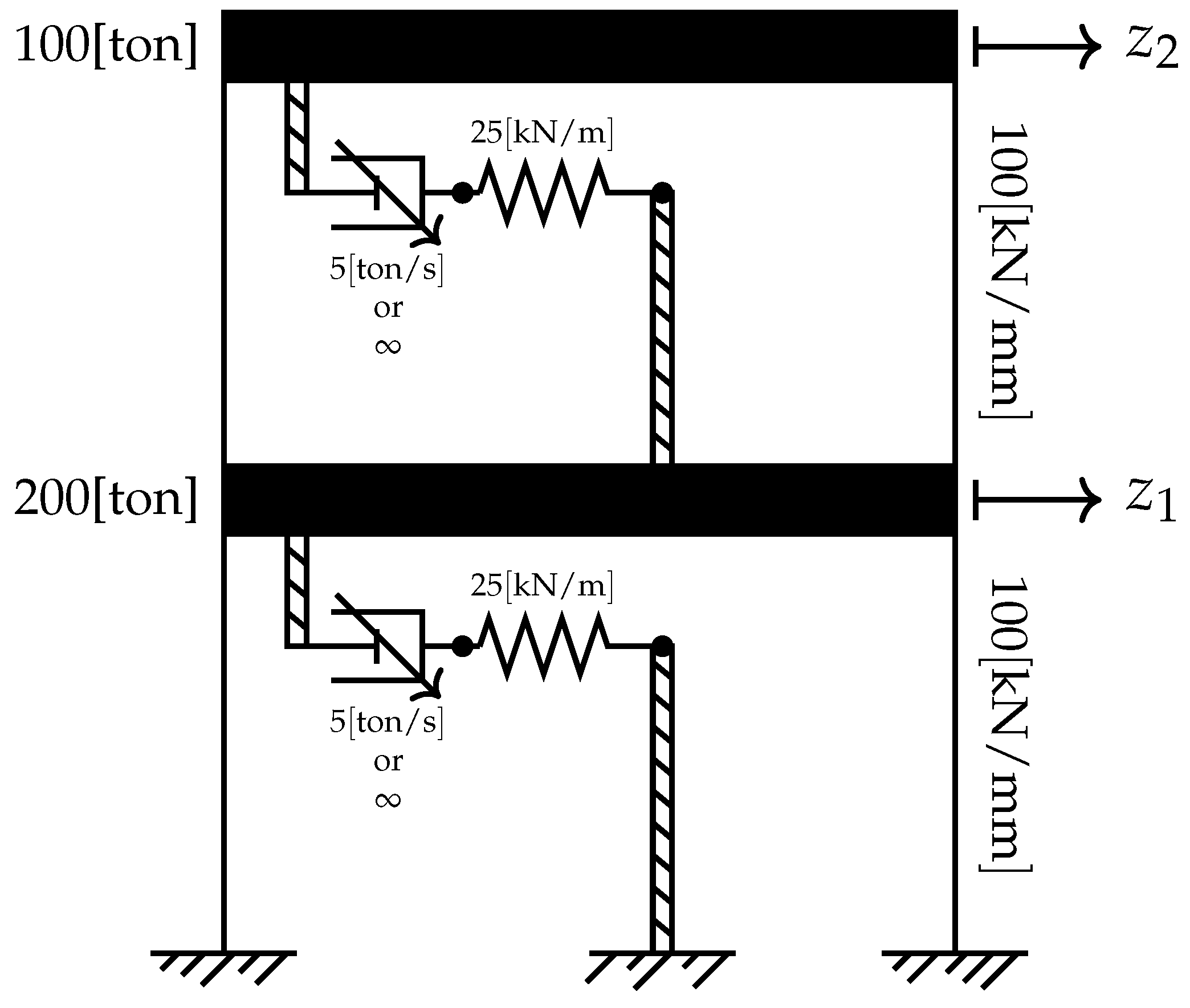
Figure 2.
Cost-to-go trajectories in case 1 (,) and case 2 (,).

Figure 3.
Trajectories of the cost-to-go elements for cases 1 and 2: (a) against , (b) against , (c) against . Case 1 is indicated by a superscript and case 2 is indicated by a superscript.
Figure 3.
Trajectories of the cost-to-go elements for cases 1 and 2: (a) against , (b) against , (c) against . Case 1 is indicated by a superscript and case 2 is indicated by a superscript.


Table 1.
Peformance index values at each process. Here, .
| Case 1 | Case 2 | |||
|---|---|---|---|---|
| 0 | - | - | ||
| 1 | ||||
| 2 | ||||
| 3 | ||||
| 4 | ||||
| 5 | ||||
| 6 | ||||
| 7 | ||||
| 8 | ||||
| 9 | ||||
| 10 | ||||
| 11 | ||||
| 12 | ||||
| 13 | ||||
| 14 | ||||
| 15 | ||||
Disclaimer/Publisher’s Note: The statements, opinions and data contained in all publications are solely those of the individual author(s) and contributor(s) and not of MDPI and/or the editor(s). MDPI and/or the editor(s) disclaim responsibility for any injury to people or property resulting from any ideas, methods, instructions or products referred to in the content. |
© 2024 by the author. Licensee MDPI, Basel, Switzerland. This article is an open access article distributed under the terms and conditions of the Creative Commons Attribution (CC BY) license (https://creativecommons.org/licenses/by/4.0/).
Share and Cite
MDPI and ACS Style
Halperin, I. The Meaning and Accuracy of the Improving Functions in the Solution of the CBQR by Krotov’s Method. Mathematics 2024, 12, 611. https://doi.org/10.3390/math12040611
AMA Style
Halperin I. The Meaning and Accuracy of the Improving Functions in the Solution of the CBQR by Krotov’s Method. Mathematics. 2024; 12(4):611. https://doi.org/10.3390/math12040611
Chicago/Turabian StyleHalperin, Ido. 2024. "The Meaning and Accuracy of the Improving Functions in the Solution of the CBQR by Krotov’s Method" Mathematics 12, no. 4: 611. https://doi.org/10.3390/math12040611
Note that from the first issue of 2016, this journal uses article numbers instead of page numbers. See further details here.