Abstract
Ecotourism routes serve as powerful tools for fostering environmental awareness. To achieve this, it is crucial to design itineraries within natural parks that strike a balance between visitor experience and ecological preservation. Limiting the duration of visits prevents undue strain on both visitors and ecosystems. Effective routes should showcase high biodiversity, traversing diverse sites to enhance knowledge acquisition. Considering natural factors such as light conditions and climate, it is prudent to tailor visiting times to optimize the experience. Therefore, it makes sense to incorporate time-dependent benefits at arcs and the possibility of introducing waiting times at nodes in the design models. These two characteristics have enriched the optimization models developed to solve the tourist trip design problem based on maximizing benefit only when points of interest are visited. However, the specific application of these aforementioned characteristics and enriched optimization models to the arc orientation problem remains yet to be reported on and published in the literature. Our contribution addresses this gap, proposing a route design model with scenic value in the arches of the graph where the benefits perceived by travelers are maximized, taking into account a diversity of evaluations depending on the time of starting the trip through each arc.
Keywords:
tourist trip design problem; arc orienteering problem; scenic path; tourist preference; ecotourism route MSC:
90B06
1. Introduction
The tourism trip design problem (TTDP) consists of selecting a subset of places to visit (points of interest, POIs) from a larger set of options with the objective of maximizing the benefit perceived by the tourist during that sequential tour. The benefit is expressed algebraically by means of the sum of individual rewards generated at each location visited. There are a series of restrictions to impose in the search for solutions that have been discussed extensively in the literature: limited budget, time windows established in the places visited, maximum trip duration, etc. [1]. From a scientific point of view, the formulation of the TTDP is based on an adaptation of the Orienteering Problem (OP), that is the problem of finding a tour that maximizes the profits collected at the vertices and that the cost of the trip does not exceed a certain value. This approach could be considered as a generalization of the Knapsack problem, where the travel time and budget are two constraints to be satisfied [2]. There are a large number of studies OP [3,4,5,6]. A survey of the TTDP can be found in [7]. A review of algorithms proposed to solve the TTDP can be found in [8].
In order to plan the travel itinerary for a tourist visiting a city over a set period of time, it is necessary to have prior knowledge of the location of several POIs in a transportation network, as well as to estimate the tourist’s satisfaction values for each one of those POIs and their characteristic attributes (e.g., opening/closing times, estimated duration of the visit, cost of the visit, specific categories to which the POI belongs, etc.). In addition, the tourist can impose other particular restrictions, such as the amount of money he/she plans to spend on the tour and the maximum number of points of interest of a certain type/category that he/she is willing to visit [6].
As mentioned above, the objective function consists of maximizing the global benefit of the tourist package by determining an optimal sequence of exploring attractive sites. An added complexity consists of considering that the objective function is dynamic, since the preferences of different tourists may vary according to different visit times. In this context, Erdogan and Laporte (2013) [9] studied a variant of the OP, namely the OP with Variable Profits (OPVP); ref. [10] extended the model by considering that the profit of each node may be a decreasing function of time. Recently, new features have been considered that enrich the optimization models developed; for example, to assume that the benefit derived from the visit to each POI is dependent on the time of day in which it is carried out and, consequently, being able to include the opportunity to modify the departure in the model from a POI to obtain a greater benefit along its exit arc [11,12].
A minimum spanning tree (MST) is a method of connecting all the vertices of a graph in a way that minimizes the total weight of the edges of the tree. When the nodes in the graph represent transportation nodes, then a minimal spanning tree can suggest a least-cost (or near-least-cost path) through all nodes in the graph. This tool can be very useful when designing a tour made up of different places to visit. An MST-based algorithm can reduce the amount of time needed to determine a route and also increase traveler confidence in the suggested route. In Gao et al. (2018) [13], a tourism resources planning is proposed, based on adaptive minimum spanning tree models combined with a fuzzy level evaluation method, to effectively divide tourism agglomeration areas to support tourism-planning decision.
In addition to adaptations of classic optimization models, other heuristics and metaheuristics have contributed to the effective planning of tourist routes. In Damos et al. (2021) [14], the traditional multi-objective genetic algorithm was improved by previously adding an Analytic Hierarchy Process (AHP) in two phases to more accurately determine the weights of objectives considered and to produce more straightforward solutions addressed to develop tourism path planning. The proposed approach has been experienced on the tourist road network around Chengdu City in China. In Suanpang et al. (2022) [15], a hybrid genetic algorithm, combined with a simulated annealing algorithm, was applied over data from Thailand’s tourism industry to create schedules for tourism services, in accordance with the preferences of tourists.
Complementarily, in the Arc Orienteering Problem (AOP), the benefits perceived by the traveler are associated with trips through the edges/arcs of the graph, instead of the visits made to its vertices. This problem is a well-known NP-hard combinatorial optimization problem [8]. This model has already been successfully applied in the tourism field to calculate personalized walking routes in historic cities [1,16,17], bicycle itineraries [18] and ecotourism routes in Nature Parks [19].
Like the traditional OP, the AOP models try to find a route connecting two points in a network, where the total benefit is maximized without violating the established constraints. The Orienteering Tour Problem (OTP) is a specific version where the starting and ending nodes of the tour are identical [20,21]. In the Bus Sightseeing Problem (BSP), there are two interconnected decision levels: The assignment of tourists to buses and the design of routes of buses to visit various attractions [22]. Deitch and Ladany (2000) [23] define an orienteering problem (namely, the Bus Touring Problem, BTP) where the objective is to design the route of a tourist bus that maximizes the “attractiveness” of the sites to visit and the scenic value of the route traveled. Feillet et al. (2005) [24] propose a branch-and-price approach for the profitable arc tour problem.
There are several studies that examine identifying a scenic path that is focused on the scenic attractiveness along arcs instead of the attractiveness values associated with the nodes [25,26,27]. Based on the previous existence of candidate lines, Ning et al. (2022) [28] propose offline (trip generation and assignment algorithm) and online (passenger assignment algorithm based on arrival data) algorithms to solve the Bus Scheduling and Route Planning (BSRP) problem. Extensive experiments based on a real-world data set from Shanghai (China) were conducted to test the effectiveness of such heuristics in terms of route length, average number of passengers, and number of buses required.
For instance, Quercia et al. (2014) proposed a probability model to calculate the “emotional” score on the route based on the crowdsourced people’s perceptions [27]. They studied the problem of finding a path from an origin O to a destination D subject to two constraints: the path should be short and the total value is maximized. To this aim, they developed a two-phase algorithm: (1) find the top-k shortest paths from node O to node D; and (2) among such paths, find the one along which a higher emotional score is produced.
In a similar vein, Zheng et al. (2013) also studied the problem of finding the shortest path where the scenic score, due to the observed landscape, is maximized [25]. To solve this problem, the authors developed an algorithm that transforms the existing road network G to a “scenic” network , where all nodes on the new graph accumulate weights associated with the scenic values derived from their landscape environment. This problem can then be easily solved by finding the shortest path in . As previously pointed out, the problem of finding the most scenic path, while keeping the total travel cost within a specific budget, can be formulated as a variant of AOP which is an NP-hard combinatorial optimization problem. This is the motivation for developing a series of meta-heuristic algorithms capable of solving the problem, generating a rapid response in large-scale road networks.
The search for optimal solutions in the strict sense can be made more flexible since the user of a sightseeing experience may often be willing to take a longer scenic path, as long as the travel time (or budget) of the path is within their personal restrictions.
When an integer optimization problem is formulated with two objective functions (say, profit and diversity) that have to be optimized simultaneously, it is common to generate the set of Pareto-optimal solutions. A route solution R is Pareto-optimal if there does not exist another solution S that dominates R, in the sense that S has at least the same profit and at most the same diversity as R and at least one of these inequalities is strict. The optimal solution to this bi-objective problem is the set of Pareto-optimal solutions not exceeding the budget in terms of traveled time or cost. Corley and Moon (1985) [29] developed an enumerative approach based on label correcting for determining shortest paths in networks with vector weights. Ref. [30] present a classification of the existing algorithms for the bicriterion shortest-path problem ranked by computational performance. Multi-objective problems can generate different shapes of Pareto optimal fronts (POF) with geometric characteristics (convexity, linearity, separability, etc.) that exhibit certain weaknesses for guaranteeing the quality of the solution. Zheng et al. (2023) [31] generated a better diversity of solutions in the Pareto layering structure by crossing and mutating between adjacent domains and decomposing the multi-objective problem into multiple neighborhood subproblems.
If a route that is optimal for a certain criterion (say, for example, it minimizes the total distance traveled), does not exhibit a competitive value for another of the criteria, it is advisable to analyze the efficiency of other alternative feasible routes orderly following the suboptimal value reached. In this context, K-shortest path problems (KSP) models take care of finding an orderly collection of suboptimal paths, from the first shortest path to the k-th shortest path, between an origin–destination pair in the network [32,33]. KSP problems have been intensively researched due to the breadth and versatility of their applications. In particular, KSPs represent a useful tool when providing routes to satisfy multiple objectives [34], with different constraints [35,36] or considering several preferences that different users may have before choosing the route [37].
Lindberg and Hawkins (1993) [38] define the term ecotourism as responsible travel to visit natural areas where the environment is conserved while improving the well-being of the local population. Ecotourism destinations have increased worldwide. The routes designed for this purpose help visitors acquire greater sensitivity and awareness about environmental values, especially in school-age children. Various authors warn about the undesirable effects of deterioration of the natural environment that may arise due to unrestricted tourism [39,40]. To protect the environment from such harmful impacts, it is recommended that the duration of an itinerary should not exceed a certain threshold so that its completion does not require significant effort for people and that the ecosystem is not affected. Finally, the route design must also try to incorporate a high level of biodiversity [41].
In this article on the design of ecotourism routes, with time-dependent benefits along the arcs and the possibility of strategically establishing waiting times, several characteristics have been analyzed:
- 1.
- The existence of attractiveness in the arcs that can be time-dependent, according to the starting time for the route section in question.
- 2.
- The opportunity to establish a delay in the exit node towards the new arc to travel in order to obtain greater profitability.
- 3.
- Enrichment of the diversity of typologies assimilated by the traveler along the route to be determined.
In this paper, the tourist trip design problem (TTDP) with constraints typical of ecotourism routes (limiting the trip duration, starting and ending at the same point, promoting the range of observed types along the path) is analyzed. The decision space for solutions consists of a transformed graph extracted from the original transportation network, by adding new nodes and new arcs to integrate into the model the possibility of waiting times at the nodes before continuing the trip with the expectation of producing a greater emotional benefit for the visitor. The proposed framework is an Integer Linear Programming (ILP) model. Due to the computational inefficiency in solving large-scale instances with a commercial ILP solver, a heuristic is then developed and its pseudocode provided. In total, two computational experiences are implemented and their obtained results are discussed.
The remainder of the paper is organized as follows: Section 2 formulates the proposed mathematical model and develops an algorithm to ensure that the arcs with the highest benefit value for various types can be preferentially selected for inclusion in the optimal route. Section 3 describes two computational experiences on transport networks inspired by those currently operating in Andalusia and Portugal/Spain. Finally, Section 4 is dedicated to concluding remarks and future work.
2. Problem Formulation
2.1. Problem Description
Let us represent by the graph associated to the transport network, composed of the set V of n nodes and the set A of arcs. Every arc can be represented by the ordered pair () of starting and ending nodes. Let us distinguish by O the origin node of the trip and by D the destination node.
Let be the travel time between nodes i and j along arc () ∈ A. By reiteratively applying the Dijkstra Algorithm [42], a vector f that records the minimum travelling costs toward the origin O from each other node of G can be built. Let be the minimum travel cost between nodes O and .
Assume that a special interest for the traveler could be located both along arcs as at vertices. Therefore,
- Let be the attractiveness score, perceived by the tourist, when he/she travels along arc . The route attractive qualities could be, as was recorded in the National Scenic Byways Program [43], scenic, recreational, natural, cultural, historical, or archaeological, for instance.
- Let be the profit acquired by travelers when visiting node . The interest of staying at node i can be motivated by a cultural visit of that site or, simply, to meet relaxing experience.
Both parameters and must be non-negative. Additionally, it will be assumed that the attractiveness of the route along the arc (i.e., the value of parameter ) will depend on the start time at node i (for example, sunlight or the level of the tides can determine the scenic value of the landscape).
Therefore, the form of varying parameter will be assumed to be a step function that changes its value along time t at certain instants (increasing or decreasing) and remains at that level until the next milestone. That is, the attractiveness score is time dependent. The parameters and must have a normalized valuation range that allows the sum of the individual rewards to evaluate the objective function.
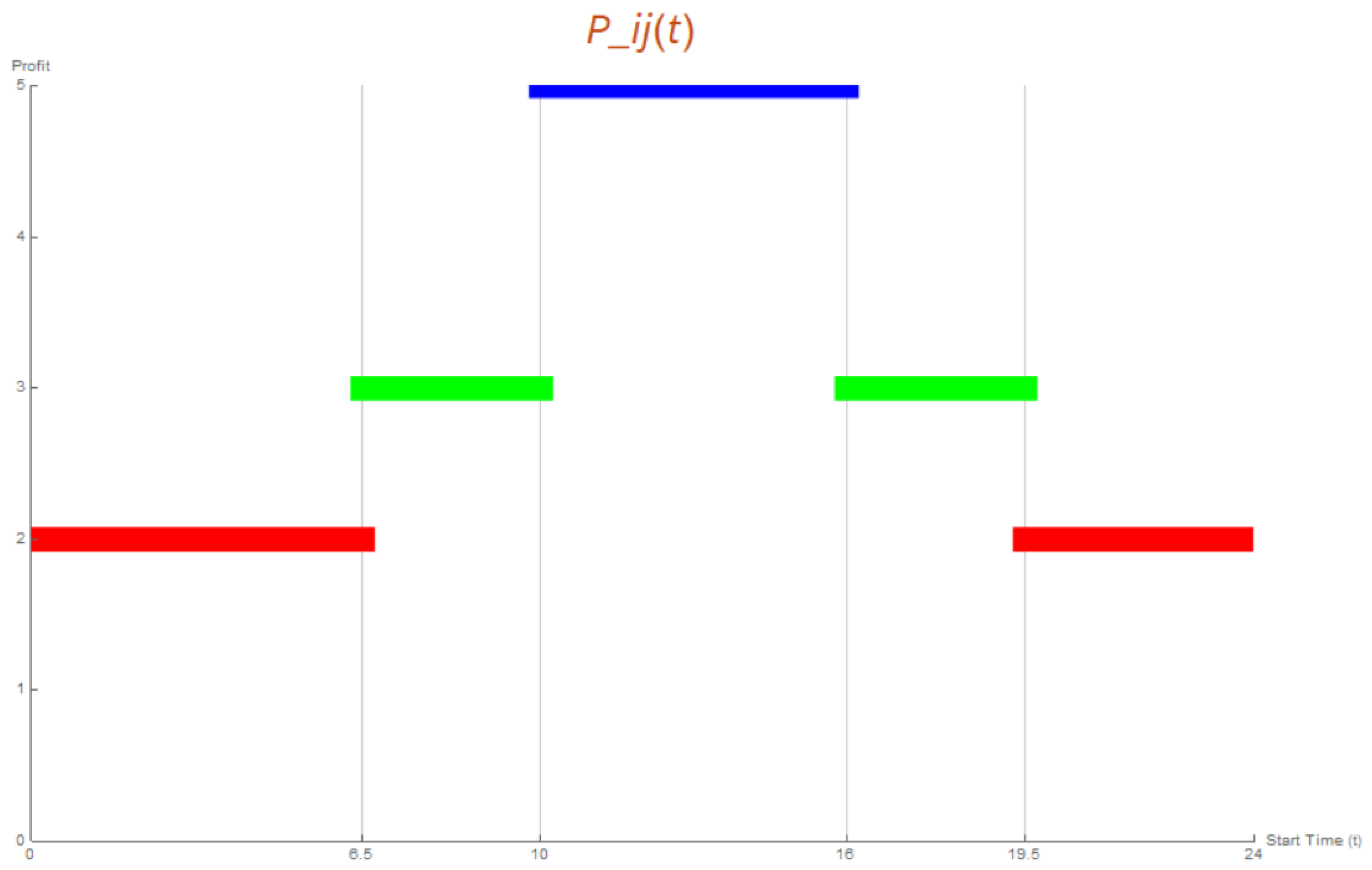
Travel along the arc implies that the route first passes through node i and, after a time , reaches node j. The times in which the visit to the nodes occurs can condition the opportunities that travelers have to enjoy the specific places of interest associated with each node, so it is relevant to emphasize that the graph, as a solution space, must be assumed directed by default. In Figure 1, has graphically been represented an example of a step function that indicates several levels for the attractiveness score, perceived when traversing the arc . The step function in Figure 1 shows a basic level of attractiveness (profit = 2, in red) when the arc is traversed. This score increases (profit = 3, in green) if the visit is carried out during daylight hours (interval [6.5, 19.50]), and finally, the benefit perceived by the traveler especially increases (profit = 5, in blue) when that visit occurs during business opening hours (interval [10, 16]). This function format has already been used in the literature that analyses the route efficiency in networks with time-dependent arcs.
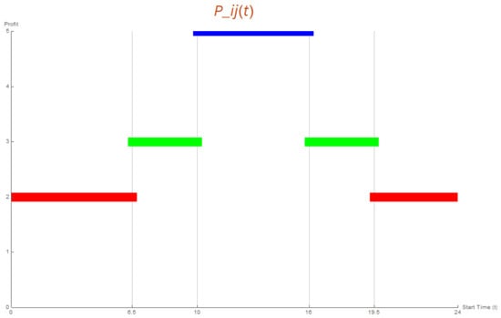
Figure 1.
Instance of step function describing .
Two issues must be solved prior to making a proposal for the formulation of an optimization model for route determination:
- 1.
- Graphically represent the free option of traveler to be able to wait a period of time at node i, with the strategic objective of increasing the profit value of the arc after the waiting period.
- 2.
- Manage the possibility of taking advantage of the visit to node i (that is, incorporating the value to the objective) whenever the route runs through said node.
The first question can be resolved in the way proposed in [44]. In order to adequately manage the multiplicity of attractiveness values in each arc we must replicate node i as many times as the number of differentiated levels have been considered for the arc . Some of these levels may be ignored when their validity is outside the temporal domain established by the earliest arrival time at node i. Replicas of node i may be aligned vertically in a sequential way and be labelled as , etc. For a greater level of detail, we refer to the article by [44].
The second question can be resolved by additively accumulating the value in each of the incoming arcs , adding it with the attractiveness due to the arc. To avoid duplication in the computation of the weights, the restriction that the feasible path could only once pass through any of the nodes of V should be included in the model. For a greater level of detail on how to assign vertex weights to its adjacent arches, we refer to the article by [19]. For better understanding:
Let be a time value that produces the first change of level in the attractiveness of the arc . Let us assume that , for ; ; , for . In this context, node i will be replaced by the vertical sequence of nodes:
- : geographically located in the same place as the original node i, and maintaining the same connections through arcs with the neighbouring nodes established in the graph G. The attractiveness values of these arcs are not modified. That is, the attractiveness value of arc will be a. Moreover, the minimum travel cost between nodes O and does not change: .
- : geographically located above the node , and maintaining the same connections through arcs with the neighbouring nodes as the preceding node . The attractiveness value of arc will be b. Additionally, a new arc will be built that will have an associated travel time (actually, waiting time) and whose attractiveness will correspond to the value established as a consequence of the visit to node i (that is, ). Logically, the minimum travel cost between nodes O and changes: .
- [generated as a consequence of a second change of level at ()]: this new node will also be located on the vertical of the node , and will maintain the same connections through arcs with the neighbouring nodes as the preceding node . The attractiveness value of arc will be c. Additionally, a new arc will be built that will have an associated travel time (the additional waiting time) and whose attractiveness value will be considered null to avoid double counting of benefits in the visit to node i. The minimum travel cost between nodes O and is updated:
Once the graph that contains the possible solutions has been built, the problem can be modeled as follows: A tourist starts their trip from a predefined initial location O and must arrive at a predefined destination D, through a route where the collected profit is maximized and such that the travel cost does not exceed a given value T. The value of parameter T must be adjusted to the time that is considered reasonable in completing the route, avoiding fatigue or discomfort for the tourist.
In order to avoid a cumbersome notation in the mathematical formulation, let us rename the graph of solutions as at the beginning. Let, then, be the graph associated to the transport network.
2.2. Mathematical Model
To model the problem as a mixed integer linear program model, we use two sets of variables.
- The first type of binary variables, , is 1 if a visit to site i is followed by a visit to site j, and 0 otherwise.
- The second type of binary variables, , takes the value 1 (0) if node i is (not) selected to be in the route.
Additionally, let denote the set of arcs incident with node i. This notation can be extended to any set of vertices : . Finally, let introduce an operator that computes the number of arcs belonging to set that are included in the solution.
Hence, the problem can be formulated as follows:
The objective function (1) maximizes the total profit of the path. Constraint (2) ensures that the starting and ending locations are sites 0 and D, respectively. Constraint (3) ensures the connectivity of the path. Constraint (4) limit the duration of the visit. Constraint (5) force that a feasible path can only pass through any of the nodes of V once. Finally, Constraints (6) and (7) define the nature of decision variables.
In recent years, there has been great growth in the proposal of tourist itineraries where the client must take a tour in which they can clearly perceive the heritage value of the dynamic visit through the arches of a transportation network (pedestrian, cyclist, motorized, etc.). The types of heritage associated with the itinerary can vary: cultural, archaeological, historical, artistic, natural, recreational, etc. We can assume that each section of the route is characterized by belonging to a single heritage type h. If several types were observed simultaneously in the segment, then the predominant case would be assigned exclusively. The arc could be valued by a benefit that will be considered, for the purposes of parameter normalization, as a non-negative quantity located in the interval , regardless of the type h.
Assume that the set of arcs A can be partitioned in m different clusters: , where represents the subset of arcs without any heritage interest, and, on the other side, is the set of arcs where the heritage type h predominates. The condition of forcing the final itinerary to contain at least one segment belonging to each of the group types in question can be achieved by incorporating the following restrictions:
These constraints ensure that the model generates solutions provided with a certain diversity of groups (at least, a simple representation of each type).
2.3. Heuristic Solution
If we establish a very high value M of the expected benefit, the problem of maximizing the benefits could be interpreted as the problem of finding a route where the sum of differences along the route is minimized. This could allow the Dijkstra’s algorithm to be used to find the optimal route.
This algorithm should be part of a Global Algorithm if we also want to obtain a certain degree of type diversity along the route. To do this, we would first have to obtain the shortest k-paths with weights (which would be the best option from the perspective of obtaining a benefit for the traveler along the route).
Each of these solution paths , should be evaluated in terms of diversity according to the expected types (second step). The evaluation could be done by using a vector of components. For example, for , the path composed of 14 arcs could have the diversity vector: . Likewise, another path composed of 11 arcs could have the diversity vector: .
As can be noted, the best paths from the perspective of obtaining a benefit for the tourist can vary from one another in the number of arcs traveled. If we wanted to prioritize those solutions that promoted greater diversity of types, we would have to use a normalized measure for this purpose.
Option 1: Use the variance of the percentage distribution of types found in the diversity vectors. That is, compare the Variances of the normalized vectors:
and . The variance serves to measure the dispersion of values around the mean. Within the realm of diversity, a higher variance might suggest a more scattered distribution of types, whereas a lower variance could imply a more uniform distribution. However, the primary issue with relying solely on variance is that the concept of diversity is more intricate and may not be fully encapsulated by variance alone.
Option 2: Use the entropy of the percentage distribution in the normalized vectors, as we previously used in another context.
Finally, (third step) we would have a two-criteria decision model, where the solutions would have assigned points of the plane (first quadrant) with two coordinates:
= value of the benefit of the route
= value of the diversity of the path
Finally, the computational complexity of the model drives the need to develop a heuristic algorithm that allows the determination of feasible routes where the intensity of the benefit perceived by the traveler when traveling through the arches is maximized and, all of this, in an area of diversity in types of recognizable interest.
2.4. Notation
= set of arcs where the maximal value of profit is reached for type h.
= an instance of shortest path between nodes i and j.
= an instance of shortest path between node i and any node j belonging set J.
it is a simple sentinel variable in the Algorithm 1.
2.5. Algorithm Code
The proposed algorithm initializes set S, which will be the final path, and constructs sets and J. At step 4, a loop begins that end when the destination node belongs to the path S. Within the while loop, the destination node is added to the set of nodes J. The algorithm then selects the last node from S and calculates the shortest path from that node to the nearest node in set J (referred to as ). If is a node connected to i by the arc , then is added to the solution path S, and it is removed from J. If there is no single arc connecting them, but rather a set of arcs and nodes, those nodes are included in set S, and is removed from J.
| Algorithm 1 Algorithm code |
Let . Build node sets . Build node set J such that . While node D is not included in set S . Set . For each For each If then Let and let the type associated to arc . Update . Update . Update node set J such that . Set . Stop∼For End If End For If then Set a node where . Update Update node set J such that End If End While |
3. Computation and Results
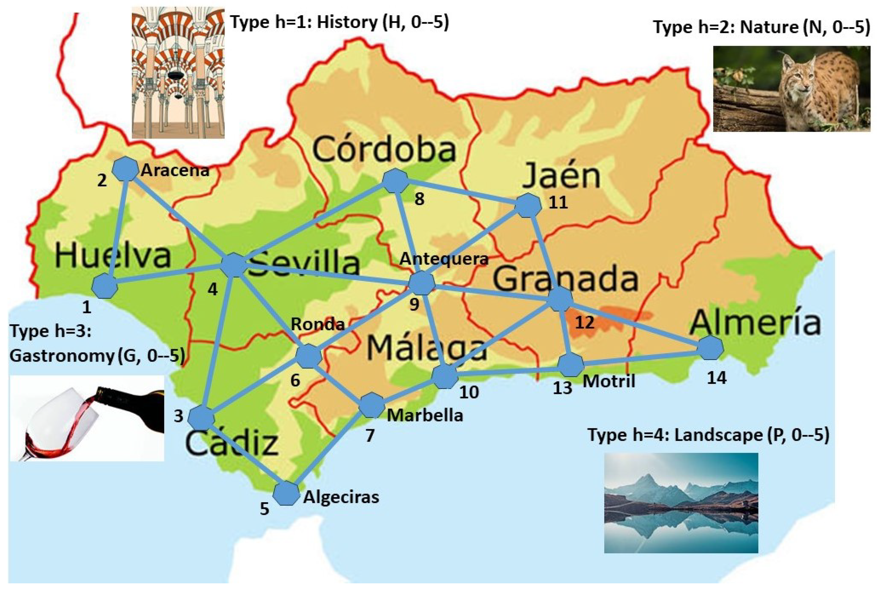
Let us suppose that the benefit to the traveler can be achieved when each arc is traversed. Let us consider that the geographical context considered can offer four types of attractive experiences for the traveler: historical elements (H), natural sites (N), gastronomic specialties (G) and landscape singularities (P). Let us also assume that each arc of the network can provide the traveler with a benefit of variable intensity, which has been normalized for the four types considered, by establishing a common scale, between the minimum value of 0 and the maximum value of 5.
The network used for this computational experience (see Figure 2) is inspired by the network of road connections with the highest capacity between the main towns in Andalusia.
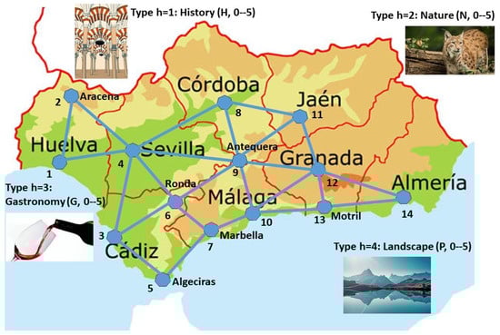
Figure 2.
Map of various route itineraries in Andalusia.
Figure 3 represents a graph of 24 feasible connections (in blue) between the 14 nodes. To simplify the complexity of the example, the connections are assumed to be undirected and the same travel time is required to travel through any of them. Thus, the limitation of the visit time can be associated with the total number of edges visited. Let us suppose that the maximum value of edges allowed for a feasible route is 6.
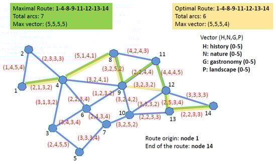
Figure 3.
Routes of maximum profit.
Additionally, each edge of the graph in Figure 3 is characterized by a vector (H,N,G,P) that, through values within the interval [0, 5], evaluates the interest of visiting such edge from the perspectives of its historical attraction, natural wealth, gastronomic importance and landscape value, respectively. The possible additional profits that can be achieved as a consequence of visiting the nodes are assumed to have already been accumulated in their respective edges, as indicated in the previous section.
Suppose that a traveler visits Andalusia (Spain), using a route that begins at node 1 (Huelva) and ends at node 14 (Almería), and wants to visit as many scenarios as possible in order to maximize enjoyment during their journey to various attractions associated with the route through the edges of the network (historical elements, natural sites, gastronomic specialties and singularities of the landscape). There is, as indicated above, the restriction that the total trip distance does not exceed 6 unit edges.
Logically, the ideal itinerary for the traveler should be oriented towards those edges where the maximum profit value could be achieved. Remember the benefits in the four types considered are normalized and scaled with numerical values between 0 and 5.
The execution of the proposed algorithm generates the following sets of arcs in Step 2:
(arcs where the maximum benefit value for type 1 is reached);
(arcs where the maximum benefit value for type 2 is reached);
(arcs where the maximum benefit value is reached for type 3);
(arcs where the maximum benefit value is reached for type 4).
By means of Step 3 of the proposed algorithm, the set is built.
Next, Step 4.(c) determines .
Through Step 4.(e).i., set is updated and the set of arcs is modified, thereby reconstructing the set of nodes .
In the following loop, the following results are obtained: , (step 4.(c)), (step 4.(e).i.), etc.
Figure 3 presents, in green, the route of maximum profit that can be achieved by applying the algorithm. Since this heuristic imposes no limitations on the total length of the path, the resulting itinerary exceeds the allowed length (six arcs at maximum). Such optimal route between nodes 1 and 14, where all the arcs are traveled with maximum benefit, is the sequence 1-2-4-8-11-12-13-14 (seven arcs, profit vector: ).
Given that the set of arcs where the maximum profit value is reached for type 3 (i.e., ) is widely represented, a new run of the algorithm could be carried out using a lower diversity of options for this set in Step 2 of the algorithm. For example, if arc were removed (i.e., ), the optimal path between nodes 1 and 14, where all the arcs are covered with maximum profit, would be the sequence 1-4-8-9-11-12-13-14.
Again, we would have obtained a solution of maximum benefit, but with an infeasible number of arcs in the total path (seven arcs; benefit vector (5,5,5,5); not feasible, again).
A new run of the algorithm can now be performed using an additional reduction on the same set. For example, eliminating the arc (8,9), considering that the set of arcs where the maximum benefit value for type 3 is reached is .
In this case, the optimal path between nodes 1 and 14 would be the sequence 1-4-8-11-12-13-14 (six arcs; profit vector (); feasible path!). See the yellow path in Figure 3.
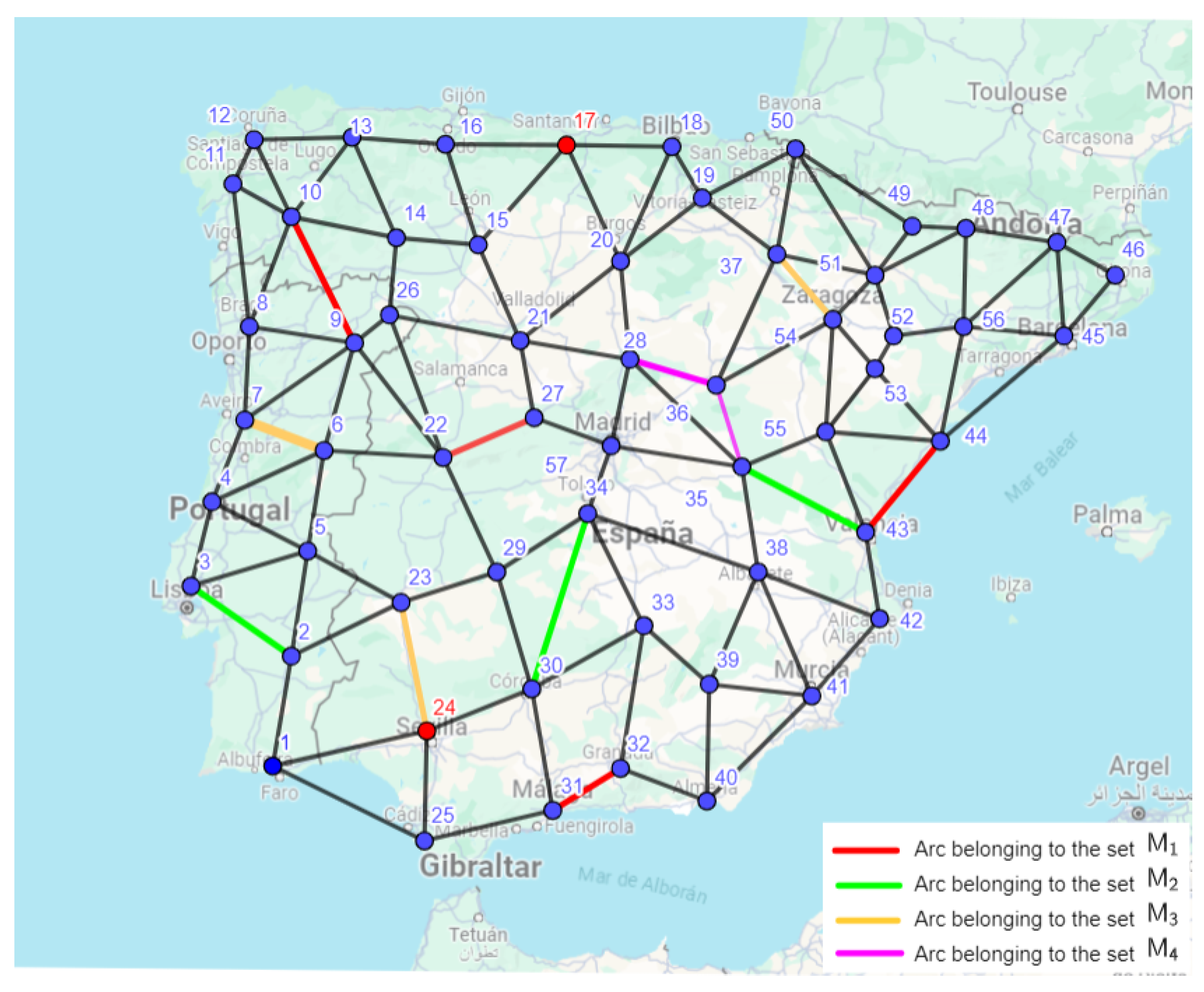
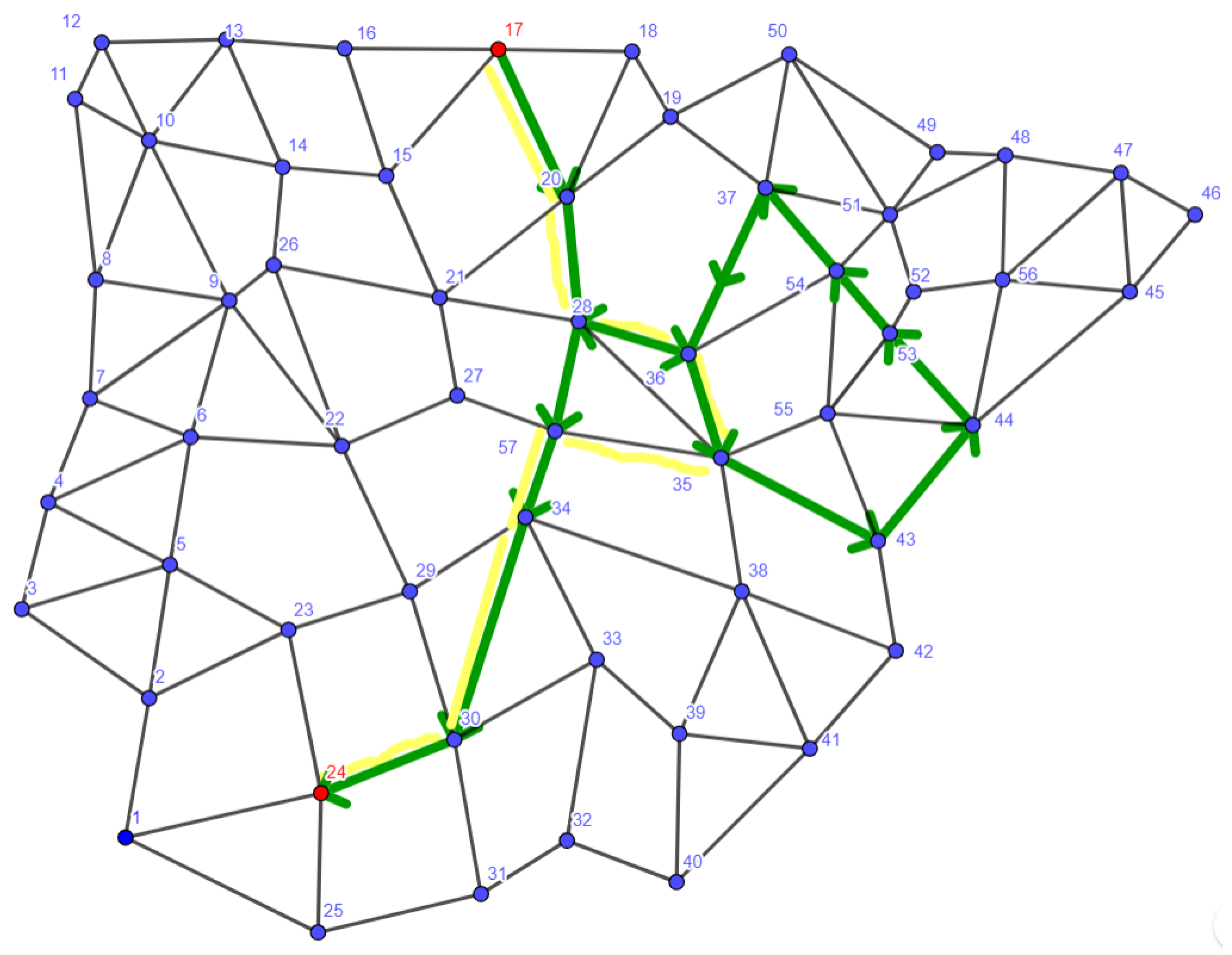
The algorithm also works for larger networks, such as that presented in Figure 4 inspired by the Iberian Peninsula. We have 57 nodes and 115 arcs, which we also consider undirected.
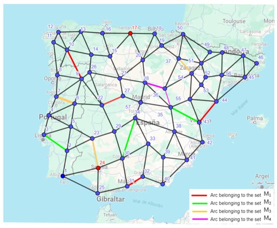
Figure 4.
Map of various itinerary routes in the Iberian Peninsula.
We consider the same tourist attractions with the same scale between 0 and 5. Let us assume that the maximum value of edges allowed for a feasible route is 8. Suppose a traveler visits the Iberian Peninsula, using a route that starts at node 17 (Santander) and ends at node 24 (Sevilla). The execution of the proposed algorithm generates in Step 2 the following sets of arcs (coloured in Figure 4):
(arcs where the maximum benefit value for type 1 is reached);
(arcs where the maximum benefit value for type 2 is reached);
(arcs where the maximum benefit value is reached for type 3);
(arcs where the maximum benefit value is reached for type 4).
Through Step 3 of the proposed algorithm, the set is built.
Next, Step 4. (c) determines .
Through Step 4. (f), set is updated, thereby reconstructing the set of nodes
In the following loop, the following results are obtained: (step 4.(c)), (step 4.(e).i.), etc.
Figure 5 presents, in green, the route of maximum profit that can be achieved by applying the algorithm. Since this heuristic imposes no limitations on the total length of the path, the resulting itinerary exceeds the allowed length (eight arcs at maximum). Such an optimal route between nodes 17 and 24, where all the arcs are traveled with maximum benefit, is the sequence 17-20-28-36-35-43-44-53-54-37-36-28-57-34-30-24 (fifteen arcs, profit vector: (5,5,5,5)).
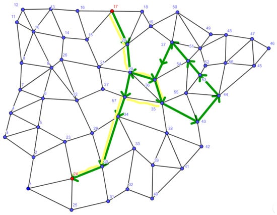
Figure 5.
Routes of maximum profit. Green route is the algorithm solution with original case. Yellow route is the algorithm solution with a modification of sets.
A new use of the algorithm could be carried out by eliminating those arcs m that belong to some and that are not feasible as part of the solution since to reach them from the origin and reach the destination from them with the shortest path, a route would have to be traveled whose length exceeds the maximum length. In this way, the arcs would be eliminated. Thus, the optimal route obtained would be the one corresponding to the sequence 17-20-28-36-35-57-34-30-24 (eight arcs; profit vector (); feasible path).
Wang et al. (2021) [45] used a two-part algorithm to solve the driver preference-based route planning (DPRP) problem, which consists of a first phase to eliminate those nodes and edges from the network that, if included in the chosen route, would exceed a threshold distance. The second phase of the algorithm is based on the concept of depth-first search traversal. It monitors the distance when accessing a route. Once it finds that the distance exceeds the threshold, it stops visiting the next point and cuts off the routes to be generated. However, they did not provide an algorithm to return the routes that best fit the driver’s preferences. These algorithms could also be used to reduce the size of the network in the TTDP scenario.
4. Conclusions and Future Work
In this study, the design of routes that offer travelers the acquisition of new knowledge is analyzed, within a high degree of diversity, running through arcs associated with different levels of profit according to the characteristics of each arc.
Since the benefit perceived by the visitor may be dependent on the time in which the route through each arch begins (due to, for example, natural light conditions, climate, tides, etc.), the possibility of duplicating routes and introducing waiting times in the nodes were taken into account in the discussion.
A mathematical optimization model, which could be defined as a Generalized Arc Orientation Problem (GAOP), has been formulated and, additionally, a heuristic algorithm was provided to solve the problem. The feasibility of the solutions can be affected by time limitations established to travel a given route. This consideration was commented on in the computational experience, providing a redefinition strategy in the input parameters that could alleviate such feasibility problems. The algorithm is applicable to different scales of transportation networks, from regional to national or continental networks. It can be adapted to plan ecotourism routes across a variety of geographic contexts and provide optimal solutions in each case.
In the article, Variance and Entropy were proposed as potential measures to assess the diversity of the identified eco-routes. It would be necessary to verify the effectiveness of these proposals; specifically, entropy has already been used to measure urban diversity [46], but it would be necessary to study whether it is also valid for measuring route diversity. This underscores the need for future research to explore the evaluation of the suggested measures and their applicability in accurately capturing diversity in the eco-routes.
Many natural spaces have restrictions on the types of vehicles that can circulate inside them. For future work, an interesting research direction would be to explore the adaptation of our developed model to the imperative use of electric vehicles with capacity constraints [47,48], where the limited number of charging stations and limited cruising range of electric vehicles must be considered during the design phase of the ecotourism routes.
Future research may also necessitate an investigation of the computational experience in determining the best option when the algorithm provides a solution with a length greater than the maximum. The option taken has been to remove edges from the most represented sets or edges that are unsuitable for helping reach the final solution; however, it would be interesting to incorporate that restriction into the algorithm or study which edges are best to remove.
Author Contributions
Conceptualization, R.P.-d.-l.-C. and F.A.O.; methodology, R.P.-d.-l.-C. and F.A.O.; writing—original draft, F.A.O.; writing—review & editing, R.P.-d.-l.-C. and F.A.O.; project administration, F.A.O. All authors have read and agreed to the published version of the manuscript.
Funding
This work was in part supported by the Proyecto I+D+i Junta de Andalucía (Spain)/FEDER under grant US-1381656.
Data Availability Statement
The data presented in this study are available on request from the corresponding author.
Acknowledgments
The authors are grateful for the financial support.
Conflicts of Interest
The authors declare no conflicts of interest.
References
- Vansteenwegen, P.; Van Oudheusden, D. The mobile tourist guide: An OR opportunity. OR Insight 2007, 20, 21–27. [Google Scholar] [CrossRef]
- Kellerer, H.; Pferschy, U.; Pisinger, D. Knapsack Problems; Springer: Berlin, Germany, 2004. [Google Scholar]
- Tsiligirides, T. Heuristic methods applied to orienteering. J. Oper. Res. Soc. 1984, 35, 797–809. [Google Scholar] [CrossRef]
- Chao, I.-M.; Golden, B.L.; Wasil, E.A. The team orienteering problem. Eur. J. Oper. Res. 1996, 88, 464–474. [Google Scholar] [CrossRef]
- Vansteenwegen, P.; Souffriau, W.; Oudheusden, D. The orienteering problem: A survey. Eur. J. Oper. Res. 2011, 209, 1–10. [Google Scholar] [CrossRef]
- Ruiz-Meza, J.; Montoya-Torres, J.R. A systematic literature review for the tourist trip design problem: Extensions, solution techniques and future research lines. Oper. Res. Perspect. 2022, 9, 100228. [Google Scholar] [CrossRef]
- Gunawan, A.; Lau, H.C.; Vansteenwegen, P. Orienteering problem: A survey of recent variants, solution approaches and applications. EJOR 2016, 255, 315–332. [Google Scholar] [CrossRef]
- Gavalas, D.; Konstantopoulos, C.; Mastakas, K.; Pantziou, G. A survey on algorithmic approaches for solving tourist trip design problems. J. Heuristics 2014, 20, 291–328. [Google Scholar] [CrossRef]
- Erdogan, G.; Laporte, G. The orienteering problem with variable profits. Networks 2013, 61, 104–116. [Google Scholar] [CrossRef]
- Afsar, H.M.; Labadie, N. Team orienteering problem with decreasing prof- its. Electron. Notes Discret. Math. 2013, 41, 285–293. [Google Scholar] [CrossRef]
- Vu, D.M.; Kergosien, Y.; Mendoza, J.E.; Desport, P. Branch-and-check approaches for the tourist trip design problem with rich constraints. Comput. Oper. Res. 2022, 138, 105566. [Google Scholar] [CrossRef]
- Porras, C.; Pérez-Cañedo, B.; Pelta, D.A.; Verdegay, J.L. A Critical Analysis of a Tourist Trip Design Problem with Time-Dependent Recommendation Factors and Waiting Times. Electronics 2022, 11, 357. [Google Scholar] [CrossRef]
- Gao, W.; Zhang, Q.; Lu, Z.; Wu, D.; Du, X. Modelling and application of fuzzy adaptive minimum spanning tree in tourism agglomeration area division. Knowl.-Based Syst. 2018, 143, 317–326. [Google Scholar] [CrossRef]
- Damos, M.A.; Zhu, J.; Li, W.; Hassan, A.; Khalifa, E. A Novel Urban Tourism Path Planning Approach Based on a Multiobjective Genetic Algorithm. ISPRS Int. J. Geo-Inf. 2021, 10, 530. [Google Scholar] [CrossRef]
- Suanpang, P.; Jamjuntr, P.; Jermsittiparsert, K.; Kaewyong, P. Tourism Service Scheduling in Smart City Based on Hybrid Genetic Algorithm Simulated Annealing Algorithm. Sustainability 2022, 14, 16293. [Google Scholar] [CrossRef]
- Souffriau, W.; Vansteenwegen, P.; Vertommen, J.; Vanden Berghe, G.; Van Oudheusden, D. A Personalized tourist trip design algorithm for mobile tourist guides. Appl. Artif. Intell. 2008, 22, 964–985. [Google Scholar] [CrossRef]
- Rodriguez, B.; Molina, J.; Perez, F.; Caballero, R. Interactive design of personalised tourism routes. Tour. Manag. 2012, 33, 926–940. [Google Scholar] [CrossRef]
- Souffriau, W.; Vansteenwegen, P.; Vanden Berghe, G.; Van Oudheusden, D. The planning of cycle trips in the province of East Flanders. Omega 2011, 39, 209–213. [Google Scholar] [CrossRef]
- Barrena, E.; Laporte, G.; Ortega, F.A.; Pozo, M.A. Planning Ecotourism Routes in Nature Parks; SEMA SIMAI Springer Series 8; Ortegón Gallego, F., Redondo Neble, M., Rodríguez Galván, J., Eds.; Trends in Differential Equations and Applications; Springer: Cham, Switzerland, 2016. [Google Scholar] [CrossRef]
- Ramesh, R.; Yong-Seok, Y.; Karwan, M.H. An optimal algorithm for the orienteering problem. ORSA J. Comput. 1992, 4, 155–165. [Google Scholar] [CrossRef]
- Vansteenwegen, P.; Gunawan, A. Orienteering Problems: Models and Algorithms for Vehicle Routing Problems with Profits; Springer: Cham, Switzerland, 2019. [Google Scholar]
- Hua, Q.; Zhang, Z.; Baldacci, R.; Tarantilis, C.D.; Zachariadis, E. The bus sightseeing problem. Intl. Trans. Oper. Res. 2023, 30, 4026–4060. [Google Scholar] [CrossRef]
- Deitch, R.; Ladany, S.P. The one-period bus touring problem: Solved by an effective heuristic for the orienteering tour problem and improvement algorithm. Eur. J. Oper. Res. 2000, 127, 69–77. [Google Scholar] [CrossRef]
- Feillet, D.; Dejax, P.; Gendreau, M. The profitable arc tour problem: Solution with a branch-and-price algorithm. Transp. Sci. 2005, 39, 539–552. [Google Scholar] [CrossRef]
- Zheng, Y.-T.; Yan, S.; Zha, Z.-J.; Li, Y.; Zhou, X.; Chua, T.-S.; Jain, R. Gpsview: A scenic driving route planner. ACM TOMCCAP 2013, 9, 1–18. [Google Scholar] [CrossRef]
- Skoumas, G.; Schmid, K.A.; Gregor Jossé, A.Z.; Nascimento, M.A.; Renz, M.; Pfoser, D. Towards knowledge-enriched path computation. In SIGSPATIAL ’14: Proceedings of the 22nd ACM SIGSPATIAL International Conference on Advances in Geographic Information Systems, Dallas, TX, USA, 4–7 November 2014; Association for Computing Machinery: New York, NY, USA, 2014; pp. 485–488. [Google Scholar]
- Quercia, D.; Schifanella, R.; Aiello, L.M. The shortest path to happiness: Recommending beautiful, quiet, and happy routes in the city. In HT ’14: Proceedings of the 25th ACM Conference on Hypertext and Social Media, Santiago, Chile, 1–4 September 2014; Association for Computing Machinery: New York, NY, USA, 2014; pp. 116–125. [Google Scholar]
- Ning, Z.; Sun, S.; Zhou, M.; Hu, X.; Wang, X.; Guo, L.; Hu, B.; Kwok, R.Y.K. Online Scheduling and Route Planning for Shared Buses in Urban Traffic Networks. IEEE Trans. Intell. Transp. Syst. 2022, 23, 3430–3444. [Google Scholar] [CrossRef]
- Corley, H.W.; Moon, I.D. Shortest paths in networks with vector weights. J. Optim. Theory Appl. 1985, 46, 79–86. [Google Scholar] [CrossRef]
- Skriver, A.J.V.; Andersen, K.A. A label correcting approach for solving bicriterion shortest path problems. Comput. Oper. Res. 2000, 27, 507–524. [Google Scholar] [CrossRef]
- Zheng, X.Y.; Han, B.T.; Ni, Z. Tourism route recommendation based on a multi-objective evolutionary algorithm using two-stage decomposition and Pareto layering. IEEE/CAA J. Autom. Sin. 2023, 10, 486–500. [Google Scholar] [CrossRef]
- Fox, B.L. Calculating Kth shortest paths. Infor Inform. Syst. Operat. Res. 1973, 11, 66–70. [Google Scholar]
- Eppstein, D. Finding the k shortest paths. SIAM J. Comput. 1998, 28, 652–673. [Google Scholar] [CrossRef]
- Raith, A.; Ehrgott, M. A comparison of solution strategies for biobjective shortest path problems. Comput. Oper. Res. 2009, 36, 1299–1331. [Google Scholar] [CrossRef]
- Pugliese, L.D.P.; Guerriero, F. A reference point approach for the resource constrained shortest path problems. Transport. Sci. 2013, 47, 131–294. [Google Scholar] [CrossRef]
- Srinivasan, K.K.; Prakash, A.A.; Seshadri, R. Finding most reliable paths on networks with correlated and shifted log-normal travel times. Transp. Res. Part B 2014, 66, 110–128. [Google Scholar] [CrossRef]
- Vanhove, S.; Fack, V. An effective heuristic for computing many shortest path alternatives in road networks. Int. J. Geograph. Inform. Sci. 2012, 26, 1031–1050. [Google Scholar] [CrossRef]
- Lindberg, K.; Hawkins, D.E. Ecotourism: A Guide for Planners and Managers; Ecotourism Society: North Bennington, VT, USA, 1993; Volume 1. [Google Scholar]
- Mathieson, A.; Wall, G. Tourism: Economic, Physical and Social Impacts; Longman Group: Essex, UK, 1982. [Google Scholar]
- Orams, M.B. Towards a more desirable form of ecotourism. Tour. Manag. 1995, 16, 3–8. [Google Scholar] [CrossRef]
- Buckley, R. Environmental Impact of Ecotourism; CAB International: Oxfordshire, UK, 2008. [Google Scholar]
- Dijkstra, E.W. A note on two problems in connection with graphs. Numer. Math. 1959, 1, 269–271. [Google Scholar] [CrossRef]
- Kelley, W.J. National Scenic Byways: Diversity Contributes to Success. Transp. Res. Rec. 2004, 1880, 174–180. [Google Scholar] [CrossRef]
- Ortega, F.A.; Marseglia, G.; Mesa, J.A.; Piedra-de-la-Cuadra, R. Algorithm for planning faster routes in urban networks with time-dependent arcs and the possibility of introducing waiting periods at nodes. WIT Trans. Built Environ. 2022, 212, 25–36. [Google Scholar]
- Wang, R.; Zhou, M.; Gao, K.; Alabdulwahab, A.; Rawa, M.J. Personalized route planning system based on driver preference. Sensors 2021, 22, 11. [Google Scholar] [CrossRef]
- Ortega, F.A.; Piedra-de-la-Cuadra, R.; Ventura, S. Applying an entropic analysis to locate rapid transit lines in sprawled cities. Int. J. Sustain. Dev. Plan. 2018, 13, 626–637. [Google Scholar] [CrossRef]
- Chen, Y.; Xue, J.; Zhou, Y.; Wu, Q. An Efficient Threshold Acceptance-Based Multi-Layer Search Algorithm for Capacitated Electric Vehicle Routing Problem. IEEE Trans. Intell. Transp. Syst. 2024, 1–13. [Google Scholar] [CrossRef]
- Piedra-de-la-Cuadra, R.; Ortega, F.A. Bilevel optimization for the deployment of refuelling stations for electric vehicles on road networks. Comput. Oper. Res. 2024, 162, 106460. [Google Scholar] [CrossRef]

Disclaimer/Publisher’s Note: The statements, opinions and data contained in all publications are solely those of the individual author(s) and contributor(s) and not of MDPI and/or the editor(s). MDPI and/or the editor(s) disclaim responsibility for any injury to people or property resulting from any ideas, methods, instructions or products referred to in the content. |
© 2024 by the authors. Licensee MDPI, Basel, Switzerland. This article is an open access article distributed under the terms and conditions of the Creative Commons Attribution (CC BY) license (https://creativecommons.org/licenses/by/4.0/).