Article

Design and Real-Time Implementation of a Cascaded Model Predictive Control Architecture for Unmanned Aerial Vehicles

by
Patricio Borbolla-Burillo
1,
David Sotelo
1,*,
Michael Frye
2,
Luis E. Garza-Castañón
1,
Luis Juárez-Moreno
1 and
Carlos Sotelo
1
1
Tecnologico de Monterrey, School of Engineering and Sciences, Ave. Eugenio Garza Sada 2501, Monterrey 64849, Mexico
2
Department of Engineering, University of the Incarnate Word, San Antonio, TX 78209, USA
*
Author to whom correspondence should be addressed.
Mathematics 2024, 12(5), 739; https://doi.org/10.3390/math12050739
Submission received: 17 December 2023 / Revised: 1 February 2024 / Accepted: 12 February 2024 / Published: 29 February 2024
(This article belongs to the Special Issue Dynamics and Control Theory with Applications)

Abstract

:
Modeling and control are challenging in unmanned aerial vehicles, especially in quadrotors where there exists high coupling between the position and the orientation dynamics. In simulations, conventional control strategies such as the use of a proportional–integral–derivative (PID) controller under different configurations are typically employed due to their simplicity and ease of design. However, linear assumptions have to be made, which turns into poor performance for practical applications on unmanned aerial vehicles (UAVs). This paper designs and implements a hierarchical cascaded model predictive control (MPC) for three-dimensional trajectory tracking using a quadrotor platform. The overall system consists of two stages: the mission server and the commander stabilizer. Different from existing works, the heavy computational burden is managed by decomposing the overall MPC strategy into two different schemes. The first scheme controls the translational displacements while the second scheme regulates the rotational movements of the quadrotor. For validation, the performance of the proposed controller is compared against that of a proportional–integral–velocity (PIV) controller taken from the literature. Here, real-world experiments for tracking helicoidal and lemniscate trajectories are implemented, while for regulation, an extreme wind disturbance is applied. The experimental results show that the proposed controller outperforms the PIV controller, presenting less signal effort fluctuations, especially in terms of rejecting external wind disturbances.

1. Introduction

In recent years, the use of UAV technology has notably increased. Quadrotors are preferred over other UAVs because of their versatility and their stable dynamics [1]. For this reason, they are used in aerial surveillance, shipping, emergency situations, entertainment shows, and agriculture monitoring, among other areas. These applications require the quadrotors to be fast, agile, and lightweight in order to be capable of following precise trajectories in the presence of external disturbances.
To meet these requirements, some control strategies have been developed [2,3,4,5,6,7]. First, the well-known PID controller, which can handle both linear and nonlinear systems, can achieve zero steady-state errors with a simple-to-understand tuning principle [2]. A linear–quadratic regulator (LQR) control can be easily implemented and can handle MIMO systems [3]. Feedback linearization (FL) provides the capacity to linearize a model with a model inversion procedure instead of making linearization assumptions [4]. Even though these control strategies can achieve adequate reference response, they are not robust and some of them even lack the ability to achieve zero steady-state errors [3,4].
MPC is one control strategy that is useful in handling multivariable processes. This method consists of an optimal control technique that calculates the necessary inputs of a model to minimize its cost function, which represents its system dynamics using its constraints over a limited time horizon [8]. Therefore, MPC is a robust control technique capable of controlling complex nonlinear systems while meeting the system constraints and ensuring safe operation [9]. However, the application of large-scale MPC in real-time has its own challenges, mainly due to its reliability, large computational overhead, and the complexity of its software implementation [10]. A literature survey presented recent real-time applications in which the MPC strategy was used to address these concerns [10,11,12,13,14,15,16,17,18]. For these reasons, the control of quadrotors using MPC has become feasible in more sophisticated applications as research of their control algorithms advances.
A variety of linear and nonlinear MPCs have been developed to improve control performance in quadrotors [19,20,21,22,23,24,25,26]. In [19], a compound control technique that consists of two different control strategies was described. They used both an integral sliding mode control to reject matched disturbances and an MPC to treat the remaining disturbances for successful trajectory tracking of a quadrotor. However, one of the main problems in MPC is the large computational capacity required. Therefore, in [20], the input sequence of an MPC was approximated with the Laguerre function, decreasing the computational burden and improving the inner loop performance of the quadrotor. Moreover, in [21], a simplified optimal control problem was proposed to reduce the computational burden of traditional MPCs so their proposed ‘bang-bang’ MPC could be applied to smaller and lighter quadrotors with less computational capacity. In [22], the authors employed a nonlinear MPC (NMPC) for the inner control loop of a quadrotor while maintaining the computation cost that is similar to a traditional NMPC.
On the other hand, system failures are always to be expected. For that reason, in [23], the authors developed an NMPC capable of stabilizing a drone during a rotor failure. Quadrotors should be able to adapt themselves to whatever model uncertainties they are subjected too. Therefore, in [24], the authors used a hybrid adaptive NMPC to learn the model uncertainties in real time. This control algorithm improved the quadrotor’s control robustness and reduced tracking error by 90% compared to a non-adaptive NMPC while keeping the computational overhead burden at a minimum. In [25], an NMPC scheme was proposed for obstacle avoidance in quadrotors; the authors applied a potential field function-based penalty term and a dynamical adjustment for the prediction horizon to cut down the heavy computational load. Similarly, in [26], an NMPC for obstacle avoidance was employed; in this case, the NMPC control was formulated in the special Euclidean group SE(3) for the quadrotor to operate in messy environments with a large number of obstacles. Simulations were performed using algebraic ellipsoids as obstacles.
Although tremendous effort has been dedicated to implementing MPC in unmanned systems [27], there still exist significant challenges in high-speed real-time applications. An MPC is designed based on the entire nonlinear dynamics model of a quadrotor UAV, which introduces several computational challenges [18,28], and its real-time applicability is reduced. To avoid this, linear control strategies have been implemented while considering the advantages of being relatively easy to understand and design [29]. The linearization procedure is carried out by first trimming the quadrotor at zero wind and then at hover [30]. Thus, it is sufficient to use a single linear time invariant (LTI) model for MPC [27,31]. In this paper, to address the drawbacks of the advanced control strategies in quadrotors mentioned in [14,32], the real-time implementation is addressed. Here, the computationally efficient control architecture for a multivariable system is obtained, which reduces the complexity of the system dynamics and improves its real-time performance [13,33]. The overall MPC strategy is decomposed into two different schemes [16,34]. The first scheme controls the translational displacements while the second scheme regulates the rotational movements of the quadrotor. This turns into a less computationally expensive scheme, which is suitable for real-time implementation. To validate the tracking performance of the proposed MPC architecture, it is compared to a PIV controller with three real-time scenarios: tracking helicoidal, tracking lemniscate, and aggressive regulator under extreme external disturbances. All tests were carried out with a QDrone 2 quadrotor from Quanser® [28,35].
This paper is organized as follows. Section 2 states the dynamic model of the QDrone 2 quadrotor UAV. Section 3 gives an overview of the MPC control technique. Section 4 details the overall system used for implementation, including the compared PIV control structure and the proposed MPC control scheme and its algorithm. Section 5 contains all the tuning and hardware parameters and presents the tracking and regulator scenarios. The implementation results illustrate the performance improvement of the proposed cascaded MPC control structure compared to a PIV controller. Finally, in Section 6, the paper summarizes the results and future work.

2. Kinematics

First, to model the quadrotor dynamics with the Newton–Euler formalism taken from the literature [36], it is necessary to consider two frames, the inertial frame ( o w x w y w z w ) and the quadrotor body frame ( o b x b y b z b ). These two reference frames are needed to define both the position and orientation of the quadrotor UAV (Figure 1). Considering that each propeller contributes individually to the movement of the whole system, the force generated by each propeller and the thrust produced by the quadrotor is defined by
f i = k ω i 2
T = 0 0 i = 1 4 f i
where k is the lift constant and ω is the angular velocity of the rotor. Therefore, as the four rotors are fixed pointing upwards, the total thrust generated will be on the z b axis. The total thrust is equivalent to the sum of the forces generated by the rotors.
In the inertial frame, the absolute position is defined by a linear position vector ξ with the coordinates x w , y w , z w , and an angular position vector η with the roll, pitch, and yaw angles, expressed as ϕ , θ , ψ , respectively.
ξ = x w y w z w T
η = ϕ θ ψ T
On the other hand, the body frame is defined by a linear position vector σ with x b , y b , z b coordinates, and an angular velocity vector γ with p , q , r .
σ = x b y b z b T
γ = p q r T
Both the inertial fixed frame and the body fixed frame linear-movement vectors are related by the transformation matrix R L taken from the Z Y X Tait–Bryan angles [37], where C and S denote cosine and sine functions, respectively.
R L = C ψ · C θ C ψ · S θ · S ϕ S ψ · C ϕ C ψ · S θ · C ϕ + S ψ · S ϕ S ψ · C θ S ψ · S θ · S ϕ + C ψ · C ϕ S ψ · S θ · C ϕ C ψ · S ϕ S θ C θ · S ϕ C θ · C ϕ
ξ = R L · σ
Similar to R L , there is also a rotational movement transformation matrix R R that relates the angular velocity vectors from the inertial and body fixed frames [37].
R R = 1 0 S θ 0 C ϕ C θ · S ϕ 0 S ϕ C θ · C ϕ
γ = R R · η ˙
The translational dynamical model of the quadrotor in the inertial fixed frame based on Newton’s second law of translational motion is
m · ξ ¨ = 0 0 m g k d L ξ ˙ + R L T
where T is the thrust vector, m is the mass of the quadrotor, k d L is the thrust drag coefficient, and g is the Earth’s gravity constant. On the other hand, the rotational dynamical model in the body fixed frame using Euler’s equation of rotational motion is the following:
I γ ˙ = τ γ × I γ μ k d R γ
τ = l r ( f 2 f 4 ) l p ( f 1 f 3 ) d ( ω 1 2 ω 2 2 + ω 3 2 ω 4 2 )
ω Γ = ω 1 ω 2 + ω 3 ω 4
μ = I R γ × 0 0 1 ω Γ
I = I x x 0 0 0 I y y 0 0 0 I z z
where μ is the gyroscopic moment vector [38]; k d R is the moment drag coefficient; I R is the gyroscopic inertia vector induced by the propellers; d is the drag coefficient; I is the diagonal matrix of inertia; ω Γ is the residual angular speed of the rotors; and l r and l p are the lengths between the quadrotor center of mass and the rotor that corresponds to the roll and pitch angle, respectively. Then, the complete nonlinear dynamical model of the quadrotor is based on the following equations:
x ¨ w = U 1 m C ψ · S θ · C ϕ + S ψ · S ϕ k d L x ˙ w m
y ¨ w = U 1 m S ψ · S θ · C ϕ C ψ · S ϕ k d L y ˙ w m
z ¨ w = U 1 m C θ · C ϕ g k d L z ˙ w m
p ˙ = U 2 I x x + I y y I z z I x x q r I R ω Γ I x x q k d R I x x p
q ˙ = U 3 I y y + I z z I x x I y y p r + I R ω Γ I y y p k d R I y y q
r ˙ = U 4 I z z + I x x I y y I z z p q k d R I z z r
Here, the quadrotor system consists of four input variables described in vector U
U = U 1 U 2 U 3 U 4 = k k k k 0 l r k 0 l r k l p k 0 l p k 0 d d d d ω 1 2 ω 2 2 ω 3 2 ω 4 2
where U 1 denotes the total thrust, U 2 and U 3 stand for the torques generated about ϕ and θ axes, respectively, and U 4 is the moment produced about the ψ axis. Thus, the choice of state vector is given as follows
X = x w y w z w x ˙ w y ˙ w z ˙ w ϕ θ ψ p q r T
Moreover, considering linear control techniques are widely used for UAV flight control [28,30,31,34,39], as they can ensure optimal performance when operating close to the equilibrium point [40,41], a linearization of the model under the following assumptions is carried out:
  • Standard quadrotor structure.
  • The structure is perfectly rigid.
  • The center of mass of the quadrotor coincides with the origin of the body frame.
  • Aerodynamics and other complex phenomena that are difficult to model are ignored.
  • The quadrotor is hovering.
Then, considering that the quadrotor is assumed to be in hover position [30], the following is true:
ϕ = θ = ψ 0 , ϕ ˙ = θ ˙ = ψ ˙ 0
I R 0 , k d L 0 , k d R 0
( ϕ ˙ , θ ˙ , ψ ˙ ) ( p , q , r )
U = U 1 U 2 U 3 U 4 = m g 0 0 0
Given that x ¨ w depends directly on θ and y ¨ w depends directly on ϕ , the input U 1 , Equation (28), is substituted in (17) and (18) [42]. Then, by performing small-angle approximations and eliminating the products of two terms near zero, the linearized dynamical model used for the proposed MPC is obtained:
x ¨ w = g θ
y ¨ w = g ϕ
z ¨ w = U 1 m g
ϕ ¨ = U 2 I x x
θ ¨ = U 3 I y y
ψ ¨ = U 4 I z z
The linearized dynamics in (29)–(34) are decoupled for state space representation. Each of them follows the state space structure Ax + Bu.The altitude controller (31) is rewritten as
z ˙ w z ¨ w = 0 1 0 0 z w z ˙ w + 0 1 m T + g
where m corresponds to the mass of the drone and
g = 0 g
For the x w y w position controller, (29) and (30) can be represented as
x ˙ w x ¨ w y ˙ w y ¨ w = 0 1 0 0 0 0 0 0 0 0 0 1 0 0 0 0 x w x ˙ w y w y ˙ w + 0 0 g 0 0 0 0 g θ d ϕ d
And the state space representation of the rotational dynamics, (32)–(34) can be rewritten as
ϕ ˙ ϕ ¨ θ ˙ θ ¨ ψ ˙ ψ ¨ = 0 1 0 0 0 0 0 0 0 0 0 0 0 0 0 1 0 0 0 0 0 0 0 0 0 0 0 0 0 1 0 0 0 0 0 0 ϕ ϕ ˙ θ θ ˙ ψ ψ ˙ + 0 0 0 1 I x x 0 0 0 0 0 0 1 I y y 0 0 0 0 0 0 1 I z z τ
The controllability of the linearized system is tested before the design of the controller. Here, the controllability matrix has full rank, which implies that the linear system is controllable. On the other hand, even though the system is unstable, linear controllers ensure system stability and optimal performance when operating close to the equilibrium point [40,41].

3. Control Strategy

In this section, MPCs are designed for translational and rotational dynamics. The translational subsystem considers two MPCs, one for altitude and the other for x w y w position; meanwhile, the rotational subsystem has an MPC for attitude. Hence, the control actions are obtained in each subsystem separately.
The MPC strategies for x w y w position and attitude are based on [43]. However, considering that z w axis depends on gravity constant g, the following LTI state space model is used to represent the altitude system dynamics:
x k + 1 = A x k + B u ( k ) + g
y k = C x ( k )
where the state vector is denoted as x R n , the input vector is u R n u , the output vector is y R n y , the state matrix is A R n × n , the input matrix is B R n × n u , the output matrix is C R n y × n , and the sampling time is expressed as k N . Furthermore, the projection matrix Π i ( n , N ) is defined as follows:
Π i ( n , N ) 0 n × n 0 n × n i 1 t e r m s I n × n 0 n × n 0 n × n N i t e r m s
where n stands for the vector length, N refers to the prediction horizon, and i is the term desired.
Then, the state predictions for the sampling time are
x k + 1 = A x k + B u k + g , x k + 2 = A 2 x k + AB u k + B u k + 1 + Ag + g , x k + i = A i x k + A i 1 B AB B u k u k + i 2 u k + i 1 + A i 1 B A I g g g , x k + i = A i x k + A i 1 B AB B Π 1 ( n u , N ) Π i 1 ( n u , N ) Π i ( n u , N ) u ˜ ( k ) + A i 1 A I g ˜ ,
x k + i = Φ i x k + Ψ i u ˜ k + Θ i g ˜ , i { 1 , , N }
where Φ i R n × n , Ψ i R n × ( N n u ) , and Θ i R n × ( N n ) stand for the N-step-ahead in LTI systems in a more compact manner [44]. Hence, the above equation can be reformulated in the following form:
x ˜ k = Φ x k + Ψ u ˜ k + Θ g ˜
where Φ = Φ 1 Φ 2 Φ N T , Ψ = Ψ 1 Ψ 2 Ψ N T , Θ = Θ 1 Θ 2 Θ N T ,   x ˜ k R N · n u stands for the whole state trajectory of x = x 1 x 2 x n T ; u ˜ k R N · n u contains the computed sequence of u = u 1 u 2 u n u T ; g ˜ R ( N · n ) contains the gravity vectors g = 0 g T ; and y ˜ k R N · n y is the output trajectory of y = y 1 y 2 y n y T . Then, depending on the prediction horizon N , x ˜ k , u ˜ k , and y ˜ k are expressed as
x ˜ k x ( k + 1 ) x ( k + 2 ) x ( k + N ) , u ˜ k u ( k ) u ( k + 1 ) u ( k + N 1 ) , y ˜ k y ( k + 1 ) y ( k + 2 ) y ( k + N ) .
Thus, given this formulation, any chain of inputs u ˜ k has its corresponding set of future states x ˜ k and outputs y ˜ k . Now, the state, input, and output vectors at an instant k + i can be obtained with
x k + i = Π i ( n , N ) · x ˜ k ,
u k + i 1 = Π i ( n , N ) · u ˜ k ,
y k + i = Π i ( n y , N ) · y ˜ k .
Now, considering that all linear stable systems are quadratically stable [28], the cost function J u ˜ | x k , w ˜ d k , u d to find the best possible set of actions in the prediction horizon [ k , k + N ] is presented [43]
J i = 1 N Π i ( n y , N ) · y ˜ Π i ( n y , N ) · w ˜ d Q 2 + i = 1 N Π i ( n u , N ) · u ˜ u d R 2
In the first term, the error between the output trajectory y ˜ k R N · n y and the reference w ˜ d ( k ) R N · n y is penalized by the positive definite matrix Q R n y × n y . Here, w ˜ d ( k ) contains the sequence of references w d = w 1 d w 2 d w n y d T , in which, depending on the prediction horizon N , w ˜ d ( k ) can be expressed as
w ˜ d k w d ( k + 1 ) w d ( k + 2 ) w d ( k + N )
Additionally, in the second term, the difference between the input vector u ˜ k and the desired input u d R n u is penalized by the positive definite weighting matrix R R n u × n u . Therefore, the minimization problem is solved to find the input vector u ˜ k ; however, only the first control input is implemented on the system. Then, the system moves to k + 1 to solve the minimization problem again for the new control action.
The above cost function is rewritten using notations (45) and (46):
J i = 1 N y ( k + i ) w d ( k + i ) Q 2 + i = 1 N Π i ( n u , N ) · u ˜ u d R 2
Hence, the general cost function implemented for the altitude controller in space state representation is as follows:
J i = 1 N C Φ i x k + C Ψ i u ˜ k + C Θ i g ˜ Π i ( n y , N ) w ˜ d ( k ) Q 2 + i = 1 N Π i ( n u , N ) · u ˜ u d R 2
Thus, the control law can be obtained by rewriting the performance index in a more compact form, as follows:
J 1 2 u ˜ T H u ˜ + F 1 x ( k ) + F 2 w ˜ d ( k ) + F 3 u d + F 4 T u ˜
where
H 2 i = 1 N Ψ i T C T Q C Ψ i + Π i n u , N T Q ( Π i ( n u , N ) )
F 1 2 i = 1 N Ψ i T C T Q C Φ i
F 2 2 i = 1 N Ψ i T C T Q Π i ( n y , N )
F 3 2 i = 1 N Π i ( n u , N ) T R
F 4 2 i = 1 N Ψ i T C T Q C Θ i g ˜
Then, from (50), the control law is obtained:
u ˜ o p t x k = H 1 F 1 x k + F 2 w ˜ d ( k ) + F 3 u d + F 4
When applying the first action of the control input chain u ˜ o p t x k , the MPC state feedback can be expressed as
K M P C ( x k ) = Π i n u , N · u ˜ o p t x k , w ˜ d k , u d
Moreover, the optimization problem below is addressed at every sample time instant; therefore, the measurements of the states and outputs of the system are updated constantly.
P x k : min u ˜ R N n u J u ˜ | x k , w ˜ d k , u d

4. Quadrotor Control Structure

The overall system structure shown in Figure 2 for this implementation consists of two stages: the mission server and the commander stabilizer. The mission server stage is equipped with an OptiTrack® Flex13 motion tracking system, providing the UAV location in real-time at 120 Hz to the main PC workstation. Here, as the communication between the server and the UAV is continuous, complex reference trajectories are sent by the user in real time. Therefore, the actual and desired coordinates serve as inputs to the commander stabilizer stage. The commander stabilizer corresponds to the main elements of the Quanser® QDrone 2 platform, such as the onboard PC, battery, and rotors. The onboard PC, NVIDIA Jetson Xavier NX SOM, contains the proposed control structure MPC, a control input PWM translator, and a battery drop compensator. Additionally, the quadrotor includes a 4S 14.8 V LiPo (3700 mAh) battery to actuate four motors with 6-inch propellers, each providing a maximum of 8.5 N lift force. Thus, the mission server and the commander stabilizer use QUARC™ 2023 SP2 software to generate real-time code directly from SIMULINK®.
Thus, based on Figure 2, the overall control process is described in detail:
  • The camera system provides the linear and yaw positions of the quadrotor, while the IMU of the quadrotor sends the angular status.
  • The trajectory generator commands the desired position in the inertial frame ( x w d , y w d , z w d ) . These will be the references for translational control.
  • The implemented cascaded control structures, PIV, and MPC receive the desired and actual position and rotational coordinates to compute U 1 , U 2 , U 3 , U 4 .
  • Once all the control actions are calculated, the transformation matrix provided by Quanser® is used to change the control inputs to pulse-width modulation (PWM).
    T m = 0.0489 0.4581 0.5566 5.1335 0.0489 0.4581 0.5566 5.1335 0.0489 0.4581 0.5566 5.1335 0.0489 0.4581 0.5566 5.1335
  • Most of the quadrotors in real-world implementations are powered by batteries [45]. Here, the reduction in power supply, named battery drainage, occurs gradually [46,47]. Therefore, the control performance of the drone is affected [48]. For this reason, we designed a compensation subsystem by measuring the altitude and battery voltage rate of change. Hence, a relationship between the PWM and the necessary battery level to reach hover position was obtained.
  • The rotors receive their compensated PWM control signal.

4.1. PIV Controller Design

The main difference between the PIV controller and the well-known PID controller comes from the definition of the error [49]. In the PID, only the position error e p is considered, whereas in the PIV, the position and velocity errors, e p and e v , are considered. Here, the velocity error is obtained not from the time derivative of the position error, but from calculating the difference between the desired velocity and the actual velocity of the quadrotor. Then, the compared PIV controller can be defined with the following equation:
P I V = K p e p + K i e i + K v e v
where e i stands for the position error integral with respect to time of e p , and K p , K i , K v represent the proportional, integrative, and velocity constants, respectively. Thus, Figure 3 shows the PIV control structure.
Hence, based on Figure 2 and Figure 3, the overall PIV control process is described in detail:
  • The position PIV controller obtains the desired x w d , y w d , z w d positions from the trajectory generator while the motion tracking system provides the actual x w , y w , z w position of the drone. Here, the thrust input U 1 and the angular reference ϕ d , θ d of the angular PIV are computed as follows:
    U 1 = k p z w e z w + k i z w 0 e z w k v z w z ˙ w
    ϕ d = k p y w e y w + k i y w 0 e y w k v y w y ˙ w
    θ d = k p x w e x w + k i x w 0 e x w k v x w x ˙ w
  • Then, the angular PIV receives the desired angular positions ( ϕ d , θ d , ψ d ) , the actual angular positions ( ϕ , θ , ψ ) , and the actual angular velocities ( ϕ ˙ , θ ˙ , ψ ˙ ) . These are processed to compute the reference angular velocities ( ϕ ˙ d , θ ˙ d , ψ ˙ d ) of the PIV velocities, which are saturated with a minimum and a maximum rate of −45° and 45°, respectively.
    ϕ ˙ d = k p ϕ e ϕ k v ϕ ϕ ˙
    θ ˙ d = k p θ e θ k v θ θ ˙
    ψ ˙ d = k p ψ e ψ k v ψ ψ ˙
  • The angular PIV velocity gathers the desired angular velocities ( ϕ ˙ d , θ ˙ d , ψ ˙ d ) , the actual angular velocities ( ϕ ˙ , θ ˙ , ψ ˙ ) , and the actual angular accelerations ( ϕ ¨ , θ ¨ , ψ ¨ ) . Then, it computes the optimal angular torques ( U 2 , U 3 , U 4 ) ; this is performed by considering the thrust input ( U 1 ) computed in step (a).
    U 2 = k p ϕ ˙ e ϕ ˙ k v ϕ ˙ ϕ ¨
    U 3 = k p θ ˙ e θ ˙ k v θ ˙ θ ¨
    U 4 = k p ψ ˙ e ψ ˙
The PIV controllers always stabilize with respect to the attitude commands’ set point. Here, the attitude torques are added to the output of the remaining PIV controllers to generate the generalized force.

4.2. MPC Controller Design

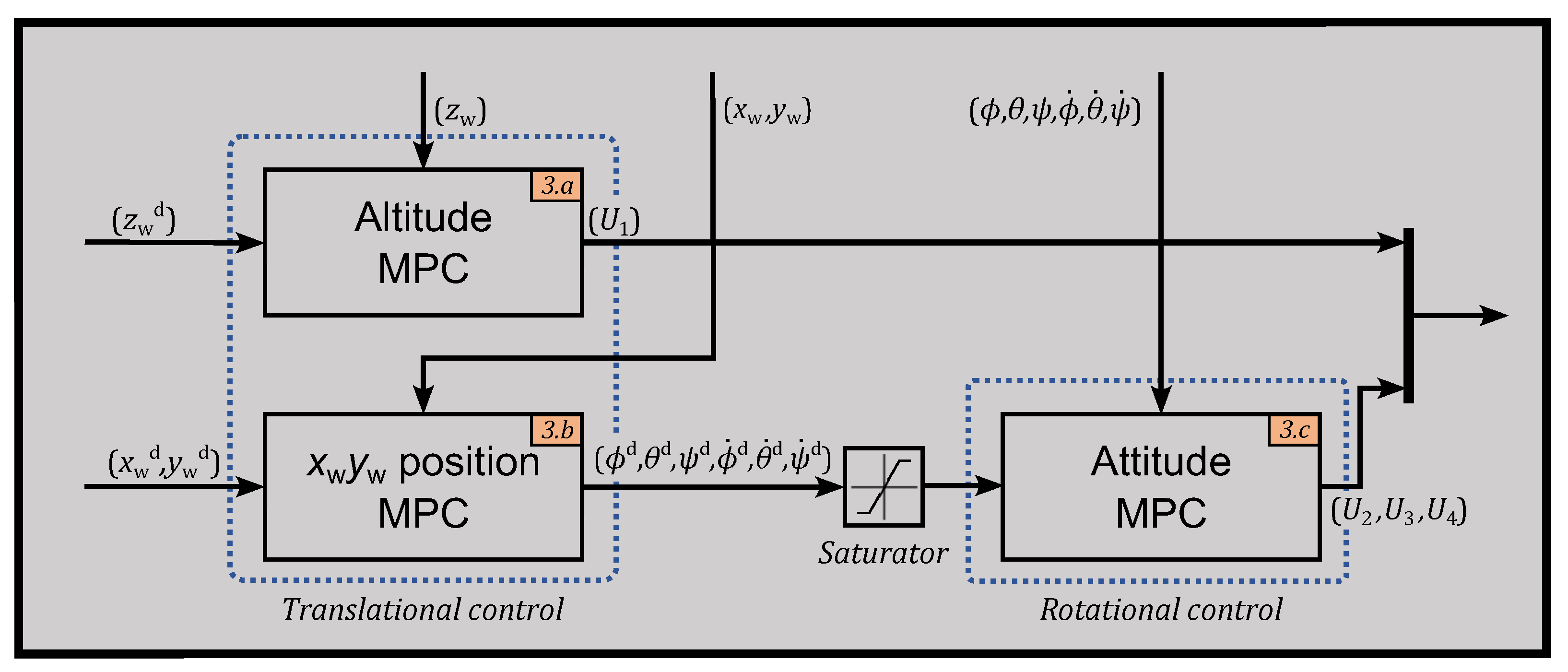
The proposed cascaded MPC translational and rotational structure is shown in Figure 4, which considers the dependency between the linear displacement and the rotation of the drone.
The translational control (outer loop) tracks the altitude while computing the thrust input ( U 1 ) , and the x w y w position, feeding the reference orientations to the rotational control. Then, the rotational control (inner loop) tracks the attitude, applying feasible torques ( U 2 , U 3 , U 4 ) to the quadrotor.
The proposed cascaded MPC used to fulfill the linear drone dynamics works as follows:
  • The altitude controller obtains the reference z w d from the trajectory generator while the motion tracking system provides the actual z w position of the drone. Here, the thrust input U 1 is computed.
  • On the other hand, x w and y w accelerations depend directly on the rotation of the drone. Thus, the dynamics are dependent, and the controllers must be related. This relation is described in the dynamical models (29), (30), where it is shown that the product between gravity and the respective angle gives a linear displacement. Then, the output of the x w y w MPC algorithm is saturated with a minimum and maximum of −45° and 45°, respectively, and the desired angles are sent to the attitude controller.
  • The attitude MPC receives the following: from the motion tracking system, the angular positions ( ϕ , θ , ψ ) and the angular velocities ( ϕ ˙ , θ ˙ , ψ ˙ ) ; and from the x w y w MPC algorithm, the saturated orientation references ( ϕ d , θ d , ψ d , ϕ ˙ d , θ ˙ d , ψ ˙ d ) . Then, the attitude MPC uses this information to obtain the optimal angular torques ( U 2 , U 3 , U 4 ) ; factoring into the calculations the thrust input ( U 1 ) computed in step (a).
Additionally, for the translational and rotational control described in detail in this section, each MPC controller works according to the following algorithm in Table 1.

5. Real-Time Implementation

5.1. Experimental Setup

In this section, flight experiments are carried out to validate the effectiveness of the proposed cascaded MPC strategy compared to the traditional PIV control scheme. Table 2 shows the quadrotor parameters of the QDrone 2 for the real-time implementation programmed using MATLAB® SIMULINK® [50].
The constant values for the PIV implementation are shown in Table 3 [28,35]. Here, the PIV controller parameters K p , K i , and K v are defined for the positions ( x w , y w , z w ) , the angular positions ( ϕ , θ , ψ ) , and the angular velocities ( ϕ ˙ , θ ˙ , ψ ˙ ) of the drone.
On the other hand, the tunning parameters for a desired closed loop performance of each MPC controller are presented in Table 4.

5.2. Experimental Results

To validate the performance of the proposed cascaded MPC controllers over the conventional PIV control structure, the following three scenarios are real-time implemented:
  • Scenario 1. Helicoidal trajectory;
  • Scenario 2. Lemniscate trajectory;
  • Scenario 3. Wind disturbance rejection.
Hence, to demonstrate the ability of a quadrotor in automatic flight mode, scenario 1 and scenario 2 are selected, considering that they are commonly used as a standard benchmark for tracking control [37]. Meanwhile, to test the performance of the quadrotor under external disturbances, scenario 3 is selected for regulatory control [51]. Therefore, the positions ( x w , y w , z w ) and the PWM signals in voltage of each rotor ( m 1 , m 2 , m 3 , m 4 ) based on the control inputs ( U 1 , U 2 , U 3 , U 4 ) must be plotted.

5.2.1. Scenario 1: Helicoidal Trajectory

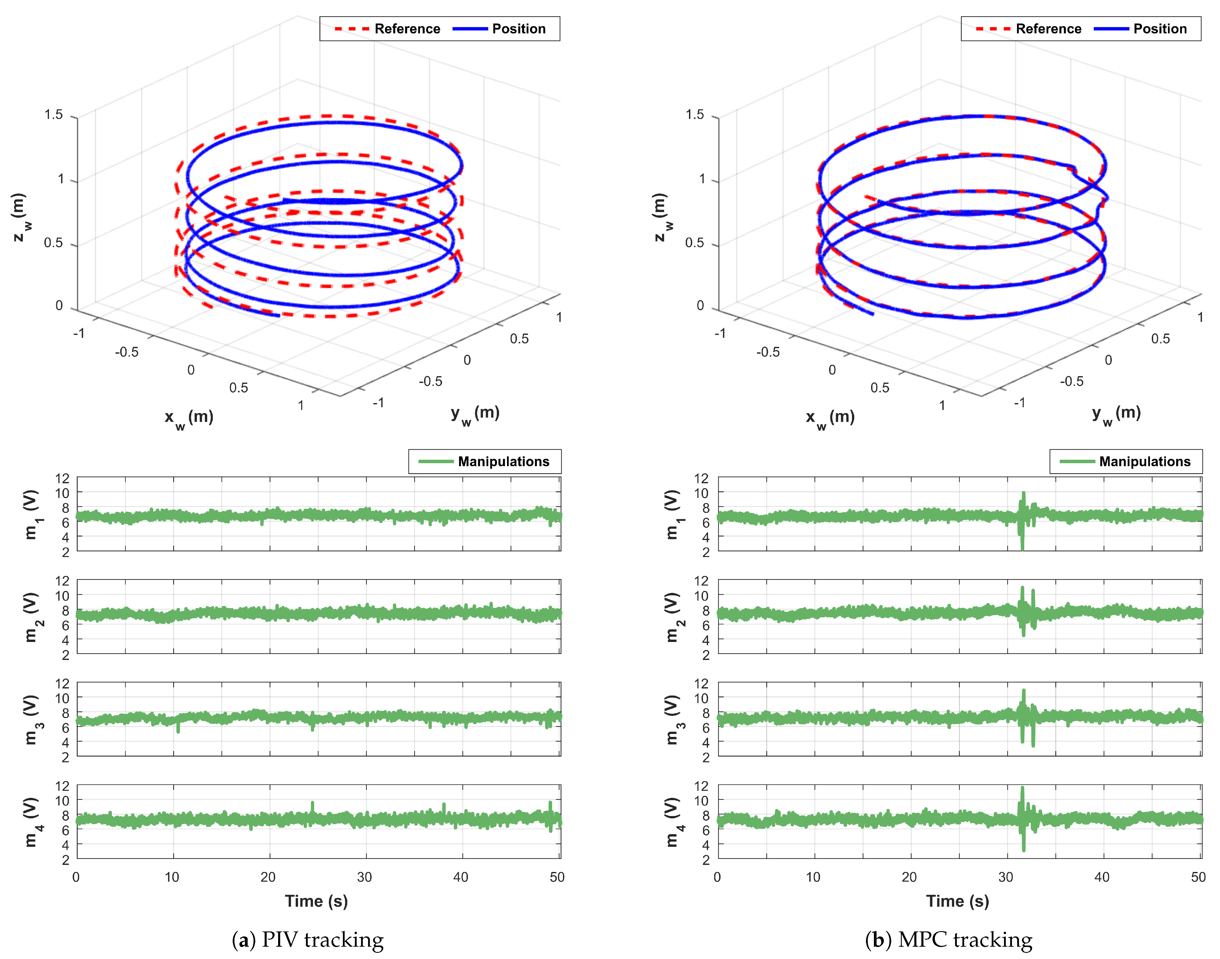
Regarding the first scenario, the helicoidal trajectory is given by Equation (66). Figure 5 shows the comparison between the proposed MPC controller performance with respect to PIV control structure.
x w d = sin 0.5 t y w d = cos 0.5 t z w d = 0.5 sin 0.05 t
Here, even though the quadrotor under the MPC control strategy had a communication error between the main PC workstation and the UAV at 35 s, the comparison indicates that the MPC does not present steady-state errors compared to the PIV control method.

5.2.2. Scenario 2: Lemniscate Trajectory

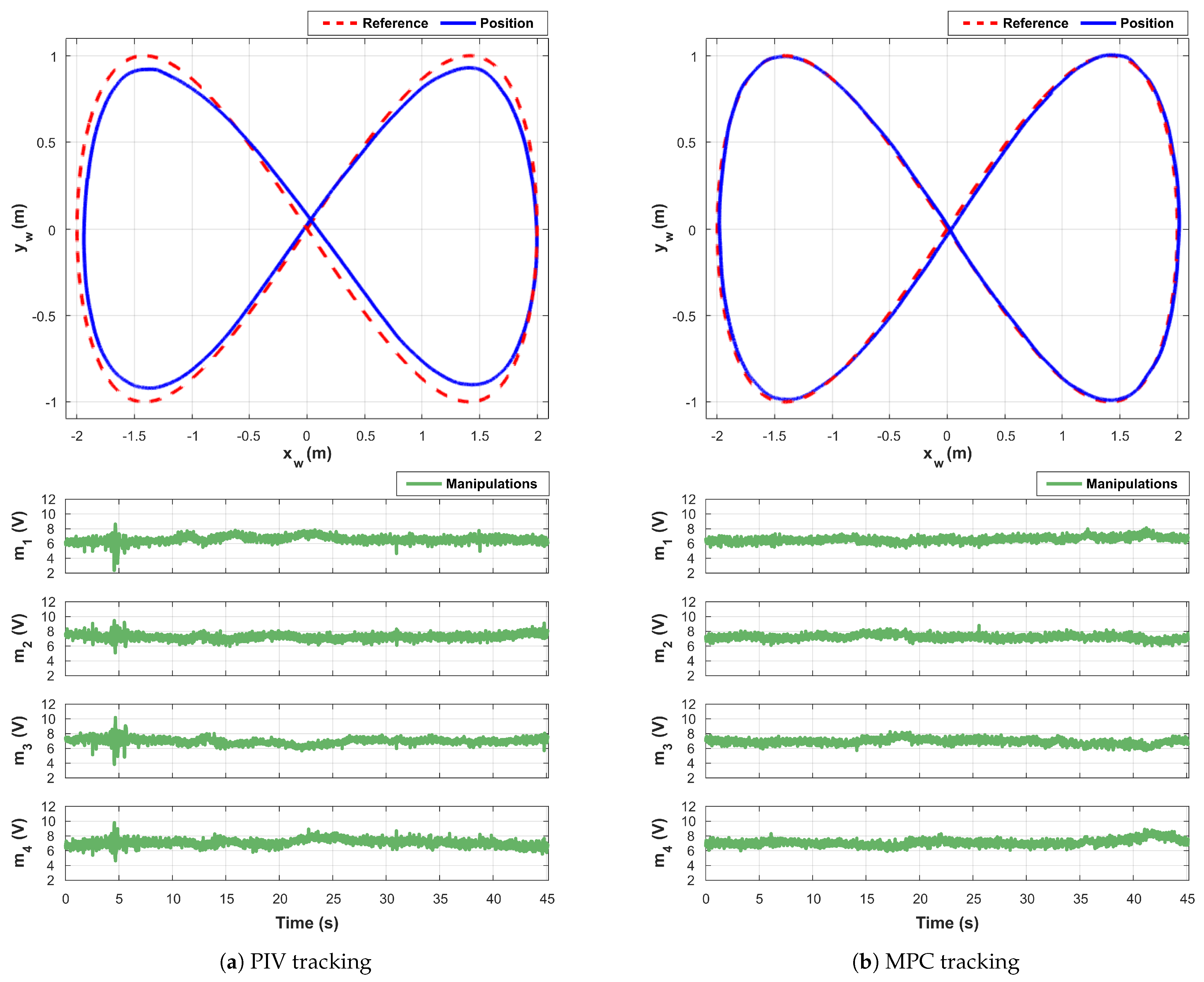
For the second scenario, a lemniscate trajectory is programmed in the main PC workstation based on the Equation (67). Figure 6 shows the comparison between the proposed MPC controller performance with respect to PIV control strategy.
x w d = 2 cos 1 45 t y w d = sin 2 45 t
Similarly to scenario 1, the tracking results for scenario 2 show that the PIV control presents steady-state errors.

5.2.3. Scenario 3: Disturbance Rejection

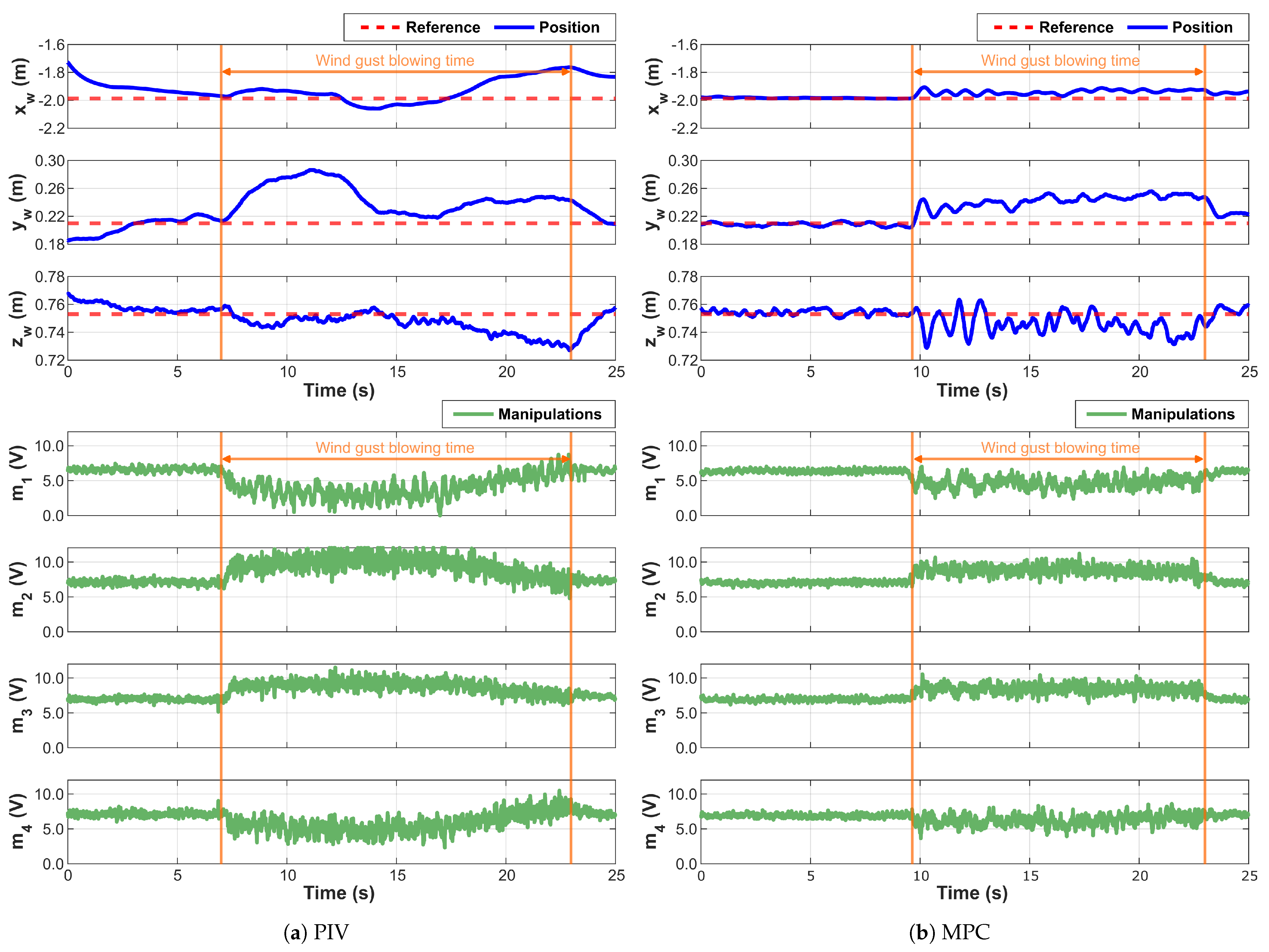
To assess the performance of the MPC and the PIV under external disturbances, the third scenario is considered in the presence of wind gusts. Initially, the quadrotor is in a hovering position according to the inertial frame (Equation (68)).
x w d = 1.987 [ m ] y w d = 0.21 [ m ] z w d = 0.753 [ m ]
A leaf blower with a blowing rate of 900 [m3/h] at a speed of 177 [km/h] is placed at a distance of 3 [m] away at a 45° angle. The duration of the random disturbance applied for the quadrotor under the PIV control structure is 15.96 [s], in which 3193 time steps are collected; this is considering a sample time of 5 [ms]. Meanwhile, the duration of the random disturbance under the MPC control structure is 13.355 [s], which implies the collection of 2672 time steps of 5 [ms]. Table 5 shows the specific time in which the disturbance is applied to the quadrotor under both control structures. As is shown in Figure 7, the wind gusts produced greater disturbance against the PIV method controller than the proposed cascaded MPC. In addition, when using the proposed cascaded MPC, the signal effort presents less fluctuations.
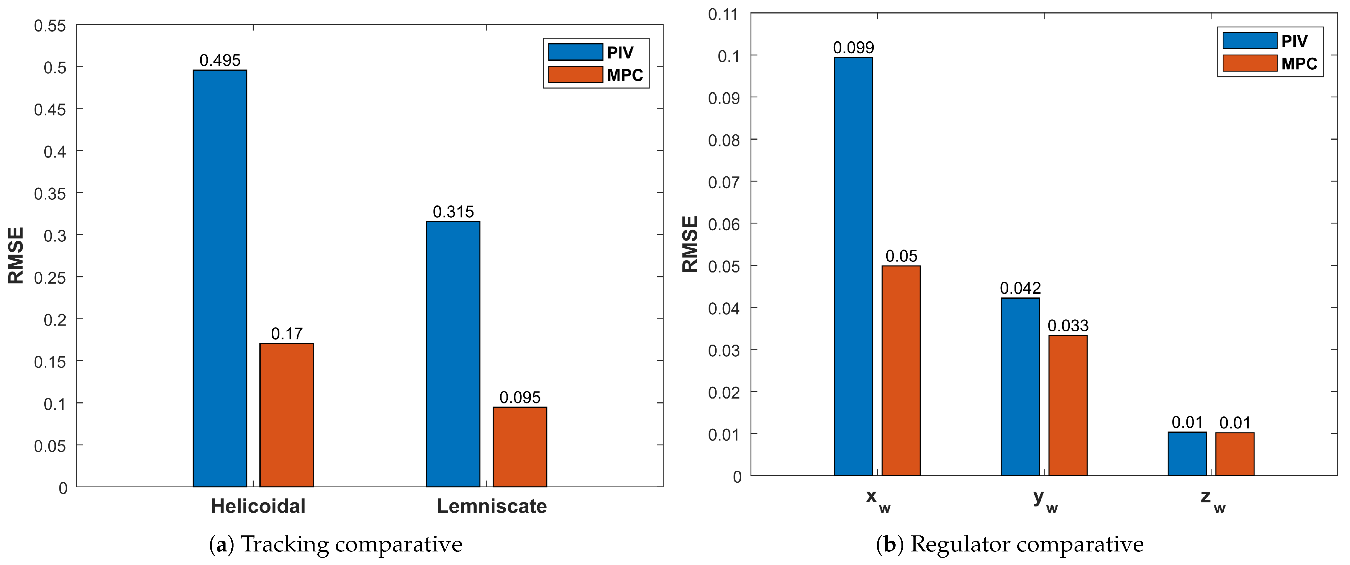
Thus, to verify the efficiency of both controllers, a root-mean-squared error (RMSE) comparison of tracking performance for each scenario is made (Equation (69)).
R M S E = i = 1 n y i d y i 2 n
where n is the number of time steps, y i d is the reference value, and y i is the measured value. Figure 8 shows the RMSE comparison, which includes 10,039 and 9026 collected time steps of 5 [ms] for the helicoidal and lemniscate trajectories, respectively. The lower the RMSE value, the better the tracking performance.
Based on the result of the practical scenarios, it can be concluded that the proposed MPC controller improves the overall tracking performance in comparison with the PIV control method. The RMSE comparison analysis from the experimental results indicates that the proposed cascaded MPC architecture outperforms the PIV method. During the helicoidal trajectory, an RMS value of 0.17 is achieved for the proposed MPC, while 0.495 is obtained using the PIV strategy. Moreover, at the end of the lemniscate trajectory, RMS values of 0.095 and 0.315 are obtained for the proposed MPC and PIV structures, respectively. Therefore, it can be seen that the PIV controller cannot adequately control the quadrotor [52].

6. Conclusions

This paper proposes a multivariable cascaded MPC structure for real-time implementation in quadrotors. The proposed architecture is used to test the translational and attitude control of the QDrone 2 by Quanser®. For tracking control, helicoidal and lemniscate trajectories are chosen to demonstrate the ability of the quadrotor in automatic flight mode. Additionally, for regulatory control, wind gusts are applied to the quadrotor in a hovering position to validate disturbance rejection. For tracking control, using the proposed cascaded MPC architecture, the RMS values are reduced by more than a half. Similarly, lower RMS values for the three positions of the quadrotor are achieved in the presence of external disturbances, especially for x w position, which receives the wind gusts directly. Thus, higher tracking and regulatory performances are obtained. Our future work will be a maneuver control of multiple drones by using the proposed method and applying particle swarm optimization.

Author Contributions

Conceptualization, P.B.-B., D.S. and C.S.; methodology, D.S., M.F., L.E.G.-C., L.J.-M. and C.S.; validation, D.S., L.J.-M. and C.S.; investigation, D.S., M.F., L.E.G.-C. and C.S.; resources, D.S., M.F. and C.S.; writing—original draft, P.B.-B., D.S., L.J.-M. and C.S.; writing—review and editing, D.S., M.F., L.E.G.-C., L.J.-M. and C.S.; supervision, D.S., M.F., L.E.G.-C. and C.S.; project administration, D.S., M.F. and L.E.G.-C. and C.S.; funding acquisition, D.S, M.F. and C.S. All authors have read and agreed to the published version of the manuscript.

Funding

This material is based upon work supported by, or in part by, the U. S. Army Research Laboratory and the U. S. Army Research Office under contract/grant number W911NF2010260.

Data Availability Statement

The data presented in this study are available on request from the corresponding author. The data are not publicly available to provide specific detail upon request.

Acknowledgments

The authors would like to acknowledge the use of the SWARM Lab at the University of the Incarnate Autonomous Vehicle Systems Research Laboratories.

Conflicts of Interest

The authors declare no conflicts of interest.

References

  1. Idrissi, M.; Salami, M.; Annaz, F. A review of quadrotor unmanned aerial vehicles: Applications, architectural design and control algorithms. J. Intell. Robot. Syst. 2022, 104, 22. [Google Scholar] [CrossRef]
  2. Al Tahtawi, A.R.; Yusuf, M. Low-cost quadrotor hardware design with PID control system as flight controller. TELKOMNIKA (Telecommun. Comput. Electron. Control.) 2019, 17, 1923–1930. [Google Scholar] [CrossRef]
  3. Shakeel, T.; Arshad, J.; Jaffery, M.H.; Rehman, A.U.; Eldin, E.T.; Ghamry, N.A.; Shafiq, M. A Comparative Study of Control Methods for X3D Quadrotor Feedback Trajectory Control. Appl. Sci. 2022, 12, 9254. [Google Scholar] [CrossRef]
  4. Rinaldi, M.; Primatesta, S.; Guglieri, G. A comparative study for control of quadrotor uavs. Appl. Sci. 2023, 13, 3464. [Google Scholar] [CrossRef]
  5. Chovancová, A.; Fico, T.; Duchoň, F.; Dekan, M.; Chovanec, L.; Dekanova, M. Control methods comparison for the real quadrotor on an innovative test stand. Appl. Sci. 2020, 10, 2064. [Google Scholar] [CrossRef]
  6. Benaddy, A.; Bouzi, M.; Labbadi, M. Comparison of the different control strategies for Quadrotor Unmanned Aerial Vehicle. In Proceedings of the 2020 International Conference on Intelligent Systems and Computer Vision (ISCV), Fez, Morocco, 9–11 June 2020; pp. 1–6. [Google Scholar]
  7. Kang, C.; Park, B.; Choi, J. Scheduling PID attitude and position control frequencies for time-optimal quadrotor waypoint tracking under unknown external disturbances. Sensors 2021, 22, 150. [Google Scholar] [CrossRef] [PubMed]
  8. Nazin, A.; Alazki, H.; Poznyak, A. Robust Tracking as Constrained Optimization by Uncertain Dynamic Plant: Mirror Descent Method and ASG—Version of Integral Sliding Mode Control. Mathematics 2023, 11, 4112. [Google Scholar] [CrossRef]
  9. Bøhn, E.; Gros, S.; Moe, S.; Johansen, T.A. Reinforcement learning of the prediction horizon in model predictive control. IFAC-PapersOnLine 2021, 54, 314–320. [Google Scholar] [CrossRef]
  10. Veksler, A.; Johansen, T.A.; Borrelli, F.; Realfsen, B. Dynamic positioning with model predictive control. IEEE Trans. Control Syst. Technol. 2016, 24, 1340–1353. [Google Scholar] [CrossRef]
  11. Mohamed, O.; Wang, J.; Al-Duri, B.; Lu, J.; Gao, Q.; Xue, Y.; Liu, X. Predictive control of coal mills for improving supercritical power generation process dynamic responses. In Proceedings of the 2012 IEEE 51st IEEE Conference on Decision and Control (CDC), Maui, HI, USA, 10–13 December 2012; pp. 1709–1714. [Google Scholar]
  12. Polisano, F.; Ryals, A.D.; Pannocchia, G.; Landi, A. MPC based optimization applied to treatment of HCV infections. Comput. Methods Programs Biomed. 2021, 210, 106383. [Google Scholar] [CrossRef]
  13. Bardaro, G.; Bascetta, L.; Ceravolo, E.; Farina, M.; Gabellone, M.; Matteucci, M. MPC-based control architecture of an autonomous wheelchair for indoor environments. Control Eng. Pract. 2018, 78, 160–174. [Google Scholar] [CrossRef]
  14. Skjong, E.; Johansen, T.A.; Molinas, M. Distributed control architecture for real-time model predictive control for system-level harmonic mitigation in power systems. ISA Trans. 2019, 93, 231–243. [Google Scholar] [CrossRef] [PubMed]
  15. Carlet, P.G.; Toso, F.; Favato, A.; Bolognani, S. A speed and current cascade Continuous Control Set Model Predictive Control architecture for synchronous motor drives. In Proceedings of the 2019 IEEE Energy Conversion Congress and Exposition (ECCE), Baltimore, MD, USA, 29 September–3 October 2019; pp. 5682–5688. [Google Scholar]
  16. Palmieri, A.; Rosini, A.; Procopio, R.; Bonfiglio, A. An MPC-sliding mode cascaded control architecture for PV grid-feeding inverters. Energies 2020, 13, 2326. [Google Scholar] [CrossRef]
  17. Kumar, P.; Rawlings, J.B.; Carrette, P. Modeling proportional–integral controllers in tracking and economic model predictive control. J. Process Control 2023, 122, 1–12. [Google Scholar] [CrossRef]
  18. Benotsmane, R.; Vásárhelyi, J. Towards optimization of energy consumption of tello quad-rotor with mpc model implementation. Energies 2022, 15, 9207. [Google Scholar] [CrossRef]
  19. Xue, R.; Dai, L.; Huo, D.; Xie, H.; Sun, Z.; Xia, Y. Compound tracking control based on MPC for quadrotors with disturbances. J. Frankl. Inst. 2022, 359, 7992–8013. [Google Scholar] [CrossRef]
  20. Eskandarpour, A.; Sharf, I. A constrained error-based MPC for path following of quadrotor with stability analysis. Nonlinear Dyn. 2020, 99, 899–918. [Google Scholar] [CrossRef]
  21. Westenberger, J.; De Wagter, C.; de Croon, G.C. Efficient Bang-Bang Model Predictive Control for Quadcopters. Unmanned Syst. 2022, 10, 395–405. [Google Scholar] [CrossRef]
  22. Schlagenhauf, J.; Hofmeier, P.; Bronnenmeyer, T.; Paelinck, R.; Diehl, M. Cascaded nonlinear mpc for realtime quadrotor position tracking. IFAC-PapersOnLine 2020, 53, 7026–7032. [Google Scholar] [CrossRef]
  23. Nan, F.; Sun, S.; Foehn, P.; Scaramuzza, D. Nonlinear MPC for quadrotor fault-tolerant control. IEEE Robot. Autom. Lett. 2022, 7, 5047–5054. [Google Scholar] [CrossRef]
  24. Hanover, D.; Foehn, P.; Sun, S.; Kaufmann, E.; Scaramuzza, D. Performance, precision, and payloads: Adaptive nonlinear mpc for quadrotors. IEEE Robot. Autom. Lett. 2021, 7, 690–697. [Google Scholar] [CrossRef]
  25. Zhao, C.; Wang, D.; Hu, J.; Pan, Q. Nonlinear model predictive control-based guidance algorithm for quadrotor trajectory tracking with obstacle avoidance. J. Syst. Sci. Complex. 2021, 34, 1379–1400. [Google Scholar] [CrossRef]
  26. Pereira, J.C.; Leite, V.J.; Raffo, G.V. Nonlinear model predictive control on SE (3) for quadrotor aggressive maneuvers. J. Intell. Robot. Syst. 2021, 101, 1–15. [Google Scholar] [CrossRef]
  27. Kamel, M.A.; Hafez, A.T.; Yu, X. A review on motion control of unmanned ground and aerial vehicles based on model predictive control techniques. J. Eng. Sci. Mil. Technol. 2018, 2, 10–23. [Google Scholar]
  28. Wang, S.; Polyakov, A.; Zheng, G. Generalized homogenization of linear controllers: Theory and experiment. Int. J. Robust Nonlinear Control 2021, 31, 3455–3479. [Google Scholar] [CrossRef]
  29. Lambert, P.; Reyhanoglu, M. Observer-based sliding mode control of a 2-DOF helicopter system. In Proceedings of the IECON 2018—44th Annual Conference of the IEEE Industrial Electronics Society, Washington, DC, USA, 21–23 October 2018; pp. 2596–2600. [Google Scholar]
  30. Mendez, A.P.; Whidborne, J.F.; Chen, L. Wind Preview-Based Model Predictive Control of Multi-Rotor UAVs Using LiDAR. Sensors 2023, 23, 3711. [Google Scholar] [CrossRef] [PubMed]
  31. Jiang, Y.; Hu, S.; Damaren, C.; Luo, L.; Liu, B. Trajectory Planning with Collision Avoidance for Multiple Quadrotor UAVs Using DMPC. Int. J. Aeronaut. Space Sci. 2023, 24, 1403–1417. [Google Scholar] [CrossRef]
  32. Landolfi, E.; Natale, C. An adaptive cascade predictive control strategy for connected and automated vehicles. Int. J. Adapt. Control Signal Process. 2023, 37, 2725–2751. [Google Scholar] [CrossRef]
  33. Sajjadi, S.; Mehrandezh, M.; Janabi-Sharifi, F. A Cascaded and Adaptive Visual Predictive Control Approach for Real-Time Dynamic Visual Servoing. Drones 2022, 6, 127. [Google Scholar] [CrossRef]
  34. Xu, Z.; Fan, L.; Qiu, W.; Wen, G.; He, Y. A Robust Disturbance-Rejection Controller Using Model Predictive Control for Quadrotor UAV in Tracking Aggressive Trajectory. Drones 2023, 7, 557. [Google Scholar] [CrossRef]
  35. Quanser. Qdrone—Quanser. 2020. Available online: https://www.quanser.com/products/qdrone (accessed on 6 May 2020).
  36. Alaiwi, Y.; Mutlu, A. Modelling, simulation and implementation of autonomous unmanned quadrotor. Mach. Technol. Mater. 2018, 12, 320–325. [Google Scholar]
  37. Kapnopoulos, A.; Alexandridis, A. A cooperative particle swarm optimization approach for tuning an MPC-based quadrotor trajectory tracking scheme. Aerosp. Sci. Technol. 2022, 127, 107725. [Google Scholar] [CrossRef]
  38. Islam, M.; Okasha, M.; Idres, M. Dynamics and control of quadcopter using linear model predictive control approach. In Proceedings of the IOP Conference Series: Materials Science and Engineering; IOP Publishing: Bristol, UK, 2017; Volume 270, p. 012007. [Google Scholar]
  39. Yan, D.; Zhang, W.; Chen, H. Design of a multi-constraint formation controller based on improved MPC and consensus for quadrotors. Aerospace 2022, 9, 94. [Google Scholar] [CrossRef]
  40. Roy, R.; Islam, M.; Sadman, N.; Mahmud, M.A.P.; Gupta, K.D.; Ahsan, M.M. A Review on Comparative Remarks, Performance Evaluation and Improvement Strategies of Quadrotor Controllers. Technologies 2021, 9, 37. [Google Scholar] [CrossRef]
  41. Saeed, A.S.; Younes, A.B.; Islam, S.; Dias, J.; Seneviratne, L.; Cai, G. A review on the platform design, dynamic modeling and control of hybrid UAVs. In Proceedings of the 2015 International Conference on Unmanned Aircraft Systems (ICUAS), Denver, CO, USA, 9–12 June 2015; pp. 806–815. [Google Scholar] [CrossRef]
  42. Zhang, X.; Li, X.; Wang, K.; Lu, Y. A survey of modelling and identification of quadrotor robot. Abstr. Appl. Anal. 2014, 2014, 320526. [Google Scholar] [CrossRef]
  43. Alamir, M. A Pragmatic Story of Model Predictive Control: Self Contained Algorithms and Case-Studies; CreateSpace Independent Publishing Platform: Scotts Valley, CA, USA, 2013. [Google Scholar]
  44. Chen, K.; Zhu, Z.; Zeng, X.; Wang, J. Distributed Observers for State Omniscience with Stochastic Communication Noises. Mathematics 2023, 11, 1997. [Google Scholar] [CrossRef]
  45. Liu, Z.; Yuan, C.; Zhang, Y. Active fault-tolerant control of unmanned quadrotor helicopter using linear parameter varying technique. J. Intell. Robot. Syst. 2017, 88, 415–436. [Google Scholar] [CrossRef]
  46. Mehmet, E. Neural network assisted computationally simple pid control of a quadrotor UAV. IEEE Trans. Ind. Inform. 2011, 7, 354–361. [Google Scholar]
  47. Efe, M.Ö. Battery power loss compensated fractional order sliding mode control of a quadrotor UAV. Asian J. Control 2012, 14, 413–425. [Google Scholar] [CrossRef]
  48. Pi, C.H.; Hu, K.C.; Cheng, S.; Wu, I.C. Low-level autonomous control and tracking of quadrotor using reinforcement learning. Control Eng. Pract. 2020, 95, 104222. [Google Scholar] [CrossRef]
  49. Alkomy, H.; Shan, J. Vibration reduction of a quadrotor with a cable-suspended payload using polynomial trajectories. Nonlinear Dyn. 2021, 104, 3713–3735. [Google Scholar] [CrossRef]
  50. Labbadi, M.; Chatri, C.; Boubaker, S.; Kamel, S. Fixed-Time Controller for Altitude/Yaw Control of Mini-Drones: Real-Time Implementation with Uncertainties. Mathematics 2023, 11, 2703. [Google Scholar] [CrossRef]
  51. Aliyari, M.; Wong, W.K.; Bouteraa, Y.; Najafinia, S.; Fekih, A.; Mobayen, S. Design and implementation of a constrained model predictive control approach for unmanned aerial vehicles. IEEE Access 2022, 10, 91750–91762. [Google Scholar] [CrossRef]
  52. Utkin, A.V.; Utkin, V.A.; Krasnova, S.A. Synthesis of a Control System for a Waste Heat Boiler with Forced Circulation under Restrictions on Control Actions. Mathematics 2022, 10, 2397. [Google Scholar] [CrossRef]
Figure 1. Schematic depiction of the quadrotor coordinate frame configuration.
Mathematics 12 00739 g001
Figure 2. Overall quadrotor control structure.
Mathematics 12 00739 g002
Figure 3. Block diagram of the PIV structure.
Mathematics 12 00739 g003
Figure 4. Block diagram of the cascaded MPC structure.
Mathematics 12 00739 g004
Figure 5. Helicoidal trajectory scenario.
Mathematics 12 00739 g005
Figure 6. Lemniscate trajectory scenario.
Mathematics 12 00739 g006
Figure 7. Disturbance rejection scenario.
Mathematics 12 00739 g007
Figure 8. RMSE comparison.
Mathematics 12 00739 g008
Table 1. Methodology that describes each MPC controller implemented.
MPC Methodology
Input:Actual states of the quadrotor and desired values
Output:Optimal manipulation
1Define the LTI mathematical model of the physical system in state space representation
2Define the sampling time and discretize the state space representation
3Set the sampling instants N for the prediction horizon
4Compute the matrices Φ i , Ψ i and Θ i , i 1 , , N used to represent the N-step-ahead prediction map for LTI systems
5Define weight matrices Q and R
6Determine the saturations
7Compute the online matrices H and F
8Obtain the control law u ˜ o p t and apply to the system the first control input of the best control input sequence
Table 2. Parameters of the drone used for testing.
QDrone 2 Parameters
Dimensions50 × 50 × 15 cm-
Mass1500 g-
Max. Payload300 g-
K v 2100 RPM V -
Max. Continuous Current25 A-
K v , e f f 1295.4   RPM V Effective motor speed constant
W c 2132.6 RPMVoltage-to-angular velocity offset
W f 1004.5 RPMAngular velocity-to-force offset
C t 2.0784 × 10 8   N RPM 2 Motor force constant
F b 0.2046 NMotor force offset
k T 81.0363   N Nm Motor thrust–torque constant
Table 3. PIV tuning parameters.
PIV ParametersPosition PIV x w y w z w Angular PIV ϕ θ ψ Angular Vel. PIV ϕ ˙ θ ˙ ψ ˙
K p π 2 π 2 35 12 12 15 0.188 0.154 0.040
K i 0 0 6 --
K v π 2 π 3 28 0.1 0.1 4 0.003 0.003 0
Table 4. MPC tuning parameters.
MPC ParametersAltitude MPC x w y w Position MPCAttitude MPC
Q matrix10 1000 500 1500 750 1500
R matrix 0.00001 75 50 200 500 250
Prediction horizon N101015
Sample time k 0.25 0.05 0.025
Table 5. Time lapses of the wind disturbance.
QuadrotorStartEnd
Under PIV7.005 s22.965 s
Under MPC9.645 s23 s
Disclaimer/Publisher’s Note: The statements, opinions and data contained in all publications are solely those of the individual author(s) and contributor(s) and not of MDPI and/or the editor(s). MDPI and/or the editor(s) disclaim responsibility for any injury to people or property resulting from any ideas, methods, instructions or products referred to in the content.