Abstract
The selection of the most suitable material is one of the key decisions to be made during the design stage of a manufacturing process. Traditional approaches, such as Ashby maps based on material properties, are widely used in industry. However, in the production of multi-material components, the criteria for the selection can include antagonistic approaches. The aim of this work is to implement a methodology based on the results of process simulations for several materials and to classify them by applying an advanced data analytics method based on machine learning (ML)—in this case, the support vector regression (SVR) or multi-criteria decision-making (MCDM) methodology. Specifically, the multi-criteria optimization and compromise solution (VIKOR) was combined with entropy weighting methods. To achieve this, a finite element model (FEM) was built to evaluate the extrusion force and the die wear during the multi-material co-extrusion process of bimetallic Ti6Al4V-AZ31B billets. After applying SVR and VIKOR in combination with the entropy weighting methodology, a comparison was established based on material selection and the complexity of the methodology used. The results show that the material chosen in both methodologies is very similar, but the MCDM method is easier to implement because there is no need for evaluating the error of the prediction model, and the time required for data preprocessing is less than the time needed when applying SVR. This new methodology is proven to be effective as an alternative to traditional approaches and is aligned with the new trends in industry based on simulation and data analytics.
Keywords:
data analytics; methodologies; multi-material; co-extrusion; FEM; machine learning; SVR; MCDM MSC:
90-11; 90B25; 90B30; 90B50
1. Introduction
In recent years and with the rise of Industry 4.0, simulation and data analytics methodologies have become more relevant due to their capacity for predicting results and being more sustainable compared to traditional approaches. There is an increasing need to develop lighter materials in the aerospace and automotive industries to improve fuel efficiency, reduce environmental impacts, and increase the payloads to be carried out. Multi-material forming has become a solution because of its capacity to reduce weight by joining dissimilar materials and customize the mechanical properties of the final part to fulfill in-service requirements.
Aluminum alloys and carbon-fiber-reinforced composites are widely used in the aerospace industry. However, magnesium alloys have a lower density and a good specific strength [1]; therefore, they could be a good alternative to reduce weight if it were not for their poor corrosion resistance. Because of this, a multi-material component made of magnesium alloys combined with titanium alloys, which has excellent mechanical and physical–chemical properties, together with a very good strength-to-weight ratio and superior corrosion resistance [2], could be the solution to manufacture lighter parts with good mechanical properties and without corrosion problems and thus contribute to reducing the weight of aircraft.
Multi-material forming involves a co-extrusion process to obtain bimetallic billets composed of a cylindrical sleeve and a core made of different materials. Some application cases of multi-material forming processes with two alloys are the studies performed by Fernández et al. [3,4], who analyzed the effects of different co-extrusion process parameters via finite element analysis (FEM) simulations, while using analysis of variance (ANOVA) to determine the most relevant parameters; these authors also investigated the effect of the selection of die material on the co-extrusion process of bimetallic cylindrical billets made of a magnesium alloy core and a titanium alloy sleeve. Other interesting contributions are the studies performed by Negendanka et al. [5], who carried out a study examining diffusion layer formation under different die angle values in a Mg-core and Al-sleeve billet, and by Gall et al. [6], who studied the co-extrusion of bimetallic Al–Mg billets into hollow profiles by means of a finite element method (FEM) simulation together with experiments.
On the other hand, machine learning (ML) [7] has been gaining traction in industry as the preferred method to forecast results and anticipate problems [8] by means of algorithms based on statistical methods to detect patterns from data. The support vector machine (SVM) is one of the most popular supervised learning methods within ML. It was introduced by Vladimir Vapnik [9] in 1995, and its main applications are in classification and regression analysis. For the latter, the implementation of a support vector regression (SVR) module within the SVM to estimate discrete values and thus predict future results is especially interesting. Some examples of SVR applications in industry are the prediction of the laser cutting process cost for AISI316L stainless steel [10], prediction of the cutting force and temperature in bone drilling [11], and prediction of the drilling force for drilling an internal hole in a carbon-fiber-reinforced polymer (CFRP) [12]. When applied to wear prediction, the research performed by Benkedjouh et al. can be highlighted [13].
Apart from ML, there are other approaches that allow decisions to be made in situations where there are several requirements to fulfill in a complex environment involving a large number of variables. Multi-criteria decision-making (MCDM) methods based on multi-objective optimization have been applied to find a compromise solution to this problem. The first MCDM method was applied by Pareto in 1896 [14], with his famous 80/20 principle. Another example is the study by Saaty in 1977 [15], in which multi-criteria models were used to solve problems with conflicting goals. Several MCDM methods have been developed and applied to support decision making in different areas, such as manufacturing process selection [16], supply chain management contract selection [17], and material selection [18]. In this research area, a combination of VIKOR [19] with entropy weighting methods [20,21] has been chosen as an MCDM methodology to establish optimum die material selection. In the study performed by Fernández et al. [22], different ARAS [23], TOPSIS [24], VIKOR, and COPRAS [25] MCDM methods were compared, in conjunction with the AHP [26], standard deviation [27], and entropy weighting methods.
This study developed two methodologies—one based on SVR and the other applying an entropy weighting method together with MCDM VIKOR—for the material selection of the die in a multi-material co-extrusion process to obtain bimetallic billets made of Ti6Al4V-AZ31B. Both methodologies and their results were compared to establish which one gives better results for the proposed problem.
2. Materials and Methods
2.1. Materials, Geometrical Dimensions, and Process Parameters
In this study, a bimetallic billet made of a Ti6Al4V titanium alloy sleeve and an AZ31B magnesium alloy core during the co-extrusion process was analyzed.
Figure 1 shows the co-extrusion setup with the process parameters and initial dimensions.
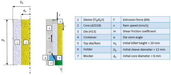
Figure 1.
Co-extrusion setup with process parameters and initial billet dimensions.
The main physical and mechanical properties of Ti6Al4V and AZ31B are shown in Table 1.

Table 1.
Physical and mechanical properties of the titanium alloy Ti6Al4V and the magnesium alloy AZ31B [28,29].
Table 2.
Chemical composition of titanium alloy Ti6Al4V [28].
Table 3.
Chemical composition of magnesium alloy AZ31B [29].
The material candidates for the die were extracted from Daniel et al. [4], whose chemical composition and physical and mechanical properties data are shown in Table 4 and Table 5, respectively.
Table 4.
Chemical composition of die steels [30,31,32,33,34].
Table 5.
Physical and mechanical properties of die steels [35].
The extrusion process parameters evaluated in this research are the following:
- ➢
- Process parameters: ram speed (mm/s) and temperature (°C).
- ➢
- Tooling parameters: die semi-angle (°), shear friction factor, and extrusion ratio (A0/Af).
- ➢
- Geometric parameters: shape factor (H0/D0) and diameter ratio (D0/d0).
In these parameters, A0 and Af are the initial area and the final area of the cross-section of the billet, respectively; D0 and d0 are the initial external diameter and the internal diameter of the sleeve, respectively; and H0 is the initial billet height.
2.2. Finite Element Modeling and Simulation Preparation
The commercial software DEFORM3D© (v11.2) [36] was used to perform the finite element simulations.
All parts were meshed with 7000 tetrahedral elements, and due to the axial symmetry of the process, only one-quarter of the problem was modeled to reduce the computation time and to avoid the generation of heavy database files.
The contact condition among the objects of the simulation was defined as follows: rigid and elastic objects were considered the “masters” (those that deform) and plastic objects were considered “slaves” (those that are deformed). In the case of the interaction between the sleeve and the core, where both objects are plastic, the titanium alloy was defined as the “master” and the magnesium alloy was defined as the “slave”. All materials were assumed to be isotropic throughout the process.
The heat transfer coefficient between the sleeve and the core and between the sleeve and the die was set to 11 N/(s·mm·°C), while that between the extrusion tooling elements and the die was set to 5 N/(s·mm·°C). All objects of the simulation had a 0.02 N/(s·mm·°C) heat transfer coefficient with the air.
The exponential model developed by Wen-juan et al. [37] was used to define the behavior of AZ31B, while the Johnson–Cook constitutive equations [38] were used for the definition of the stress–strain curves of Ti6Al4V.
2.2.1. Tool Wear Model
Archard’s wear model was used to calculate the wear produced on the surface of the die [39,40,41]. This model is based on Equation (1):
where K is the wear coefficient; P is the interface pressure; v is the sliding velocity between the die and the billet; H is the hardness; and a, b, and c are experimentally calibrated coefficients.
The commonly taken value for a and b is 1, while for c, the value is 2 in the case of steel alloys. The equation for calculating the wear coefficient is as follows:
K = 2 × 10⁻⁵.
Taking into account Equation (1), the parameters used to evaluate the wear were the ram speed and friction, as they can influence the sliding velocity, as well as temperature, because it has a direct influence on the stress–strain curves.
2.2.2. FEM Validation
The FEM was validated by using the semi-empirical model proposed by Johnson, which was applied by García et al. [42]. This model is typically used as a reference in extrusion processes to establish an upper limit of the extrusion force. To apply Johnson’s model, it is necessary to obtain the average yield stress of each component in accordance with its volume fraction, as described by Gisbert et al. [43]. The force obtained by the FEM was in good agreement with the semi-empirical model results, with this force being the upper limit of the required forces, as expected. Thus, the FE model can be considered to have been validated.
2.3. Support Vector Regression
The SVM works by finding a hyperplane in a high-dimensional space that best separates data into different classes. It aims to maximize the margin (the distance between the hyperplane and the nearest data points of each class) while minimizing classification errors. The SVM can handle both linear and non-linear classification problems by using various kernel functions. Unlike the SVM used for classification tasks, SVR seeks to find a hyperplane that best fits the data points in a continuous space.
SVR [44] offers the flexibility to define how much error is acceptable in a model and is used to find an appropriate line (or a hyperplane in higher dimensions) to fit the data. Therefore, the goal of SVR is to find a function that approximates the relationship between the input variables and a continuous target variable while minimizing the prediction error.
Another advantage of SVR over linear or logistic regression is the possibility of using different kernel functions, such as polynomial or radial functions, which allows the transformation of data into a higher dimensional space, thereby making it suitable for non-linear problems.
As mentioned before, the idea is to minimize the result of Equation (2), while taking into account the constraints of Equations (3)–(5), as it is shown in Figure 2:
where ε is the margin of error; ξ is the deviation from ε, which is also called the tolerance margin; and w is the classification vector. C is known as the regularized parameter.
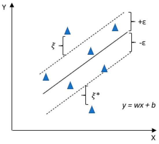
Figure 2.
Two-dimensional hyperplane representation.
The prediction error can be calculated in different ways. One of the most representative is by using the determination factor (R2), which shows the quality of the correlation between the real measured data and the value predicted by Equation (6). A more precise correlation will be obtained when the value of the determination factor is nearer to 100%. The calculation is as follows:
where is the measurement data, is the predicted magnitude in accordance with SVR, is the mean of the measurement data, and is the mean of the prediction.
2.4. Entropy Method
The entropy method [21,22] is classified within the category of objective weighting methods, and it is applicable when the data of a decision matrix are known. Entropy is a measure of randomness and disorder in the universe.
Starting with the decision matrix D, the projected outcomes pij are calculated by means of Equation (7):
where n is the number of criteria and m is the number of alternatives.
The entropy measure of the projected outcomes is obtained as shown in Equation (8):
with k = 1/ln(m).
The objective weight-based definition is calculated according to Equation (9):
2.5. VIKOR Method
VIKOR [45,46] stands for VIseKriterijumska Optimizacija I Kompromisno Resenje, which means multi-criteria optimization and compromise solution.
This methodology is based on the concept that the compromise solution is the one that is at the minimum distance from the ideal solution while, at the same time, at the maximum distance from the anti-ideal solution.
One big difference from the SVM is that VIKOR does not require the calculation of the error because there is no prediction and therefore there is nothing to compare. Instead, VIKOR requires a validation step before declaring the compromise solution that is feasible by fulfilling the “acceptable advantage” and “acceptable stability in decision making” conditions.
Other advantages of using the VIKOR method are the following:
- ➢
- The ability to inmmediately recognize the proper alternative;
- ➢
- A decrease in the number of pairwise comparisons required.
After the criteria to be evaluated are defined, a decision matrix (D) is built:
At this point, the values of the best and the worst for each criterion rating of the decision matrix are obtained as follows:
when the objective is to maximize the criteria.
when the objective is to minimize the criteria.
Where b = 1 …m, with m being the number of criteria that is taken into account, and i = 1 …n, with n being the number of alternatives.
The Utility measure (Sj) and the Regret measure (Rj) are calculated according to Equations (10) and (11):
where Wb are the weight values obtained in this study after applying the entropy weighting methods explained above.
The index Q can be obtained by using Equation (12):
where
In this equation, υ is a parameter that represents the type of voting used during the process (υ > 0.5 means “vote by majority rule”, υ = 0.5 means “vote by consensus”, and υ < 0.5 means “with vote”).
The lowest Qa value indicates the best alternative solution, and it can be recommended if the following conditions are satisfied:
The “acceptable advantage” condition means that Q(a″) − Q(a′) DQ, with a″ being the alternative in the second position in the ranking list by Qa and a′ being the first one. DQ is defined according to Equation (13):
where n is the number or alternatives.
Finally, the “acceptable stability in decision making” condition implies that the a’ alternative must also be the best ranked for Sj and/or Rj. If one of the conditions is not fulfilled, then a set of compromise solutions is proposed.
2.6. Methodology
Two different methodologies were proposed for the selection of the optimum die material in order to obtain the minimum extrusion force and die wear. The methodology steps are shown in the flowchart in Figure 3.
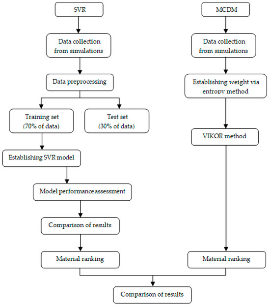
Figure 3.
Methodology flowchart.
The criteria for the final result comparison are as follows:
- ➢
- Simplicity;
- ➢
- Amount of data obtained from the simulations;
- ➢
- Time consumption.
The prediction was carried out using the Python software [47].
3. Results
In this study, a set of simulations for a multi-material co-extrusion process were performed by using the commercial software DEFORM3D© (v11.2), followed by the application of two different methodologies, to choose the best die material to obtain the minimum extrusion force and the minimum wear during the process. For the list of simulations carried out in the present work, see Table A1 in Appendix A.
3.1. SVR Methodology
As explained above, a dataset was obtained for the parameters listed in Table 6, and for each material and each parameter to be predicted, several dataframes were obtained by using the “pandas” together with the “sklearn” libraries.
Table 6.
Ranking of process parameters’ influence on extrusion force.
Using the “RFE” module for Regression Feature Selection from “sklearn.feature_selection”, together with the “SVR” module from “sklearn.svm”, the process parameters were ranked according to their influence on the extrusion force, as shown in Table 6.
Taking into account these results, it can be concluded that friction is the most important process parameter, while temperature is the least important one. This conclusion is in good agreement with the findings reported by Fernández et al. [3,4], who performed a deeper analysis of the influence of each process parameter on the extrusion force.
As there is no clear pattern regarding the influence of the process parameters and their influence is clearly dependent on the die material, all the parameters were implemented in the prediction model.
For the prediction model of the extrusion force, the dataframes for each material were split into two groups—one for training and one for testing—using the “train_test_split” function from the “sklearn.model_selection” module, with the test size being 0.3.
After applying the “LinearRegression” function from “sklearn.linear_model” to build the prediction model using the training data, the model was evaluated using the test data. The determination factor (R2) for each material is shown in Table 7.
Table 7.
Determination factor (R2) for the extrusion force in the linear regression model.
Figure 4, Figure 5, Figure 6, Figure 7 and Figure 8 show the comparisons between the simulation values and the prediction values.
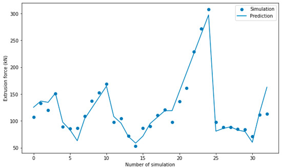
Figure 4.
Comparison of AISI316 extrusion force prediction and simulation values.
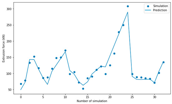
Figure 5.
Comparison of H13 extrusion force prediction and simulation values.
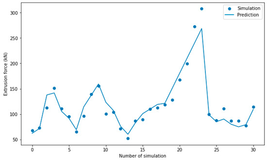
Figure 6.
Comparison of 25CrMo4 extrusion force prediction and simulation values.
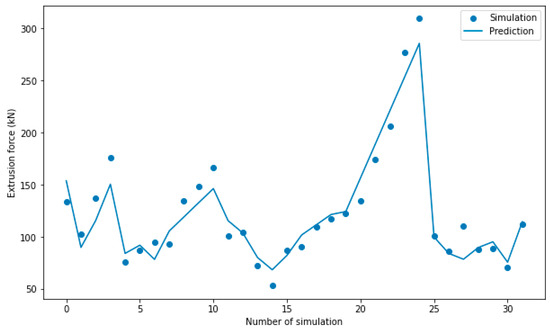
Figure 7.
Comparison of AISI52100 extrusion force prediction and simulation values.
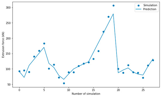
Figure 8.
Comparison of AISI3310 extrusion force prediction and simulation values.
By using the prediction model for each die material, a larger number of results for the extrusion force could be compared without the need to perform more simulations. Table 8 shows the ranking of the die materials as a function of the times that their prediction value for the extrusion force was the lowest.
Table 8.
Ranking of die materials as a function of the times that the lowest extrusion force was produced.
If the minimum extrusion force was the only requirement for the selection of die materials, AISI3310 would be the chosen material, followed by AISI316 and H13, which shared the second position in the ranking.
The SVR methodology was then applied for wear prediction with the following modification:
Due to the variation in the results, it was not possible to apply a linear regression model and so a polynomial one had to be used. To produce a polynomial regression model, it was necessary to import the “PolynomialFeatures” module from the “sklearn.preprocessing” library to generate a new feature matrix consisting of all the polynomial combinations of the features with a degree less than or equal to the specified degree (in this case, a two-degree polynomial function was used).
Table 9 and Table 10 show the ranking of the process parameters and the determination factor (R2) for the wear model.
Table 9.
Ranking of process parameters for die wear.
Table 10.
Determination factor (R2) for the extrusion force in the polynomial regression model.
The conclusion is in good agreement with the findings reported by Fernández et al. [4], who performed a deeper analysis of the influence of each process parameter on the die wear.
The prediction model for the die wear was not as accurate as the one for the extrusion force. This could be due to the fact that the number of simulations performed to obtain the wear distribution was lower than for that for the extrusion force because Archard’s wear model only takes into account temperature, friction, and ram speed, as mentioned in Section 2.2.1.
Figure 9, Figure 10, Figure 11, Figure 12 and Figure 13 show the comparisons between the simulation values and the prediction values.
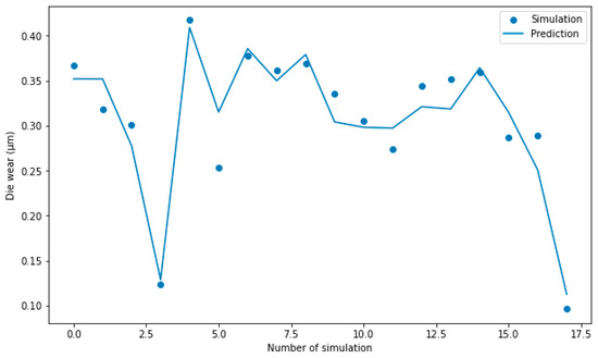
Figure 9.
Comparison of AISI316 die wear prediction and simulation values.
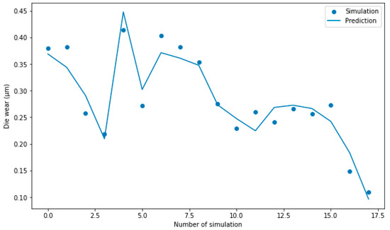
Figure 10.
Comparison of H13 die wear prediction and simulation values.
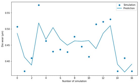
Figure 11.
Comparison of 25CrMo4 die wear prediction and simulation values.
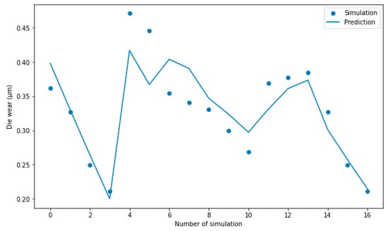
Figure 12.
Comparison of AISI52100 die wear prediction and simulation values.
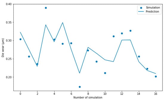
Figure 13.
Comparison of AISI3310 die wear prediction and simulation values.
Table 11 shows the ranking of the die materials as a function of the times that their prediction value for the die wear was the lowest value.
Table 11.
Ranking of die materials as a function of the times that the minimum wear in the die was produced.
Finally, a crosscheck between Table 8 and Table 11 was performed to rank the die materials and find the one that best fulfills the requirements of minimum extrusion force and minimum die wear, and the results are shown in Table 12.
Table 12.
Ranking of die materials as a function of fulfilling the requirements of minimum extrusion force and minimum die wear.
In both rankings, AISI3310 is the best choice to reduce the extrusion force and die wear. AISI316 and H13 have the same ranking position with regard to the extrusion force but not with regard to the die wear, and the reason is because, in the final ranking, AISI316 is ranked better than H13. The die materials that can be rejected as feasible options are AISI52100 and 25CrMo4.
3.2. MCDM Methodology
As explained in Section 3, a dataset was obtained from the simulations listed in Table A1. In the MCDM methodology, weights were calculated by means of the entropy method and, afterwards, the VIKOR method was applied to classify the different materials based on the criteria rating values.
For the entropy method, the decision matrix D was obtained based on the results for each simulation listed in Table A1 regarding the extrusion force and die wear.
| 86.019 | 136.529 | 228.511 | 307.324 | 97.898 | 88.621 | 88.040 | 84.512 | 83.759 | 0.367 | 0.318 | 0.302 | 0.124 | 0.417 | 0.253 | 0.378 | 0.361 | 0.370 |
| 86.153 | 124.955 | 227.644 | 307.783 | 98.095 | 88.706 | 88.140 | 84.799 | 83.850 | 0.379 | 0.382 | 0.257 | 0.219 | 0.414 | 0.271 | 0.404 | 0.381 | 0.354 |
| 95.608 | 128.196 | 199.579 | 307.520 | 100.048 | 87.505 | 111.049 | 87.149 | 86.484 | 0.361 | 0.327 | 0.250 | 0.211 | 0.471 | 0.445 | 0.354 | 0.341 | 0.345 |
| 87.120 | 134.333 | 206.128 | 309.397 | 100.654 | 86.238 | 110.203 | 88.307 | 88.602 | 0.507 | 0.369 | 0.410 | 0.452 | 0.573 | 0.462 | 0.430 | 0.436 | 0.428 |
| 92.531 | 132.578 | 221.350 | 306.154 | 100.708 | 87.422 | 112.221 | 89.296 | 87.588 | 0.304 | 0.257 | 0.281 | 0.236 | 0.389 | 0.303 | 0.291 | 0.292 | 0.173 |
From D, the normalized matrix was obtained by means of Equation (7):
| 0.1923 | 0.2079 | 0.2110 | 0.1998 | 0.1968 | 0.2021 | 0.1727 | 0.1947 | 0.1947 | 0.1913 | 0.1925 | 0.2011 | 0.1000 | 0.1842 | 0.1459 | 0.2035 | 0.1993 | 0.2214 |
| 0.1926 | 0.1903 | 0.2102 | 0.2001 | 0.1972 | 0.2023 | 0.1729 | 0.1954 | 0.1949 | 0.1977 | 0.2311 | 0.1717 | 0.1764 | 0.1829 | 0.1563 | 0.2175 | 0.2105 | 0.2118 |
| 0.2137 | 0.1952 | 0.1842 | 0.1999 | 0.2011 | 0.1996 | 0.2179 | 0.2008 | 0.2010 | 0.1884 | 0.1978 | 0.1667 | 0.1701 | 0.2078 | 0.2568 | 0.1908 | 0.1881 | 0.2067 |
| 0.1947 | 0.2046 | 0.1903 | 0.2011 | 0.2024 | 0.1967 | 0.2162 | 0.2034 | 0.2059 | 0.2642 | 0.2233 | 0.2733 | 0.3639 | 0.2532 | 0.2665 | 0.2315 | 0.2407 | 0.2565 |
| 0.2068 | 0.2019 | 0.2043 | 0.1990 | 0.2025 | 0.1994 | 0.2202 | 0.2057 | 0.2036 | 0.1584 | 0.1553 | 0.1871 | 0.1897 | 0.1719 | 0.1744 | 0.1567 | 0.1614 | 0.1037 |
Then, the entropy array (Ej) was calculated by applying Equation (8):
Ej = [0.999418867 0.999681506 0.999085371 0.999996437 0.999952024 0.999966715 0.996102816 0.999852667 0.999839187 0.990960752 0.99430503 0.989129167 0.944884512 0.993690857 0.979914551 0.994771731 0.99470602 0.976990905]
The weights are presented in Table 13.
Table 13.
Entropy method weights.
Using the VIKOR method, the best and worst values for each criterion were obtained directly from the decision matrix D.
| 86.019 | 136.529 | 228.511 | 307.324 | 97.898 | 88.621 | 88.040 | 84.512 | 83.759 | 0.367 | 0.318 | 0.302 | 0.124 | 0.417 | 0.253 | 0.378 | 0.361 | 0.370 | |
| 86.153 | 124.955 | 227.644 | 307.783 | 98.095 | 88.706 | 88.140 | 84.799 | 83.850 | 0.379 | 0.382 | 0.257 | 0.219 | 0.414 | 0.271 | 0.404 | 0.381 | 0.354 | |
| 95.608 | 128.196 | 199.579 | 307.520 | 100.048 | 87.505 | 111.049 | 87.149 | 86.484 | 0.361 | 0.327 | 0.250 | 0.211 | 0.471 | 0.445 | 0.354 | 0.341 | 0.345 | |
| 87.120 | 134.333 | 206.128 | 309.397 | 100.654 | 86.238 | 110.203 | 88.307 | 88.602 | 0.507 | 0.369 | 0.410 | 0.452 | 0.573 | 0.462 | 0.430 | 0.436 | 0.428 | |
| 92.531 | 132.578 | 221.350 | 306.154 | 100.708 | 87.422 | 112.221 | 89.296 | 87.588 | 0.304 | 0.257 | 0.281 | 0.236 | 0.389 | 0.303 | 0.291 | 0.292 | 0.173 | |
| 447.431 | 656.591 | 1083.212 | 1538.178 | 497.402 | 438.492 | 509.653 | 434.063 | 430.283 | 1.918 | 1.652 | 1.499 | 1.242 | 2.265 | 1.735 | 1.856 | 1.812 | 1.669 | |
| fi* | 86.019 | 124.955 | 199.579 | 306.154 | 97.898 | 86.238 | 88.040 | 84.512 | 83.759 | 0.304 | 0.257 | 0.250 | 0.124 | 0.389 | 0.253 | 0.291 | 0.292 | 0.173 |
| fi- | 95.608 | 136.529 | 228.511 | 309.397 | 100.708 | 88.706 | 112.221 | 89.296 | 88.602 | 0.507 | 0.382 | 0.410 | 0.452 | 0.573 | 0.462 | 0.430 | 0.436 | 0.428 |
The Utility measure (Sj) and the Regret measure (Rj) were then obtained:
| Sj | Ri | ||
|---|---|---|---|
| 0.23758265 | 0.12075866 | ||
| 0.36022622 | 0.11092085 | ||
| 0.44932592 | 0.1258087 | ||
| 0.98459134 | 0.37557176 | ||
| 0.21183731 | 0.12764252 | ||
| S* | 0.21183731 | R* | 0.11092085 |
| S− | 0.98459134 | R− | 0.37557176 |
Using the values S*, S−, R*, and R−, together with the assumption of vote by consensus (υ = 0.5), the index Q was calculated:
| Qi | |
|---|---|
| AISI3310 | 0.03524455 |
| H13 | 0.09601303 |
| AISI52100 | 0.18179111 |
| 25CrMo4 | 1 |
| AISI3310 | 0.03159193 |
Using the VIKOR method, the index Q was ranked from the lowest to the highest value. The best material to obtain the minimum extrusion force and the minimum die wear is AISI3310. But before recommending this material as the best compromise solution, the conditions of “acceptable advantages” and “acceptable stability in decision making” have to be fulfilled.
In this case, DQ = 0.25 according to Equation (13).
| Q(2) − Q(1) = 0.0365261 |
| Q(3) − Q(1) = 0.0644211 |
| Q(4) − Q(1) = 0.15019917 |
| Q(5) − Q(1) = 0.96840807 > DQ |
| Q(1) = S* |
As only the second condition was fulfilled, a set of compromise solutions was ranked, and the results are presented in Table 14.
Table 14.
VIKOR ranking of die materials.
4. Discussion
In this paper, two methodologies are proposed to choose the best material for the die in a multi-material coextrusion process, taking into account that the process has to fulfill the requirements of minimum extrusion force and minimum die wear.
The first methodology proposed is an SVR methodology based on the SVM. The main advantage of this methodology is that the prediction model obtained during the process allows engineers to predict the outcomes when varying the process parameters. On the other hand, the disadvantages are the number of simulations needed to obtain a good prediction model and, depending on the results of those simulations, the complexity of obtaining the prediction model, which can be very high.
The second methodology is the MCDM methodology, which allows the selection of the best die material with a smaller number of simulations than the SVR methodology and without having to consider the accuracy or complexity of prediction models. Also, it is less time-consuming because the entropy and VIKOR methods can be applied directly to the data, and there is no need to have knowledge in programming languages like Python.
The results for the top three materials selected are the same regardless of the methodology applied. Therefore, if there is no need to apply other values to the parameters to obtain a prediction model to forecast the results, the recommended methodology for die material selection is the MCDM methodology due to its simplicity and the time saved in implementing it because there is no need for data preprocessing, nor there is a need for programming or statistical knowledge to interpret the results of the obtained model. In addition, MCDM is more scalable due to the fact that the SVM needs to re-evaluate the prediction model with new data to ensure the accuracy of the results while making certain that the prediction error is not increased.
Finally, for future research, it would be interesting to conduct a comparison among different machine learning methods to obtain a more robust prediction model not only for the wear but also for other parameters, such as the damage factor, mean stresses, and resultant microstructure.
Author Contributions
Conceptualization, D.F., Á.R.-P. and A.M.C.; methodology, D.F.; formal analysis, D.F., Á.R.-P. and A.M.C.; investigation, D.F., Á.R.-P. and A.M.C.; resources, Á.R.-P. and A.M.C.; writing—original draft preparation, D.F.; writing—review and editing, Á.R.-P. and A.M.C.; supervision, Á.R.-P. and A.M.C.; project administration, Á.R.-P. and A.M.C.; funding acquisition, Á.R.-P. and A.M.C. All authors have read and agreed to the published version of the manuscript.
Funding
This research was funded within the framework of the “Doctorate Program in Industrial Technologies” of the UNED and by the project 2021V/-TAJOV/006 (awarded as part of the call for UNED Research Projects for “Young Talents 2021”).
Data Availability Statement
The raw/processed data required to reproduce these findings cannot be shared at this time as the data also form part of an ongoing study.
Acknowledgments
We would like to extend our gratitude to the Research Group of the UNED “Industrial Production and Manufacturing Engineering (IPME)” and the Industrial Research Group “Advanced Failure Prognosis for Engineering Applications”.
Conflicts of Interest
The authors declare no conflicts of interest. The funders had no role in the design of the study; in the collection, analyses, or interpretation of data; in the writing of the manuscript; or in the decision to publish the results.
Appendix A
Table A1.
List of simulations performed by using DEFORM3D© (v11.2).
Table A1.
List of simulations performed by using DEFORM3D© (v11.2).
| Simulation | Material | Ram Speed (mm/s) | Core Diameter (mm) | Billet Height (H) | Temperature (° C) | Friction | Die Semi-Angle (°) | Extrusion Ratio |
|---|---|---|---|---|---|---|---|---|
| 1 | AISI316 | 2 | 5 | 20 | 200 | 0.2 | 30 | 1.78 |
| 2 | AISI316 | 2 | 6 | 15 | 100 | 0.2 | 30 | 2.25 |
| 3 | AISI316 | 2 | 7 | 25 | 100 | 0.3 | 30 | 1.44 |
| 4 | AISI316 | 3 | 6 | 15 | 200 | 0.3 | 15 | 2.25 |
| 5 | AISI316 | 3 | 7 | 15 | 300 | 0.2 | 45 | 1.44 |
| 6 | AISI316 | 2 | 6 | 20 | 200 | 0.1 | 30 | 1.78 |
| 7 | AISI316 | 2 | 6 | 20 | 200 | 0.1 | 15 | 1.78 |
| 8 | AISI316 | 2 | 6 | 20 | 200 | 0.1 | 45 | 1.78 |
| 9 | AISI316 | 2 | 6 | 20 | 200 | 0.1 | 60 | 1.78 |
| 10 | AISI316 | 2 | 6 | 20 | 200 | 0.1 | 75 | 1.78 |
| 11 | AISI316 | 2 | 6 | 20 | 200 | 0.1 | 90 | 1.78 |
| 12 | AISI316 | 2 | 2 | 20 | 200 | 0.1 | 30 | 1.78 |
| 13 | AISI316 | 2 | 4 | 20 | 200 | 0.1 | 30 | 1.78 |
| 14 | AISI316 | 2 | 8 | 20 | 200 | 0.1 | 30 | 1.78 |
| 15 | AISI316 | 2 | 10 | 20 | 200 | 0.1 | 30 | 1.78 |
| 16 | AISI316 | 2 | 6 | 15 | 200 | 0.1 | 30 | 1.78 |
| 17 | AISI316 | 2 | 6 | 25 | 200 | 0.1 | 30 | 1.78 |
| 18 | AISI316 | 2 | 6 | 30 | 200 | 0.1 | 30 | 1.78 |
| 19 | AISI316 | 2 | 6 | 35 | 200 | 0.1 | 30 | 1.78 |
| 20 | AISI316 | 2 | 6 | 20 | 200 | 0.2 | 30 | 1.78 |
| 21 | AISI316 | 2 | 6 | 20 | 200 | 0.3 | 30 | 1.78 |
| 22 | AISI316 | 2 | 6 | 20 | 200 | 0.4 | 30 | 1.78 |
| 23 | AISI316 | 2 | 6 | 20 | 200 | 0.5 | 30 | 1.78 |
| 24 | AISI316 | 2 | 6 | 20 | 200 | 0.6 | 30 | 1.78 |
| 25 | AISI316 | 2 | 6 | 20 | 200 | 0.7 | 30 | 1.78 |
| 26 | AISI316 | 2 | 6 | 20 | 100 | 0.1 | 30 | 1.78 |
| 27 | AISI316 | 2 | 6 | 20 | 300 | 0.1 | 30 | 1.78 |
| 28 | AISI316 | 1 | 6 | 20 | 300 | 0.1 | 30 | 1.78 |
| 29 | AISI316 | 3 | 6 | 20 | 300 | 0.1 | 30 | 1.78 |
| 30 | AISI316 | 4 | 6 | 20 | 300 | 0.1 | 30 | 1.78 |
| 31 | AISI316 | 2 | 6 | 20 | 200 | 0.1 | 30 | 1.44 |
| 32 | AISI316 | 2 | 6 | 20 | 200 | 0.1 | 30 | 2.25 |
| 33 | AISI316 | 2 | 6 | 20 | 200 | 0.1 | 30 | 2.94 |
| 34 | H13 | 2 | 5 | 15 | 100 | 0.1 | 15 | 1.44 |
| 35 | H13 | 2 | 6 | 25 | 300 | 0.1 | 15 | 1.78 |
| 36 | H13 | 3 | 5 | 15 | 300 | 0.3 | 30 | 1.78 |
| 37 | H13 | 3 | 6 | 25 | 100 | 0.2 | 45 | 1.44 |
| 38 | H13 | 3 | 7 | 25 | 200 | 0.1 | 30 | 2.25 |
| 39 | H13 | 2 | 6 | 20 | 200 | 0.1 | 30 | 1.78 |
| 40 | H13 | 2 | 6 | 20 | 200 | 0.1 | 15 | 1.78 |
| 41 | H13 | 2 | 6 | 20 | 200 | 0.1 | 45 | 1.78 |
| 42 | H13 | 2 | 6 | 20 | 200 | 0.1 | 60 | 1.78 |
| 43 | H13 | 2 | 6 | 20 | 200 | 0.1 | 75 | 1.78 |
| 44 | H13 | 2 | 6 | 20 | 200 | 0.1 | 90 | 1.78 |
| 45 | H13 | 2 | 2 | 20 | 200 | 0.1 | 30 | 1.78 |
| 46 | H13 | 2 | 4 | 20 | 200 | 0.1 | 30 | 1.78 |
| 47 | H13 | 2 | 8 | 20 | 200 | 0.1 | 30 | 1.78 |
| 48 | H13 | 2 | 10 | 20 | 200 | 0.1 | 30 | 1.78 |
| 49 | H13 | 2 | 6 | 15 | 200 | 0.1 | 30 | 1.78 |
| 50 | H13 | 2 | 6 | 25 | 200 | 0.1 | 30 | 1.78 |
| 51 | H13 | 2 | 6 | 30 | 200 | 0.1 | 30 | 1.78 |
| 52 | H13 | 2 | 6 | 35 | 200 | 0.1 | 30 | 1.78 |
| 53 | H13 | 2 | 6 | 20 | 200 | 0.2 | 30 | 1.78 |
| 54 | H13 | 2 | 6 | 20 | 200 | 0.3 | 30 | 1.78 |
| 55 | H13 | 2 | 6 | 20 | 200 | 0.4 | 30 | 1.78 |
| 56 | H13 | 2 | 6 | 20 | 200 | 0.5 | 30 | 1.78 |
| 57 | H13 | 2 | 6 | 20 | 200 | 0.6 | 30 | 1.78 |
| 58 | H13 | 2 | 6 | 20 | 200 | 0.7 | 30 | 1.78 |
| 59 | H13 | 2 | 6 | 20 | 100 | 0.1 | 30 | 1.78 |
| 60 | H13 | 2 | 6 | 20 | 300 | 0.1 | 30 | 1.78 |
| 61 | H13 | 1 | 6 | 20 | 300 | 0.1 | 30 | 1.78 |
| 62 | H13 | 3 | 6 | 20 | 300 | 0.1 | 30 | 1.78 |
| 63 | H13 | 4 | 6 | 20 | 300 | 0.1 | 30 | 1.78 |
| 64 | H13 | 2 | 6 | 20 | 200 | 0.1 | 30 | 1.44 |
| 65 | H13 | 2 | 6 | 20 | 200 | 0.1 | 30 | 2.25 |
| 66 | H13 | 2 | 6 | 20 | 200 | 0.1 | 30 | 2.94 |
| 67 | AISI52100 | 2 | 5 | 15 | 100 | 0.1 | 15 | 1.44 |
| 68 | AISI52100 | 2 | 6 | 25 | 300 | 0.1 | 15 | 1.78 |
| 69 | AISI52100 | 3 | 5 | 15 | 300 | 0.3 | 30 | 1.78 |
| 70 | AISI52100 | 3 | 6 | 25 | 100 | 0.2 | 45 | 1.44 |
| 71 | AISI52100 | 3 | 7 | 25 | 200 | 0.1 | 30 | 2.25 |
| 72 | AISI52100 | 2 | 6 | 20 | 200 | 0.1 | 30 | 1.78 |
| 73 | AISI52100 | 2 | 6 | 20 | 200 | 0.1 | 15 | 1.78 |
| 74 | AISI52100 | 2 | 6 | 20 | 200 | 0.1 | 45 | 1.78 |
| 75 | AISI52100 | 2 | 6 | 20 | 200 | 0.1 | 60 | 1.78 |
| 76 | AISI52100 | 2 | 6 | 20 | 200 | 0.1 | 75 | 1.78 |
| 77 | AISI52100 | 2 | 2 | 20 | 200 | 0.1 | 30 | 1.78 |
| 78 | AISI52100 | 2 | 4 | 20 | 200 | 0.1 | 30 | 1.78 |
| 79 | AISI52100 | 2 | 8 | 20 | 200 | 0.1 | 30 | 1.78 |
| 80 | AISI52100 | 2 | 10 | 20 | 200 | 0.1 | 30 | 1.78 |
| 81 | AISI52100 | 2 | 6 | 15 | 200 | 0.1 | 30 | 1.78 |
| 82 | AISI52100 | 2 | 6 | 25 | 200 | 0.1 | 30 | 1.78 |
| 83 | AISI52100 | 2 | 6 | 30 | 200 | 0.1 | 30 | 1.78 |
| 84 | AISI52100 | 2 | 6 | 35 | 200 | 0.1 | 30 | 1.78 |
| 85 | AISI52100 | 2 | 6 | 20 | 200 | 0.2 | 30 | 1.78 |
| 86 | AISI52100 | 2 | 6 | 20 | 200 | 0.3 | 30 | 1.78 |
| 87 | AISI52100 | 2 | 6 | 20 | 200 | 0.4 | 30 | 1.78 |
| 88 | AISI52100 | 2 | 6 | 20 | 200 | 0.5 | 30 | 1.78 |
| 89 | AISI52100 | 2 | 6 | 20 | 200 | 0.6 | 30 | 1.78 |
| 90 | AISI52100 | 2 | 6 | 20 | 200 | 0.7 | 30 | 1.78 |
| 91 | AISI52100 | 2 | 6 | 20 | 100 | 0.1 | 30 | 1.78 |
| 92 | AISI52100 | 2 | 6 | 20 | 300 | 0.1 | 30 | 1.78 |
| 93 | AISI52100 | 1 | 6 | 20 | 300 | 0.1 | 30 | 1.78 |
| 94 | AISI52100 | 3 | 6 | 20 | 300 | 0.1 | 30 | 1.78 |
| 95 | AISI52100 | 4 | 6 | 20 | 300 | 0.1 | 30 | 1.78 |
| 96 | AISI52100 | 2 | 6 | 20 | 200 | 0.1 | 30 | 1.44 |
| 97 | AISI52100 | 2 | 6 | 20 | 200 | 0.1 | 30 | 2.25 |
| 98 | 25CrMo4 | 2 | 6 | 20 | 200 | 0.3 | 45 | 1.44 |
| 99 | 25CrMo4 | 2 | 7 | 15 | 200 | 0.1 | 45 | 1.78 |
| 100 | 25CrMo4 | 3 | 5 | 25 | 200 | 0.2 | 15 | 1.44 |
| 101 | 25CrMo4 | 3 | 7 | 20 | 100 | 0.3 | 15 | 1.78 |
| 102 | 25CrMo4 | 2 | 6 | 20 | 300 | 0.1 | 30 | 1.78 |
| 103 | 25CrMo4 | 2 | 6 | 20 | 200 | 0.1 | 30 | 1.78 |
| 104 | 25CrMo4 | 2 | 6 | 20 | 200 | 0.1 | 15 | 1.78 |
| 105 | 25CrMo4 | 2 | 6 | 20 | 200 | 0.1 | 45 | 1.78 |
| 106 | 25CrMo4 | 2 | 6 | 20 | 200 | 0.1 | 60 | 1.78 |
| 107 | 25CrMo4 | 2 | 6 | 20 | 200 | 0.1 | 75 | 1.78 |
| 108 | 25CrMo4 | 2 | 6 | 20 | 200 | 0.1 | 90 | 1.78 |
| 109 | 25CrMo4 | 2 | 2 | 20 | 200 | 0.1 | 30 | 1.78 |
| 110 | 25CrMo4 | 2 | 4 | 20 | 200 | 0.1 | 30 | 1.78 |
| 111 | 25CrMo4 | 2 | 8 | 20 | 200 | 0.1 | 30 | 1.78 |
| 112 | 25CrMo4 | 2 | 10 | 20 | 200 | 0.1 | 30 | 1.78 |
| 113 | 25CrMo4 | 2 | 6 | 15 | 200 | 0.1 | 30 | 1.78 |
| 114 | 25CrMo4 | 2 | 6 | 25 | 200 | 0.1 | 30 | 1.78 |
| 115 | 25CrMo4 | 2 | 6 | 30 | 200 | 0.1 | 30 | 1.78 |
| 116 | 25CrMo4 | 2 | 6 | 35 | 200 | 0.1 | 30 | 1.78 |
| 117 | 25CrMo4 | 2 | 6 | 20 | 200 | 0.2 | 30 | 1.78 |
| 118 | 25CrMo4 | 2 | 6 | 20 | 200 | 0.3 | 30 | 1.78 |
| 119 | 25CrMo4 | 2 | 6 | 20 | 200 | 0.4 | 30 | 1.78 |
| 120 | 25CrMo4 | 2 | 6 | 20 | 200 | 0.5 | 30 | 1.78 |
| 121 | 25CrMo4 | 2 | 6 | 20 | 200 | 0.6 | 30 | 1.78 |
| 122 | 25CrMo4 | 2 | 6 | 20 | 200 | 0.7 | 30 | 1.78 |
| 123 | 25CrMo4 | 2 | 6 | 20 | 100 | 0.1 | 30 | 1.78 |
| 124 | 25CrMo4 | 2 | 6 | 20 | 300 | 0.1 | 30 | 1.78 |
| 125 | 25CrMo4 | 1 | 6 | 20 | 300 | 0.1 | 30 | 1.78 |
| 126 | 25CrMo4 | 3 | 6 | 20 | 300 | 0.1 | 30 | 1.78 |
| 127 | 25CrMo4 | 4 | 6 | 20 | 300 | 0.1 | 30 | 1.78 |
| 128 | 25CrMo4 | 2 | 6 | 20 | 200 | 0.1 | 30 | 1.44 |
| 129 | 25CrMo4 | 2 | 6 | 20 | 200 | 0.1 | 30 | 2.25 |
| 130 | AISI3310 | 2 | 6 | 20 | 200 | 0.1 | 30 | 1.78 |
| 131 | AISI3310 | 2 | 6 | 20 | 200 | 0.1 | 15 | 1.78 |
| 132 | AISI3310 | 2 | 6 | 20 | 200 | 0.1 | 45 | 1.78 |
| 133 | AISI3310 | 2 | 6 | 20 | 200 | 0.1 | 60 | 1.78 |
| 134 | AISI3310 | 2 | 6 | 20 | 200 | 0.1 | 75 | 1.78 |
| 135 | AISI3310 | 2 | 6 | 20 | 200 | 0.1 | 90 | 1.78 |
| 136 | AISI3310 | 2 | 2 | 20 | 200 | 0.1 | 30 | 1.78 |
| 137 | AISI3310 | 2 | 4 | 20 | 200 | 0.1 | 30 | 1.78 |
| 138 | AISI3310 | 2 | 8 | 20 | 200 | 0.1 | 30 | 1.78 |
| 139 | AISI3310 | 2 | 10 | 20 | 200 | 0.1 | 30 | 1.78 |
| 140 | AISI3310 | 2 | 6 | 15 | 200 | 0.1 | 30 | 1.78 |
| 141 | AISI3310 | 2 | 6 | 25 | 200 | 0.1 | 30 | 1.78 |
| 142 | AISI3310 | 2 | 6 | 30 | 200 | 0.1 | 30 | 1.78 |
| 143 | AISI3310 | 2 | 6 | 35 | 200 | 0.1 | 30 | 1.78 |
| 144 | AISI3310 | 2 | 6 | 20 | 200 | 0.2 | 30 | 1.78 |
| 145 | AISI3310 | 2 | 6 | 20 | 200 | 0.3 | 30 | 1.78 |
| 146 | AISI3310 | 2 | 6 | 20 | 200 | 0.4 | 30 | 1.78 |
| 147 | AISI3310 | 2 | 6 | 20 | 200 | 0.5 | 30 | 1.78 |
| 148 | AISI3310 | 2 | 6 | 20 | 200 | 0.6 | 30 | 1.78 |
| 149 | AISI3310 | 2 | 6 | 20 | 200 | 0.7 | 30 | 1.78 |
| 150 | AISI3310 | 2 | 6 | 20 | 100 | 0.1 | 30 | 1.78 |
| 151 | AISI3310 | 2 | 6 | 20 | 300 | 0.1 | 30 | 1.78 |
| 152 | AISI3310 | 1 | 6 | 20 | 300 | 0.1 | 30 | 1.78 |
| 153 | AISI3310 | 3 | 6 | 20 | 300 | 0.1 | 30 | 1.78 |
| 154 | AISI3310 | 4 | 6 | 20 | 300 | 0.1 | 30 | 1.78 |
| 155 | AISI3310 | 2 | 6 | 20 | 200 | 0.1 | 30 | 1.44 |
| 156 | AISI3310 | 2 | 6 | 20 | 200 | 0.1 | 30 | 2.25 |
| 157 | AISI3310 | 2 | 6 | 20 | 200 | 0.1 | 30 | 2.94 |
References
- Sheng, L.Y.; Du, B.N.; Hu, Z.Y.; Qiao, Y.X.; Xiao, Z.P.; Wang, B.J.; Xu, D.K.; Zheng, Y.F.; Xi, T.F. Effects of annealing treatment on microstructure and tensile behaviour of the Mg-Zn-Y-Nd alloy. J. Magnes. Alloys 2020, 8, 601–613. [Google Scholar] [CrossRef]
- Bermudo, C.; Andersson, T.; Svensson, D.; Trujillo, F.J.; Martín-Béjar, S.; Sevilla, L. Modeling of the fracture energy on the finite element simulation in Ti6Al4V alloy machining. Sci. Rep. 2021, 11, 18490. [Google Scholar] [CrossRef]
- Fernández, D.; Rodríguez-Prieto, A.; Camacho, A.M. Effect of Process Parameters and Definition of Favorable Conditions in Multi-material Extrusion of Bimetallic AZ31B-Ti6Al4V Billets. Appl. Sci. 2020, 10, 8048. [Google Scholar] [CrossRef]
- Fernández, D.; Rodríguez-Prieto, A.; Camacho, A.M. Selection of Die Material and Its Impact on the Multi-Material Extrusion of Bimetallic AZ31B-Ti6Al4V Components for Aeronautical Applications. Materials 2021, 14, 7568. [Google Scholar] [CrossRef]
- Negendanka, M.; Mueller, S.; Reimers, W. Co-extrusion of Mg–Al macrocomposites. J. Mater. Process. Technol. 2021, 212, 1954–1962. [Google Scholar] [CrossRef]
- Gall, S.; Müller, S.; Reimers, W. Aluminum coating of magnesium hollow profiles by using the co-extrusion process. Alum. Int. J. 2009, 85, 63–67. [Google Scholar]
- Rai, R.; Tiwari, M.K.; Ivanov, D.; Dolgui, A. Machine learning in manufacturing and industry 4.0 applications. Int. J. Prod. Res. 2021, 59, 4773–4778. [Google Scholar] [CrossRef]
- Dalzochio, J.; Kunst, R.; Pignaton, E.; Binotto, A.; Sanyal, S.; Favilla, J.; Barbosa, J. Machine learning and reasoning for predictive maintenance in Industry 4.0: Current status and challenges. Comput. Ind. 2020, 123, 103298. [Google Scholar] [CrossRef]
- Vapnik, V. The Nature of Statistical Learning Theory; Springer: New York, NY, USA, 1995. [Google Scholar]
- Jović, S.; Radović, A.; Šarkoćević, Ž.; Petković, D.; Alizamir, M. Estimation of the laser cutting operating cost by support vector regression methodology. Appl. Phys. A 2016, 122, 798. [Google Scholar] [CrossRef]
- Rabiee, A.H.; Tahmasbi, V.; Qasemi, M. Experimental evaluation, modeling and sensitivity analysis of temperature and cutting force in bone micro-milling using support vector regression and EFAST methods. Eng. Appl. Artif. Intell. 2023, 120, 105874. [Google Scholar] [CrossRef]
- Xu, C.; Yao, S.; Wang, G.; Wang, Y.; Xu, J. A prediction model of drilling force in CFRP internal chip removal hole drilling based on support vector regression. Int. J. Adv. Manuf. Technol. 2021, 117, 1505–1516. [Google Scholar] [CrossRef]
- Benkedjouh, T.; Medjaher, K.; Zerhouni, N.; Rechak, S. Health assessment and life prediction of cutting tools based on support vector regression. J. Intell. Manuf. 2015, 26, 213–223. [Google Scholar] [CrossRef]
- Rebello, C.M.; Martins, M.A.F.; Santana, D.D.; Rodrigues, A.E.; Loureiro, J.M.; Ribeiro, A.M.; Nogueira, I.B.R. From a Pareto Front to Pareto Regions: A Novel Standpoint for Multiobjective Optimization. Mathematics 2021, 9, 3152. [Google Scholar] [CrossRef]
- Saaty, T.L. A scaling method for priorities in hierarchical structures. J. Math. Psychol. 1977, 15, 234–281. [Google Scholar] [CrossRef]
- Ghaleb, A.M.; Kaid, H.; Alsamhan, A.; Mian, S.H.; Hidri, L. Hindawi Assessment and Comparison of Various MCDM Approaches in the Selection of Manufacturing Process. Adv. Mater. Sci. Eng. 2020, 2020, 4039253. [Google Scholar] [CrossRef]
- Karbassi Yazdi, A.; Tan, Y.; Spulbar, C.; Birau, R.; Alfaro, J. An Approach for Supply Chain Management Contract Selection in the Oil and Gas Industry: Combination of Uncertainty and Multi-Criteria Decision-Making Methods. Mathematics 2022, 10, 3230. [Google Scholar] [CrossRef]
- Rodríguez-Prieto, A.; Camacho, A.M.; Sebastián, M.A. Multi-criteria materials selection for extreme operating conditions base on a multi-objective analysis of irradiation embrittlement and hot cracking prediction models. Int. J. Mech. Mater. Des. 2018, 14, 617–634. [Google Scholar] [CrossRef]
- Alrababah, S.A.A.; Gan, K.H. Effects of the Hybrid CRITIC–VIKOR Method on Product Aspect Ranking in Customer Reviews. Appl. Sci. 2023, 13, 9176. [Google Scholar] [CrossRef]
- Kao, C. Weight determination for consistently ranking alternatives in multiple criteria decision analysis. Appl. Math. Model. 2010, 34, 1779–1787. [Google Scholar] [CrossRef]
- Dev, S.; Aherwar, A.; Patnaik, A. Material Selection for Automotive Piston Component Using Entropy-VIKOR method. Silicon 2020, 12, 155–169. [Google Scholar] [CrossRef]
- Fernández, D.; Rodríguez-Prieto, Á.; Camacho, A.M. Optimal Parameters Selection in Advanced Multi-Metallic Co-Extrusion Based on Independent MCDM Analytical Approaches and Numerical Simulation. Mathematics 2022, 10, 4489. [Google Scholar] [CrossRef]
- Zavadskas, E.K.; Turskis, Z. A new additive ratio assessment (ARAS) method in multicriteria decision-making. Technol. Econ. Dev. Econ. 2010, 16, 159–172. [Google Scholar] [CrossRef]
- Behzadian, M.; Otaghsara, S.K.; Yazdani, M.; Ignatius, J. A state-of the-art survey of TOPSIS applications. Expert Syst. Appl. 2012, 39, 13051–13069. [Google Scholar] [CrossRef]
- Zavadskas, E.K.; Kaklauskas, A.; Peldschus, F.; Turskis, Z. Multi-attribute assessment of road design solutions by using the COPRAS method. Balt. J. Road Bridge Eng. 2007, 2, 195–203. [Google Scholar]
- Pant, S.; Kumar, A.; Ram, M.; Klochkov, Y.; Sharma, H.K. Consistency Indices in Analytic Hierarchy Process: A Review. Mathematics 2022, 10, 1206. [Google Scholar] [CrossRef]
- Narayanamoorthy, S.; Annapoorani, V.; Kalaiselvan, S.; Kang, D. Hybrid Hesitant Fuzzy Multi-Criteria Decision Making Method: A Symmetric Analysis of the Selection of the Best Water Distribution System. Symmetry 2020, 12, 2096. [Google Scholar] [CrossRef]
- Donachie, M.J. Titanium: A Technical Guide; ASM International: Novelty, OH, USA, 1988. [Google Scholar]
- Avedesiam, M.; Baker, H. ASM Speciality Handbook: Magnesium and Magnesium Alloys; ASM International: Novelty, OH, USA, 1999. [Google Scholar]
- Karmakar, D.; Muvvala, G.; Kumar, A. High-temperature abrasive wear characteristics of H13 steel modified by laser remelting and cladded with Stellite 6 and Stellite 6/30% WC. Surf. Coat. Technol. 2021, 422, 127498. [Google Scholar] [CrossRef]
- Li, D.; Zhu, Z.; Xiao, S.; Zhang, G.; Lu, Y. Plastic flow behavior based on thermal activation and dynamic constitutive equation of 25CrMo4 steel during impact compression. Mater. Sci. Eng. A 2017, 707, 459–465. [Google Scholar] [CrossRef]
- Bhandarkar, L.; Behera, M.; Mohanty, P.; Sarangi, S. Experimental investigation and multi-objective optimization of process parameters during machining of AISI 52100 using high performance coated tools. Measurement 2021, 172, 108842. [Google Scholar] [CrossRef]
- Bedekar, V.; Voothaluru, R.; Yu, D.; Wong, A.; Galindo-Nava, E.; Gorti, S.B.; An, K.; Hyde, R.S. Effect of nickel on the kinematic stability of retained austenite in carburized bearing steels—In-situ neutron diffraction and crystal plasticity modeling of uniaxial tension tests in AISI 8620, 4320 and 3310 steels. Int. J. Plast. 2020, 131, 102748. [Google Scholar] [CrossRef]
- Peat, T.; Galloway, A.; Toumpis, A.; Steel, R.; Zhu, W.; Iqbal, N. Enhanced erosion performance of cold spray co-deposited AISI316 MMCs modified by friction stir processing. Mater. Des. 2017, 120, 22–35. [Google Scholar] [CrossRef]
- Davis, J.R. ASM Speciality Handbook—Stainless Steels; ASM International: Novelty, OH, USA, 1999. [Google Scholar]
- Scientific Forming Technologies. DEFORM v11.2 User’s Manual; Scientific Forming Technologies Corporation: Columbus, OH, USA, 2017. [Google Scholar]
- Li, W.; Zhao, G.; Ma, X.; Gao, J. Flow Stress Characteristics of AZ31B Magnesium Alloy Sheet at Elevated Temperatures. Int. J. Appl. Phys. Math. 2012, 2, 83–88. [Google Scholar] [CrossRef]
- Wang, F.; Zhao, J.; Zhu, N.; Li, Z. A comparative study on Johnson—Cook constitutive modelling for Ti6Al4V alloy using automated ball indentation (ABI) technique. J. Alloys Compd. 2015, 633, 220–228. [Google Scholar] [CrossRef]
- Zhang, C.; Zhao, G.; Li, T.; Guan, Y.; Chen, H.; Li, P. An Investigation of Die Wear Behavior during Aluminum Alloy 7075 Tube Extrusion. J. Tribol. 2012, 135, 011602. [Google Scholar] [CrossRef]
- Li, T.; Zhao, G.; Zhang, C.; Guan, Y.; Sun, X.; Li, H. Effect of Process Parameters on Die Wear Behavior of Aluminum Alloy Rod Extrusion. Mater. Manuf. Process. 2013, 28, 312–318. [Google Scholar] [CrossRef]
- Lepadatu, D.; Hambli, R.; Kobi, A.; Barreau, A. Statistical investigation of die wear in metal extrusion processes. Int. J. Adv. Manuf. Technol. 2005, 28, 272–278. [Google Scholar] [CrossRef]
- García-Domínguez, A.; Claver, J.; Camacho, A.M.; Sebastián, M.A. Comparative analysis of extrusion processes by finite element analysis. Procedia Eng. 2015, 100, 74–83. [Google Scholar] [CrossRef]
- Gisbert, C.; Bernal, C.; Camacho, A.M. Improved analytical model for the calculation of forging forces during compression of bimetallic axial assemblies. Procedia Eng. 2015, 132, 298–305. [Google Scholar] [CrossRef]
- Safari, M.; Rabiee, A.H.; Joudaki, J. Developing a Support Vector Regression (SVR) Model for Prediction of Main and Lateral Bending Angles in Laser Tube Bending Process. Materials 2023, 16, 3251. [Google Scholar] [CrossRef]
- Opricovic, S.; Tzeng, G.H. Compromise solution by MCDM methods: A comparative analysis of VIKOR and TOPSIS. Eur. J. Oper. Res. 2004, 156, 445–455. [Google Scholar] [CrossRef]
- Sasanka, C.T.; Ravindra, K. Implementation of VIKOR Method for Selection of Magnesium Alloy to Suit Automotive Applications. Int. J. Adv. Sci. Technol. 2015, 83, 49–58. [Google Scholar] [CrossRef]
- Raschka, S.; Mirjalili, V. Python Machine Learning. Second Edition; Packt Publishing: Birminghan, UK, 2017. [Google Scholar]


Disclaimer/Publisher’s Note: The statements, opinions and data contained in all publications are solely those of the individual author(s) and contributor(s) and not of MDPI and/or the editor(s). MDPI and/or the editor(s) disclaim responsibility for any injury to people or property resulting from any ideas, methods, instructions or products referred to in the content. |
© 2024 by the authors. Licensee MDPI, Basel, Switzerland. This article is an open access article distributed under the terms and conditions of the Creative Commons Attribution (CC BY) license (https://creativecommons.org/licenses/by/4.0/).