Optimizing the Economic Order Quantity Using Fuzzy Theory and Machine Learning Applied to a Pharmaceutical Framework

Abstract

In this article, we present a novel methodology for inventory management in the pharmaceutical industry, considering the nature of its supply chain. Traditional inventory models often fail to capture the particularities of the pharmaceutical sector, characterized by limited storage space, product degradation, and trade credits. To address these particularities, using fuzzy logic, we propose models that are adaptable to real-world scenarios. The proposed models are designed to reduce total costs for both vendors and clients, a gap not explored in the existing literature. Our methodology employs pentagonal fuzzy number (PFN) arithmetic and Kuhn–Tucker optimization. Additionally, the integration of the naive Bayes (NB) classifier and the use of the Weka artificial intelligence suite increase the effectiveness of our model in complex decision-making environments. A key finding is the high classification accuracy of the model, with the NB classifier correctly categorizing approximately 95.9% of the scenarios, indicating an operational efficiency. This finding is complemented by the model capability to determine the optimal production quantity, considering cost factors related to manufacturing and transportation, which is essential in minimizing overall inventory costs. Our methodology, based on machine learning and fuzzy logic, enhances the inventory management in dynamic sectors like the pharmaceutical industry. While our focus is on a single-product scenario between suppliers and buyers, future research hopes to extend this focus to wider contexts, as epidemic conditions and other applications.

1. Introduction

The pharmaceutical industry, characterized by its dynamic and diverse supply chain, faces challenges that impact public health, as well as the reputation and growth of the companies involved [1,2]. These challenges include addressing the complexities of lot-size modeling in fluctuating demand scenarios as in [3]. The efficiency of this supply chain, dependent on inventory policies between suppliers and buyers (purchasers), necessitates the optimization of operational and financial management processes [4,5,6,7,8], including advancements in optimizing contribution margins in various sectors through innovative demand modeling techniques [9].

Trade credit has emerged as a key financial strategy in the pharmaceutical sector, allowing customers to purchase goods without immediate payment, so attracting new clients and reducing unsold inventory for suppliers [10]. However, the collaborative investment of resources by suppliers and customers in reducing ordering costs, particularly in areas like trade credit, is still relatively unexplored. There are challenges for modernized inventory models that consider multiple factors, such as limited storage space, product degradation, and trade credits [1,2,11,12]. Insights into these challenges are furthered by studies on inventory management under specific conditions [13]. In response, integrated inventory models adapted to the complexities of the pharmaceutical supply chain are being developed. The use of fuzzy set theory can enable a more-effective management of inventory cost uncertainties [14]. Additionally, the adoption of hybrid robust compromise multi-criteria approaches for modeling inventory cost savings provides valuable perspectives on key factors for a successful supply chain [15]. The evolving nature of demand, with its inherent uncertainties, underscores the importance of advanced models in supply chain optimization [16].

Innovative approaches in analyzing inventory, especially with serially dependent random demand [17], along with the use of fuzzy logic in pandemic models [18], reflect the evolutionary nature of inventory management and offer a means to cope with uncertainty. Recent studies, such as those on the dynamics of pandemic models in large populations [19] and the analysis of simultaneous epidemic models [20], improve our understanding of decision-making in complex systems, which is relevant for the pharmaceutical supply chain.

To contextualize the contribution of the present study within the current body of research, we have meticulously reviewed recent works on economic order quantity (EOQ) models and their applications across various domains [21]. Previous works, such as the sustainable supply chain for defective items with a trade credit policy and fuzzy learning effect [22,23], as well as inventory models addressing imperfect-quality items under various fuzzy environments [24,25,26], contribute to the understanding of inventory challenges. These models, while focusing on conventional methods, often do not fully capture the complexities and uncertainties inherent in modern supply chains. Further studies have explored the optimization of fuzzy inventory lot-size [27] and the impacts of learning on inventory models for deteriorating items [28], which are helpful for addressing the dynamic nature of contemporary supply chains.

To the best of our knowledge, no research has considered fuzzy models aimed at reducing total costs (TCs) for both vendors and clients in the pharmaceutical industry, stating a gap in the related literature. To cover this gap and expanding upon prior research, which focuses on a single commodity with one supplier and one buyer [2,29], we propose and develop a model that incorporates novel elements such as pentagonal fuzzy number (PFN) arithmetic for cost and consumption assessment, in combination with Kuhn–Tucker optimization techniques [30]. This model aligns with advanced optimization and algorithms, as discussed in [31], with a focus on the importance of robust and adaptable optimization strategies in complex inventory systems. The analysis of complex data patterns and the formulation of uncertainty can benefit from the application of advanced statistical models, as discussed in [32]. Additionally, the integration of machine learning methods and the utilization of the Weka software (version 3.8.6), an artificial intelligence suite for data analysis, potentially improve the overall effectiveness of the model [33,34,35].

In the context of supply chain optimization, our novel model draws parallels to the vendor-managed inventory (VMI) approach [36,37]. Unlike traditional inventory management, VMI enhances the collaboration between suppliers and buyers by allowing suppliers to take responsibility for managing their inventories. The VMI has been explored in various contexts, including supply chains with consignment stock policies and learning approaches [38], as well as its influence on business performance through supplier integration and supply chain [39]. Our research extends the conventional VMI concept by incorporating fuzzy logic to manage the dynamic and uncertain nature of the pharmaceutical supply chain, offering a robust solution compared to traditional systems.

The methodology used in the present research aligns with advances in intelligent health-monitoring systems [40,41,42,43]. The usage of fuzzy logic in complex decision-making scenarios [44] complements our methodology and highlights the applicability of this logic in diverse domains, including inventory management [45]. This applicability is exemplified by the role of fuzzy design in bioeconomy and industry [46], showing the importance of advanced computational methods in operational optimization.

The scientific contributions of the present article are diverse. Firstly, our research introduces fuzzy models that address the challenges of the pharmaceutical sector, including the dynamic nature of supply and demand, as well as the managing of trade credits and product degradation. These models represent a novel approach in considering both operational and financial factors, filling a gap in the current literature. Secondly, our study employs the innovative use of PFN arithmetic combined with Kuhn–Tucker optimization techniques. This unique combination enables a more-effective handling of the uncertainties inherent in the pharmaceutical supply chain. Thirdly, the integration of advanced machine learning methods, notably the naive Bayes (NB) classifier within the Weka software, enhances the model capability to analyze complex inventory scenarios, thereby improving decision-making processes. Collectively, these contributions not only advance the theoretical understanding of fuzzy logic in inventory management, but also offer practical tools for more-efficient and adaptive supply chain strategies in the pharmaceutical industry.

The remainder of the article is organized as follows. Section 2 details the methodological framework. In Section 3, we discuss the application of machine learning techniques and the interpretation of results, demonstrating how these techniques analyze the inventory model. In Section 4, the article concludes by summarizing our findings and discussing their implications for optimizing inventory management in the pharmaceutical industry.

2. Methodology

This section outlines our methodological framework. We state how Kuhn–Tucker conditions are integrated with PFNs and fuzzy arithmetic principles to address the uncertainties in vendor–buyer dynamics within the pharmaceutical setting.

2.1. Foundational Concepts and Assumptions

The foundations of fuzzy logic, playing a crucial role in our methodological framework, are based on established theoretical concepts that transformed the way uncertainty and imprecision are handled across various fields. The introduction of fuzzy theory [47] marked the beginning of this transformation, laying the groundwork for both theoretical developments and practical applications of this theory. Its evolution and applications have been extensively discussed [48,49], providing a theoretical and applied understanding of the fuzzy logic. Furthermore, the exploration of the mathematical foundations of fuzzy sets [50] and an accessible introduction of its concepts [51] significantly contribute to our understanding and application of these concepts in the contexts of operational research and specifically of the inventory management.

In operational research, fuzzy numbers are used to depict potential values with uncertainty. Defuzzification, the process of transforming fuzzy values into precise ones, is performed utilizing the signed distance method. This method is essential for making fuzzy data practical and applicable to real situations.

Our model mathematically represents how vendors and buyers interact in the supply chain of the pharmaceutical industry. We apply fuzzy numbers to handle the uncertainties in such an interaction, which reflects how complex this industry is. Our model makes it easier to understand and enhance the way the supply chain operates, especially when things are uncertain.

Table 1. Description of some notations used in the present study.

Notation	Description
D	Drug demand on an annual basis
F	Fixed drug transportation costs per shipment
$h_e$	Price of vendor pharmacy unit stock holdings
$h_u$	Cost of drug annual unit holdings per item
I	Bearing expense per drug per year
J	Size of drug lots per production run
$L_0$	Drug shipping processing time for initial orders
L	Lead time
n	A positive integer representing the total number of drug shipments
	made by a vendor to a purchaser in a batch
P	Purchase price of a drug unit
R	Drug manufacturing wage ($R>D$)
$S_e$	Drug vendor setup costs per production run
t	Allowable drug holding in account settlement
U	Buyer hourly processing fee for drug orders

lists the main symbols we use in our model, setting the stage for the mathematical methods that follows.

The validity and practicality of our proposed model in real-world situations are based on the following assumptions:

(i)

The inventory model focuses on a specific product involving a single vendor and a single customer.

(ii)

Demand for the product remains constant over time.

(iii)

Shortages are not allowed in the inventory system.

(iv)

The lead time, denoted as L, is composed of independent components.

(v)

The vendor acceptance of payment delays from the customer results in cost savings for the customer by reducing the annual cost of order processing.

(vi)

The model assumes an infinite time horizon.

The above-mentioned assumptions simplify the model while ensuring it remains reflective of specific scenarios in the pharmaceutical industry.

Our research applies PFNs. The choice of these numbers over more-conventional triangular or trapezoidal fuzzy numbers is motivated by their flexibility in describing uncertainty for the supply chain of the pharmaceutical industry. PFNs allow for a depiction of uncertain parameters, accommodating asymmetric and more-complex statistical distributions for the uncertainty, which are often encountered in such an industry. This uncertainty is particularly helpful in modeling scenarios like demand fluctuation and supply chain disruptions, which are not adequately captured by simpler fuzzy number shapes. Also, we assume the elements of PFNs to be non-negative, reflecting the nature of quantities and costs in the context of the present investigation. When developing our methodology based on fuzzy arithmetic with PFNs, we draw upon established methods in the literature. The fundamental principles of fuzzy number operations, including addition, subtraction, multiplication, and division, are well-explored in [52,53,54], as well as in comprehensive texts [48,55,56]. We focus on the application of PFNs to effectively model uncertainty.

A PFN is represented as $\tilde{A}=(a_1,a_2,a_3,a_4,a_5)$, where $a_3$ is the central point and $(a_1,a_2)$ and $(a_4,a_5)$ are the left and right side points, respectively. The membership function of a PFN is given by

$$F_{\tilde{A}}\left(x\right)=\left\{\begin{array}{cc}{w}_1\left(\frac{x-a_1}{a_2-a_1}\right),\hfill & a_1\le x<a_2;\hfill \\ 1-(1-w_1)\left(\frac{x-a_2}{a_3-a_2}\right),\hfill & a_2\le x<a_3;\hfill \\ 1,\hfill & x=a_3;\hfill \\ 1-(1-w_2)\left(\frac{x-a_3}{a_4-a_3}\right),\hfill & a_3<x<a_4;\hfill \\ w_2\left(\frac{x-a_5}{a_4-a_5}\right),\hfill & a_4\le x\le a_5;\hfill \\ 0,\hfill & x>a_5;\hfill \end{array}\right.$$

(1)

which assign the highest degree of membership to the central point $a_3$ with weights $w_1$, as well as $w_2$ for $a_2$ and $a_4$, as described in [57]. From the expression stated in (1), we deduce that a PFN becomes a triangular fuzzy number when $w_1=w_2=0$ and a trapezoidal fuzzy number when $w_1=w_2=1$, offering flexibility in the structure of PFNs which allows for a wide range of modeling possibilities.

Additionally, in the expression given in (1), each PFN is characterized by two weights. We adopted the notation $w_{iA}$, for $i=1,2$, to denote $w_1$ and $w_2$ as the weights of the PFN $\tilde{A}$.

For two PFNs $\tilde{A}=(a_1,a_2,a_3,a_4,a_5)$ and $\tilde{B}=(b_1,b_2,b_3,b_4,b_5)$, the arithmetic operations are defined as:

• [Addition] $\tilde{A}+\tilde{B}=(a_1+b_1,a_2+b_2,a_3+b_3,a_4+b_4,a_5+b_5)$, with weights $w_{i(A+B)}\ge max(w_{iA},w_{iB})$, for $i=1,2$.
• [Subtraction] $\tilde{A}-\tilde{B}=(a_1-b_1,a_2-b_2,a_3-b_3,a_4-b_4,a_5-b_5)$, with weights $w_{i(A-B)}\ge max(w_{iA},w_{iB})$, for $i=1,2$.
• [Multiplication] $\tilde{A}·\tilde{B}=(a_1{b}_1,a_2{b}_2,a_3{b}_3,a_4{b}_4,a_5{b}_5)$, with $w_{i(A·B)}\ge max(w_{iA},w_{iB})$ for $i=1,2$. Consequently, for a scalar $k\in \mathbb{R}$ and a PFN $\tilde{A}$, the scalar multiplication is defined as $k\tilde{A}=(k{a}_1,k{a}_2,k{a}_3,k{a}_4,k{a}_5)$, for $k\ge 0$, and $k\tilde{A}=(k{a}_5,k{a}_4,k{a}_3,k{a}_2,k{a}_1)$, for $k<0$.
• [Division] $\tilde{A}/\tilde{B}=(a_1/b_5,a_2/b_4,a_3/b_3,a_4/b_2,a_5/b_1)$. It is important to note that a PFN $\tilde{A}$ is divisible by $\tilde{B}$ only when $\tilde{B}$ is a non-null PFN with non-zero components.
• [Exponentiation] ${\tilde{A}}^k=(a_1^k,a_2^k,a_3^k,a_4^k,a_5^k)$, where k is a real number.

The ‘max’ relation for the weights of the PFNs was chosen in all the arithmetic operations, as without it, operations such as addition, subtraction, multiplication, and division between two PFNs would not be closed within these operations [57,58]. This means the result of these operations might not always yield another PFN, compromising the mathematical integrity of our model.

By defining these arithmetic operations for PFNs, we ensure that our analysis remains consistent and the operations preserve the properties of PFNs. These definitions also enable us to address a wide range of scenarios in our research, particularly those where the data and parameters are not precisely known, but can be represented using fuzzy numbers.

2.2. Optimization Model Framework

Before presenting the formulation of the proposed model, we outline the primary components of our optimization framework, which are the decision variables, objective function, and constraints that govern the model.

The decision variables in our model are defined as

• n: is a positive integer representing the total quantity of drug shipments made by a vendor to a purchaser in a batch;
• J: is the size of drug lots per production run, influencing both production scheduling and inventory level;
• U: is the buyer hourly processing fee for drug orders, impacting cost efficiency of the supply chain.

The primary objective of our inventory model is to minimize the TC involved in the pharmaceutical supply chain, expressed as $min\left\{F,h_e,h_u,J,L_0,P,S_e\right\}$, where

• F: is the transportation cost per drug shipment;
• $h_e$: is the price of vendor pharmacy unit stock holdings;
• $h_u$: is the cost of annual drug unit holdings per item;
• $L_0$: is the shipping processing time for initial orders;
• P: is the purchase price of a drug unit;
• $S_e$: is the setup cost per vendor production run.

The objective function, $min\left\{F,h_e,h_u,J,L_0,P,S_e\right\}$ say, is subject to the constraints: (i) $R>D$, which indicates the drug manufacturing rate (R) must exceed the demand (D), ensuring the supply chain can meet customer needs; and (ii) $t\ge 0$, which is the permissible delay in account settlement for drug, being the allowable time for payment processing. These constraints ensure that the pharmaceutical supply chain operates within realistic and practical limits, balancing supply with demand and maintaining financial viability.

2.3. Solution Methods and Model Formulation

Following the framework outlined, next, we describe the methods and mathematical modeling techniques used in our study. We focus on the Kuhn–Tucker conditions, an important component of optimization theory, and the signed distance method for managing fuzzy numbers.

To address non-linear programming problems with inequality constraints, we apply the Kuhn–Tucker conditions, as outlined in [59,60,61,62,63]. These conditions are derived using the Lagrangian method, needed for identifying optimal solutions within the constraints of our model. Consider a general problem formulated as $min\{y=\mathcal{F}(x\left)\right\}$, subject to the constraints ${\epsilon }_j\left(x\right)\ge 0$, for $j\in \{1,\cdots ,m\}$, where x represents the decision variable vector, $\mathcal{F}\left(x\right)$ is the objective function to be minimized, and ${\epsilon }_j\left(x\right)\ge 0$ are the constraints that limit the decision variables. Here, m indicates the number of constraints, which includes non-negativity conditions $x>0$ for the feasible set of decision variables. To effectively transform inequality constraints into equations, we introduce non-negative surplus variables. These variables add flexibility and ensure the mathematical solvability of our model.

We denote the Lagrange multipliers by the vector given by $\Psi =({\Psi }_1,\cdots ,{\Psi }_m)$, whereas $\mathcal{G}\left(x\right)=({\epsilon }_1\left(x\right),\cdots ,{\epsilon }_m\left(x\right))$ is the vector of constraints, and ${\mathcal{P}}^2=({\mathcal{P}}_1^2,\cdots ,{\mathcal{P}}_m^2)$ is the vector of surplus variables. Upon the Kuhn–Tucker conditions, the Lagrange multipliers $\Psi$ are used to weigh the constraints in the optimization problem. The solution vectors x and $\Psi$ of the minimized problem must meet the Kuhn–Tucker criteria given by

$$\begin{array}{c}\hfill \left\{\begin{array}{c}{\Psi }_j\le 0,j\in \{1,\cdots ,m\};\hfill \\ \nabla \mathcal{F}\left(x\right)-\sum _{j=1}^m{\Psi }_j\nabla {\epsilon }_j\left(x\right)=0;\hfill \\ {\Psi }_j{\mathcal{G}}_j\left(x\right)=0,j\in \{1,\cdots ,m\};\hfill \\ {\mathcal{G}}_j\left(x\right)\ge 0,j\in \{1,\cdots ,m\}.\hfill \end{array}\right.\end{array}$$

To manage fuzzy numbers, we employ the signed distance, a defuzzification method, which permits us to calculate the expected value of a PFN. This method is vital for deriving practical insights from fuzzy data. It evaluates the distances from each point in the fuzzy set to a reference point, assigning positive or negative signs based on their relative positions. The method is thoroughly explained in [64,65,66], and its importance in optimizing inventory models and managing uncertainties is further discussed in [67,68,69]. Consider a PFN $\tilde{U}=(u_1,u_2,u_3,u_4,u_5)$ with its expected value calculated as

$$\mathrm{E}\left(\tilde{U}\right)=\frac{{\int }_0^1(h/2)\left((u_1+u_5)+h(u_2-u_1+u_4-u_5)\right)\mathrm{d}h}{{\int }_0^1\mathrm{d}h}=\frac{u_1+2u_2+2u_3+2u_4+u_5}{8},$$

where h is a normalization parameter that ranges from zero to one, representing the degree of membership for each point within the fuzzy set. The integral from zero to one encompasses the full range of this membership degree, allowing for the calculation of an average value across the entire fuzzy set. This expected value is essential for translating the fuzzy data of $\tilde{U}$ into a single representative numerical value, thereby enabling practical applications and interpretations.

Transitioning from the analysis of fuzzy data to the overall cost considerations in the supply chain, we next examine the TC component of our model, as proposed in [70], and stated as

$$\mathrm{TC}(n,J,L_0)=\frac{D(S_e+n(F+U{L}_0))}{J}+\frac{J}{2n}\left((n-2)\left(1-\frac{D}{R}\right)h_e+h_e+h_u+\frac{PI}{1+It}\right),$$

(2)

where D denotes demand and R represents the replenishment rate, a critical factor in inventory models. The variables F, $h_e$, $h_u$, $L_0$, P, $S_e$, and U have been previously defined. Here, J is the size of the drug lot per production run, I is the interest rate, and t is the permissible delay in payment.

To determine the optimal lot size, $J^{*}$ say, we differentiate the formula stated in (2) with respect to J and set the derivative to zero, resulting in the expression presented as

$$J^{*}=\sqrt{\frac{2nD(S_e+n(F+U{L}_0))}{(n-2)\left(1-\frac{D}{R}\right)h_e+h_e+h_u+\frac{PI}{1+It}}}.$$

Building upon the foundational model, our study further extends to include manufacturing costs associated with pharmaceutical drugs. This extension incorporates a range of factors, each represented as a fuzzy variable to encapsulate the inherent uncertainties present in such factors. As referenced in [71,72,73], these fuzzy variables are aligned with the decision variables and cost components previously outlined in Section 2.2. Thus, the fuzzy versions of such variables are defined as:

$$\begin{array}{c}\begin{array}{cc}\hfill \tilde{D}& =(D_1,D_2,D_3,D_4,D_5),\mathrm{reflecting}\mathrm{a}\mathrm{range}\mathrm{of}\mathrm{possible}\mathrm{demand}\mathrm{scenarios};\hfill \\ \hfill \tilde{F}& =(F_1,F_2,F_3,F_4,F_5),\mathrm{capturing}\mathrm{variability}\mathrm{in}\mathrm{transportation}\mathrm{costs};\hfill \\ \hfill {\tilde{h}}_u& =(h_{u1},h_{u2},h_{u3},h_{u4},h_{u5}),\mathrm{denoting}\mathrm{different}\mathrm{levels}\mathrm{of}\mathrm{holding}\mathrm{costs};\hfill \\ \hfill \tilde{J}& =(J_1,J_2,J_3,J_4,J_5),\mathrm{representing}\mathrm{different}\mathrm{lot}\mathrm{sizes};\hfill \\ \hfill \tilde{P}& =(P_1,P_2,P_3,P_4,P_5),\mathrm{establishing}\mathrm{a}\mathrm{range}\mathrm{of}\mathrm{purchase}\mathrm{prices};\hfill \\ \hfill {\tilde{S}}_e& =(S_{e1},S_{e2},S_{e3},S_{e4},S_{e5}),\mathrm{stating}\mathrm{variations}\mathrm{in}\mathrm{setup}\cos \mathrm{ts};\hfill \\ \hfill \tilde{U}& =(U_1,U_2,U_3,U_4,U_5),\mathrm{encompassing}\mathrm{fluctuations}\mathrm{in}\mathrm{processing}\mathrm{fees}.\hfill \end{array}\end{array}$$

(3)

Integrating these fuzzy variables into our optimization model enables a comprehensive and flexible approach to inventory management. Our methodology is particularly beneficial in the dynamic pharmaceutical supply chain, where variability and uncertainty are prevalent. By employing fuzzy logic, we can effectively accommodate and respond to these uncertainties, thereby enhancing the overall robustness and adaptability of our inventory strategies.

2.4. Cost Function and Optimal Solution

Having defined the fuzzy variables in the context given in (3), we now integrate them into the TC function. This integration allows us to capture the inherent uncertainties in the pharmaceutical supply chain, as outlined in the definitions of the fuzzy variables. The TC is formulated utilizing the assumptions and parameters defined in the previous sections and is mathematically expressed as

$$\mathrm{TC}=\frac{1}{8}\left(\begin{array}{c}\hfill \left({\displaystyle \frac{D_1(S_{e1}+n(F_1+U_1{L}_0))}{J}}+\frac{J}{2n}\left((n-2)\left(1-\frac{D_1}{R_5}\right)\right)h_{e1}+h_{e1}+h_{u1}+\left(\frac{P_{1}I}{1+It}\right)\right)\\ \hfill +2\left(\frac{D_2(S_{e2}+n(F_2+U_2{L}_0))}{J}+\frac{J}{2n}\left((n-2)\left(1-\frac{D_2}{R_4}\right)\right)h_{e2}+h_{e2}+h_{u2}+\left(\frac{P_{2}I}{1+It}\right)\right)\\ \hfill +2\left(\frac{D_3(S_{e3}+n(F_3+U_3{L}_0))}{J}+\frac{J}{2n}\left((n-2)\left(1-\frac{D_3}{R_3}\right)\right)h_{e3}+h_{e3}+h_{u3}+\left(\frac{P_{3}I}{1+It}\right)\right)\\ \hfill +2\left(\frac{D_4(S_{e4}+n(F_4+U_4{L}_0))}{J}+\frac{J}{2n}\left((n-2)\left(1-\frac{D_4}{R_2}\right)\right)h_{e4}+h_{e4}+h_{u4}+\left(\frac{P_{4}I}{1+It}\right)\right)\\ \hfill +\left(\frac{D_5(S_{e5}+n(F_5+U_5{L}_0))}{J}+\frac{J}{2n}\left((n-2)\left(1-\frac{D_5}{R_1}\right)\right)h_{e5}+h_{e5}+h_{u5}+\left(\frac{P_{5}I}{1+It}\right)\right)\end{array}\right).$$

(4)

To derive the optimal solution for the model formulated in (4), we analyze the TC function, which now incorporates the fuzzy variables. This derivation ensures that the model adheres to the operational assumptions and captures the variability and uncertainty characteristic of the real-world pharmaceutical supply chain. The resulting solution provides insights into the optimal inventory management strategies under varying conditions and uncertainties.

Our next step focuses on identifying the optimal operational conditions that minimize the TC, as defined in (4). The key parameter influencing the overall cost dynamics is J, the size of drug lots per production run. To find the optimal value of J, denoted as $J^{*}$, we calculate the derivative of TC with respect to J and set this derivative to zero. Such a calculation is mathematically represented as

$$\begin{array}{c}\hfill J^{*}=\sqrt{\frac{2n\left(\begin{array}{c}\hfill D_1(S_{e1}+n(F_1+U_1{L}_0))+2\left(D_2(S_{e2}+n(F_2+U_2{L}_0))\right)+2\left(D_3(S_{e3}+n(F_3+U_3{L}_0))\right)\\ \hfill +2\left(D_4(S_{e4}+n(F_4+U_4{L}_0))\right)+\left(D_5(S_{e5}+n(F_5+U_5{L}_0))\right)\end{array}\right)}{\begin{array}{c}\hfill (n-2)\left(\left(1-\frac{D_1}{R_5}\right)h_{e1}+2\left(1-\frac{D_2}{R_4}\right)h_{e2}+2\left(1-\frac{D_3}{R_3}\right)h_{e3}+2\left(1-\frac{D_4}{R_2}\right)h_{e4}+\left(1-\frac{D_5}{R_1}\right)h_{e5}\right)\\ \hfill +(h_{e1}+2h_{e2}+2h_{e3}+2h_{e4}+h_{e5})+(h_{u1}+2h_{u2}+2h_{u3}+2h_{u4}+h_{u5})+\frac{I}{1+It}(P_1+2P_2+2P_3+2P_4+P_5)\end{array}}}.\end{array}$$

(5)

The calculation stated in (5) determines the optimal value of $J^{*}$ that minimizes the TC, considering the uncertainties and variabilities in the supply chain as represented by the fuzzy variables. This optimal lot size $J^{*}$ is needed for managing the costs within the dynamic environment of the pharmaceutical industry, ensuring both efficiency and responsiveness to varying market conditions.

2.5. Integrated Inventory Model for Fuzzy Production Quantity

Building upon the methodological foundation laid out in Section 2, we extend the application of PFNs to model uncertainties in production quantities within the pharmaceutical industry. This extended inventory model aims to capture the variability and unpredictability inherent in production processes.

In alignment with the fuzzy arithmetic principles and PFN framework established in Section 2, we define a PFN $\tilde{J}=(J_1,J_2,J_3,J_4,J_5)$ to represent the potential range of production quantities. The structure of $\tilde{J}$ and its membership function follow as stated in (1), where $J_3$ is the central, most-probable production quantity and $J_1$, $J_2$, $J_4$, $J_5$ are the varying levels of production capacity, from minimum to maximum.

To compute the fuzzy inventory production TC within this PFN framework, we utilize the signed distance method to determine the expected TC. This computation involves the constraints associated with the PFN $\tilde{J}=(J_1,J_2,J_3,J_4,J_5)$, representing potential production quantities. We ensure the logical sequencing of the elements $\tilde{J}$ through a set of inequalities expressed as

$$J_2-J_1\ge 0,J_3-J_2\ge 0,J_4-J_3\ge 0,J_5-J_4\ge 0,J_1>0.$$

(6)

The inequalities presented in (6) confirm that the production quantities represented by $\tilde{J}$ are appropriately structured, which is crucial for coherent decision-making in the face of production uncertainties.

In optimizing the TC, our model employs the Kuhn–Tucker conditions as stated in Section 2.3. These conditions are applied to the elements of $\tilde{J}$ to determine the optimal fuzzy production quantity. The optimization process involves ensuring the non-negativity of $J_1,J_2,J_3,J_4,J_5$ and satisfying the gradient equation formulated as

$$\nabla \mathcal{F}\left(\mathrm{TC}\right)-\sum _{i=1}^m{\Psi }_i\nabla {\epsilon }_i\left(x\right)=0,$$

(7)

where $\nabla \mathcal{F}\left(\mathrm{TC}\right)$ is the gradient of the TC function, $\nabla {\epsilon }_i\left(x\right)$ denotes the gradient of the constraint functions, and ${\Psi }_i$ are the Lagrange multipliers. The constraint functions, represented by $\mathcal{G}\left(x\right)=\{{\epsilon }_i\left(x\right)\ge 0\}$, encompass all the conditions applied to the decision variables x. To transform inequality constraints into equalities, surplus variables ${\mathcal{P}}^2$ are introduced, as outlined in Section 2.2.

The optimization process, employing the Kuhn–Tucker conditions as outlined in Section 2.2, facilitates the determination of the optimal fuzzy production quantity, $\tilde{J}$ namely. This quantity directly influences the TC of the inventory system. Our methodology aligns the fuzzy inventory management with strategic objectives, accommodating the dynamic and uncertain nature of pharmaceutical production processes.

The TC function, integrating the fuzzy variables and operational constraints, is formulated as

$$\begin{array}{c}\hfill \mathrm{TC}=\frac{1}{8}\left(\begin{array}{c}\hfill \left(\frac{D_1(S_{e1}+n(F_1+U_1{L}_0))}{J_5}+\frac{J_1}{2n}\left((n-2)\left(1-\frac{D_1}{R_5}\right)\right)h_{e1}+h_{e1}+h_{u1}+\left({\displaystyle \frac{P_{1}I}{1+It}}\right)\right)\\ \hfill +2\left({\displaystyle \frac{D_2(S_{e2}+n(F_2+U_2{L}_0))}{J_4}}+\frac{J_2}{2n}\left((n-2)\left(1-\frac{D_2}{R_4}\right)\right)h_{e2}+h_{e2}+h_{u2}+\left({\displaystyle \frac{P_{2}I}{1+It}}\right)\right)\\ \hfill +2\left({\displaystyle \frac{D_3(S_{e3}+n(F_3+U_3{L}_0))}{J_3}}+\frac{J_3}{2n}\left((n-2)\left(1-\frac{D_3}{R_3}\right)\right)h_{e3}+h_{e3}+h_{u3}+\left({\displaystyle \frac{P_{3}I}{1+It}}\right)\right)\\ \hfill +2\left({\displaystyle \frac{D_4(S_{e4}+n(F_4+U_4{L}_0))}{J_2}}+\frac{J_4}{2n}\left((n-2)\left(1-\frac{D_4}{R_2}\right)\right)h_{e4}+h_{e4}+h_{u4}+\left({\displaystyle \frac{P_{4}I}{1+It}}\right)\right)\\ \hfill +\left({\displaystyle \frac{D_5(S_{e5}+n(F_5+U_5{L}_0))}{J_1}}+\frac{J_5}{2n}\left((n-2)\left(1-\frac{D_5}{R_1}\right)\right)h_{e5}+h_{e5}+h_{u5}+\left({\displaystyle \frac{P_{5}I}{1+It}}\right)\right)\\ \hfill -{\psi }_1(J_2-J_1)-{\psi }_2(J_3-J_2)-{\psi }_3(J_4-J_3)-{\psi }_4(J_5-J_4)-{\psi }_5{J}_1\end{array}\right),\end{array}$$

leading to

$$\begin{array}{c}\hfill \frac{1}{8}\left(-\frac{D(S_e+n(F+U{L}_0))}{J_5^2}+\frac{1}{2n}\left((n-2)\left(1-\frac{D}{R}\right)h_e+h_e+h_u+\frac{PI}{1+It}\right)\right)+{\psi }_1-{\psi }_5=0,\\ \hfill \frac{2}{8}\left(-\frac{D(S_e+n(F+U{L}_0))}{J_4^2}+\frac{1}{2n}\left((n-2)\left(1-\frac{D}{R}\right)h_e+h_e+h_u+\frac{PI}{1+It}\right)\right)+{\psi }_1-{\psi }_2=0,\\ \hfill \frac{2}{8}\left(-\frac{D(S_e+n(F+U{L}_0))}{J_3^2}+\frac{1}{2n}\left((n-2)\left(1-\frac{D}{R}\right)h_e+h_e+h_u+\frac{PI}{1+It}\right)\right)-{\psi }_2+{\psi }_3=0,\\ \hfill \frac{2}{8}\left(-\frac{D(S_e+n(F+U{L}_0))}{J_2^2}+\frac{1}{2n}\left((n-2)\left(1-\frac{D}{R}\right)h_e+h_e+h_u+\frac{PI}{1+It}\right)\right)-{\psi }_3+{\psi }_4=0,\\ \hfill \frac{1}{8}\left(-\frac{D(S_e+n(F+U{L}_0))}{J_1^2}+\frac{1}{2n}\left((n-2)\left(1-\frac{D}{R}\right)h_e+h_e+h_u+\frac{PI}{1+It}\right)\right)-{\psi }_4=0,\\ \hfill {\psi }_1(J_2-J_1)=0,{\psi }_2(J_3-J_2)=0,{\psi }_3(J_4-J_3)=0,{\psi }_4(J_5-J_4)=0,{\psi }_5\left(J_1\right)=0,\end{array}$$

(8)

for $J_2-J_1\ge 0$, $J_3-J_2\ge 0$, $J_4-J_3\ge 0$, $J_5-J_4\ge 0$, and $J_1>0$.

All equations stated in (8) lead us to the optimal lot size $J^{*}$, balancing various cost factors and constraints. Thus, the optimal lot size that minimizes the TC is given by

$$\begin{array}{c}\hfill J^{*}=\sqrt{\frac{2n\left(\begin{array}{c}\hfill D_1(S_{e1}+n(F_1+U_1{L}_0))+2\left(D_2(S_{e2}+n(F_2+U_2{L}_0))\right)+2\left(D_3(S_{e3}+n(F_3+U_3{L}_0))\right)\\ \hfill +2\left(D_4(S_{e4}+n(F_4+U_4{L}_0))\right)+\left(D_5(S_{e5}+n(F_5+U_5{L}_0))\right)\end{array}\right)}{\begin{array}{c}\hfill (n-2)\left(\left(1-\frac{D_1}{R_5}\right)h_{e1}+2\left(1-\frac{D_2}{R_4}\right)h_{e2}+2\left(1-\frac{D_3}{R_3}\right)h_{e3}+2\left(1-\frac{D_4}{R_2}\right)h_{e4}+\left(1-\frac{D_5}{R_1}\right)h_{e5}\right)\\ \hfill +(h_{e1}+2h_{e2}+2h_{e3}+2h_{e4}+h_{e5})+(h_{u1}+2h_{u2}+2h_{u3}+2h_{u4}+h_{u5})+\frac{I}{1+It}(P_1+2P_2+2P_3+2P_4+P_5).\end{array}}}\end{array}$$

The proposed approach can be effectively utilized to reduce the costs associated with fuzzy production data collection, streamlining the process of gathering and analyzing the varying costs associated with pharmaceutical manufacturing.

3. Results

In the present section, we report the results of our research, which combines advanced machine learning techniques with our new modeling approach. This section provides insights into the impact and effectiveness of our work.

3.1. Simulation Using Machine Learning Techniques

Among various machine learning techniques, the NB classifier was selected for its suitability in handling the probabilistic nature of our dataset, which includes a wide range of scenarios within the pharmaceutical supply chain. The NB classifier is renowned for its simplicity, efficiency, and effectiveness in dealing with large datasets that exhibit a significant degree of variability and uncertainty, characteristics that are inherent to our study dataset comprising 19,717 records and 12 parameters. Furthermore, the NB classifier performs exceptionally well in scenarios where the assumption of independence among predictors holds reasonably true, which aligns with the structure of our dataset, where parameters such as demand, cost, and supply chain fluctuations can be considered conditionally independent given the class variable (profitable versus non-profitable).

While other classifiers like, for example, support vector machine (SVM), k-nearest neighbors (KNN), and random forest (RF) offer robust classification capabilities, they generally require more computational resources and are prone to overfitting, especially in cases with complex and high-dimensional data [74]. The NB classifier, however, offers a good balance between predictive performance and computational efficiency, making it an ideal choice for our initial exploration into categorizing pharmaceutical supply chain scenarios. Additionally, the probabilistic output of the NB provides a straightforward interpretation of the results, which is particularly beneficial for decision-makers in assessing the profit or non-profit outcomes based on the model predictions.

Note that our choice of the NB classifier does not preclude the potential utility of other classifiers in future research. Further studies could explore the application of SVM, KNN, RF, and other advanced machine learning techniques to our model, potentially offering deeper insights and enhanced predictive accuracy in classifying supply chain scenarios.

As mentioned, we utilized a comprehensive dataset comprising 19,717 records, which includes 12 parameters, representing a wide range of scenarios in the pharmaceutical supply chain. This dataset captured fluctuating values for 10 different pharmaceutical drugs, with demand being a significant factor in categorizing TC. To ensure compatibility with the Weka software, we converted the dataset into an attribute-relation file format (ARFF). In the simulation, we adjusted fuzzy parameters such as $\tilde{D}$, $\tilde{F}$, ${\tilde{h}}_u$, ${\tilde{S}}_e$, and $\tilde{U}$ to accurately reflect the variability and uncertainty inherent in the supply chain. For the detailed definitions and mathematical formulations of these fuzzy variables, refer to Section 2.3.

Applying the NB classification to our dataset allowed for effective categorization of the supply chain scenarios. The flowchart in Figure 1 outlines the methodological process adopted in our study. To ensure comprehensive understanding, we included steps like fuzzification and defuzzification. A description of each stage in the flowchart is stated as:

• [Creation of the dataset] We began by compiling a comprehensive dataset that reflects a variety of scenarios within the pharmaceutical supply chain, including demand data, production costs, and other pertinent parameters.
• [Fuzzification of parameters] Key parameters in the dataset were fuzzified, which involved transforming deterministic (crisp) values into fuzzy numbers to better represent uncertainties and variabilities inherent in the supply chain.
• [Conversion to ARFF] The dataset, now containing fuzzy parameters, was converted into the ARFF for compatibility with the Weka software, facilitating the subsequent machine learning analysis.
• [Classification with NB] The dataset was then processed using the NB classifier, which categorizes supply chain scenarios into ‘profitable’ and ‘non-profitable’, aiding in the assessment of the feasibility of these scenarios.
• [Defuzzification process] After classification, a defuzzification process was employed, which converts the fuzzy results back into crisp values for a clearer interpretation.
• [Analysis of results] The outcomes of the classification and defuzzification were thoroughly analyzed to evaluate the model accuracy and its potential applicability in the real-world pharmaceutical supply chain management.

Stratified cross-validation was employed to enhance the reliability of our findings, ensuring that each fold of the dataset accurately represented the overall distribution.

3.2. Evaluation of the Integrated Inventory Model

Next, we evaluate our integrated inventory model, focusing on reducing inventory costs and optimizing fuzzy production quantities. We define the optimal fuzzy production quantity as $\tilde{J}=(J_1,J_2,J_3,J_4,J_5)$, based on an analysis of the cost components and constraints in the pharmaceutical supply chain.

A key aspect of our evaluation is the performance of the NB classifier, assessed using the following metrics:

• [Class difficulty] Complexity of classifying different categories.
• [Correctly classified incidents] Percentage of correctly identified instances (accuracy).
• [Difficulty improvement] How much the classifier simplifies classification.
• [Kappa statistic] Agreement between model predictions and observed classifications.
• [K&B information score] Classifier capability in discerning underlying data structures based on the Kononenko and Bratko (K&B) indicator [75].
• [Mean error] Mean difference between predicted and observed values.
• [Misclassified incidents] Instances incorrectly identified by the classifier.
• [Root-mean-squared error] Aggregate measure of the error magnitude.
• [Total number of occurrences] Total instances evaluated by the classifier.

Table 2. Value of the indicated metric for the NB classifier.

Metric	Value
	Absolute	Relative
Class difficulty|Order 0 (baseline)	18,137.94 bits	0.92 bits/instance
Class difficulty|Model (NB)	2860.54 bits	0.15 bits/instance
Correctly classified incidents	18,910	95.91%
Difficulty improvement	15,277.41 bits	0.77 bits/instance
Kappa statistic	0.91	-
K&B information score	-	87.91%
Mean error	0.05	12.25%
Misclassified incidents	806	4.09%
Root-mean-squared error	0.17	36.01%
Total number of occurrences	19,716	100%

presents the performance metrics, demonstrating the effectiveness of the NB classifier in categorizing complex scenarios within the pharmaceutical supply chain and its value in our integrated inventory model.

The values reported in Table 2 reveal the effectiveness of the NB classifier in our inventory system. The classification without optimizing models (baseline complexity/order 0) is 0.92 bits/instance, while that, when using the NB model, the complexity is reduced at 0.15 bits/instance, indicating the model effectiveness in simplifying the classification by identifying patterns in the data, which is supported by the difficulty improvement value as well. Also, the table shows a high rate of correct classifications (95.91%) and a low rate of misclassifications (4.09%), deducting the model accuracy in categorizing scenarios.

The Kappa statistic of 0.91 further reinforces this, indicating a high level of agreement between the model predictions and observed outcomes, well above chance levels. The K&B information score, at 87.91%, shows the model adeptness at discerning complex data structures. Additionally, the metrics related to error analysis, such as the absolute mean error and root-mean-squared error, are reasonably low, suggesting that the model predictions are generally close to the observed values. These findings collectively validate the robustness and reliability of the NB classifier within the context of the pharmaceutical supply chain, as integrated into our inventory model.

To further explore the performance of the NB classifier, we extend our analysis to evaluate classification accuracy across different categories, as reported in

Table 3. Accuracy by class for the indicated metric.

Class	TP Rate	FP Rate	Precision	Recall	F-Measure	MCC	ROC Area	PRC Area
Non-Profit	0.981	0.052	0.905	0.981	0.941	−0.912	0.995	0.988
Profit	0.948	0.019	0.990	0.948	0.969	0.912	0.995	0.997
Weighted Average	0.959	0.030	0.961	0.959	0.959	0.912	0.995	0.994

, describing the following metrics:

• [False positive (FP) rate] Proportion of non-profitable scenarios incorrectly classified as profitable.
• [F-measure] Harmonic mean of precision and recall, balancing the two.
• [Matthews correlation coefficient (MCC)] Robust measure considering true and false positives and negatives, particularly helpful for imbalanced datasets.
• [Precision] Accuracy in identifying profitable scenarios.
• [PRC area] Value of the precision–recall curve used for imbalanced class distribution.
• [Recall] Measure to capture all observed profitable scenarios.
• [ROC area] Value of the receiver operating characteristic curve assessing the trade-off between the TP and FP rates.
• [True positive (TP) rate] Proportion of profitable scenarios correctly identified.

These metrics provide a comprehensive view of the NB classifier effectiveness in distinguishing between profitable and non-profitable scenarios within the pharmaceutical supply chain. By combining diverse metrics, we ensure a multifaceted and robust evaluation of the classifier predictive capabilities. The class-based analysis presented in Table 3 elucidates the performance of the NB classifier.

The high TP rates for both the ‘non-profit’ (0.981) and ‘profit’ (0.948) classes are indicative of the NB classifier effectiveness in correctly identifying profitable scenarios. The low FP rates, especially in the ‘profit’ class (0.019), demonstrate the model precision in avoiding misclassification of non-profitable scenarios as profitable. The high precision and recall values across both classes, along with the balanced F-measures, affirm the classifier balanced approach in prediction accuracy and sensitivity. The MCC and areas under the ROC and PRC curves substantiate the classifier robust performance, even in the presence of class imbalances. These class-specific metrics collectively reinforces the NB classifier adeptness in managing the dichotomy of profit and non-profit scenarios within the pharmaceutical supply chain, showing the comprehensive efficacy of the integrated inventory model. Building on this analysis, we also employ a confusion matrix (

Table 4. Confusion matrix.

Class	Predicted Non-Profit	Predicted Profit
Observed Non-Profit	TN (6478)	FP (127)
Observed Profit	FN (679)	TP (12,432)

) to enrich our evaluation. This matrix delineates the distribution of the FN, FP, TN, and TP results, offering a comprehensive view of the model predictive capabilities in a more-visual and interpretable format. The analysis of Table 4, demonstrating an overall classification accuracy rate of 96%, confirms the effectiveness of our NB machine learning model in accurately classifying scenarios within the pharmaceutical supply chain. This high level of precision is especially important in an industry where making accurate decisions is needed for operational efficiency and patient safety.

The application of PFNs to represent production quantity, $\tilde{J}=(J_1,J_2,J_3,J_4,J_5)$ say, has enhanced the model alignment with real-world conditions. The determination of the optimal production quantity ($J^{*}$) was achieved through a comprehensive analysis incorporating various cost elements related to manufacturing, transportation, and processing expenses. Our methodology not only ensures a realistic representation of the pharmaceutical supply chain, but also enables effective cost optimization strategies.

In summary, our findings suggest that the proposed model can significantly enhance operational efficiency and profitability, particularly in the face of fluctuating market conditions and dynamic supply chain requirements. The model adaptability and accuracy demonstrate its potential to effectively address the complex needs of the pharmaceutical industry.

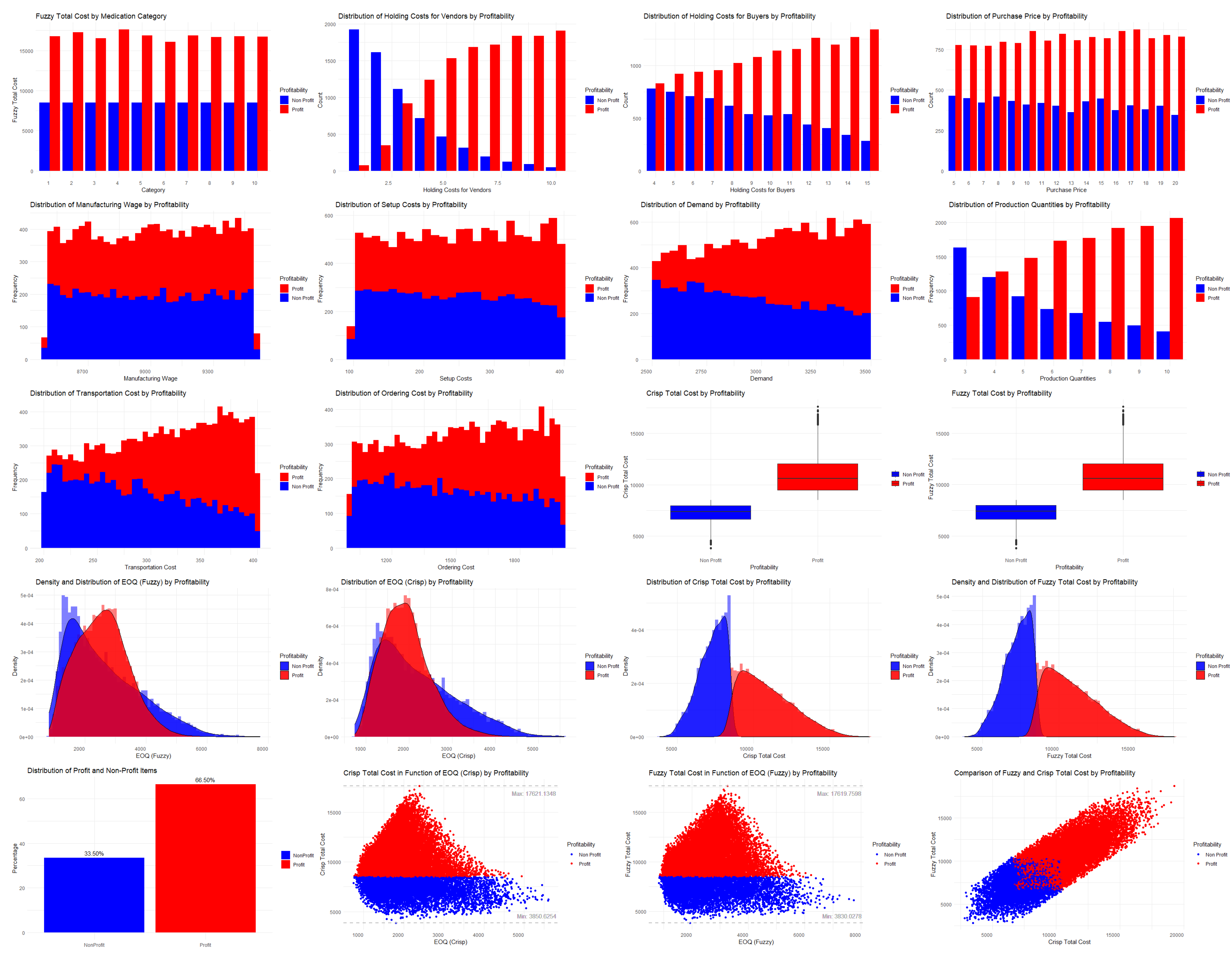
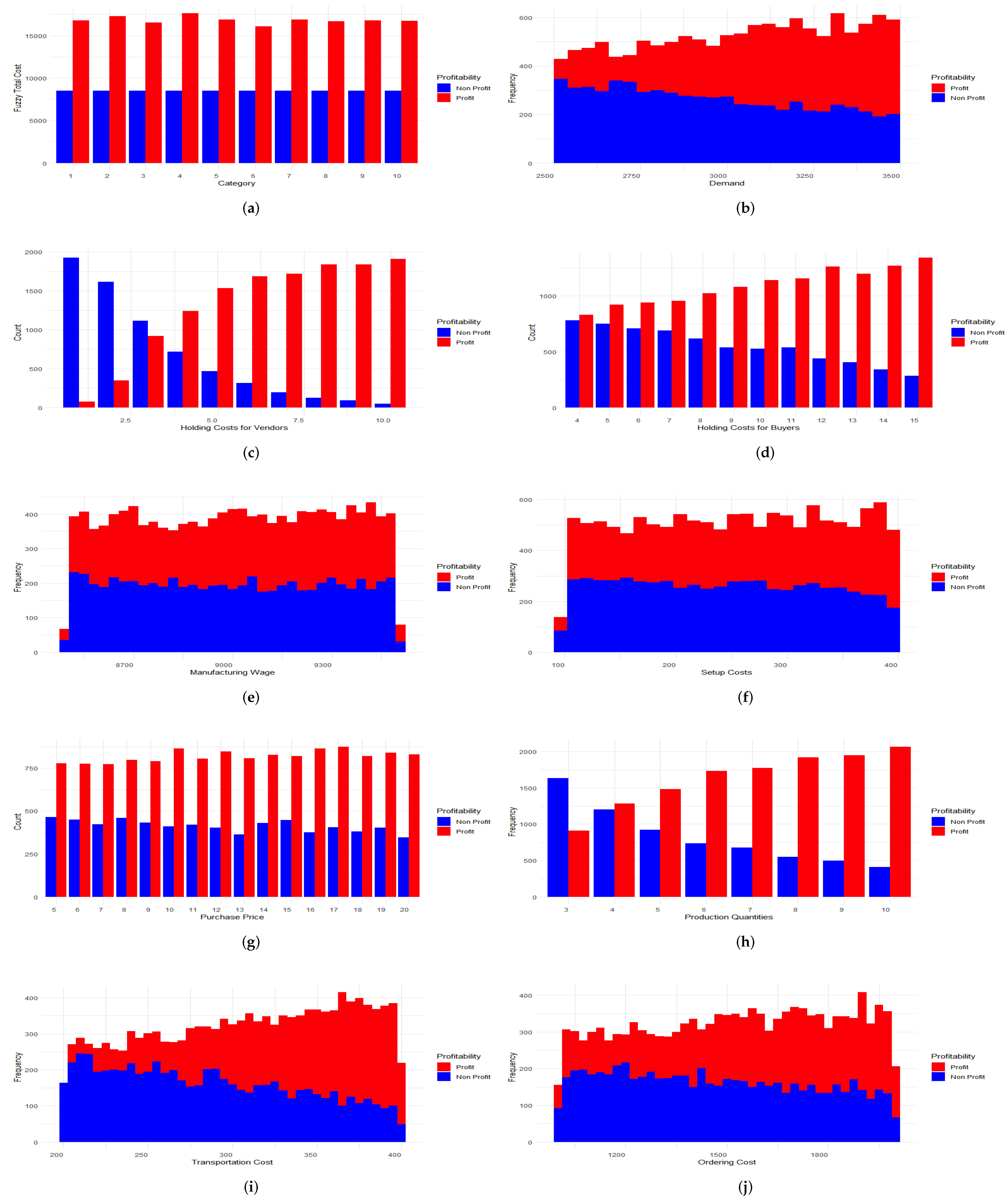
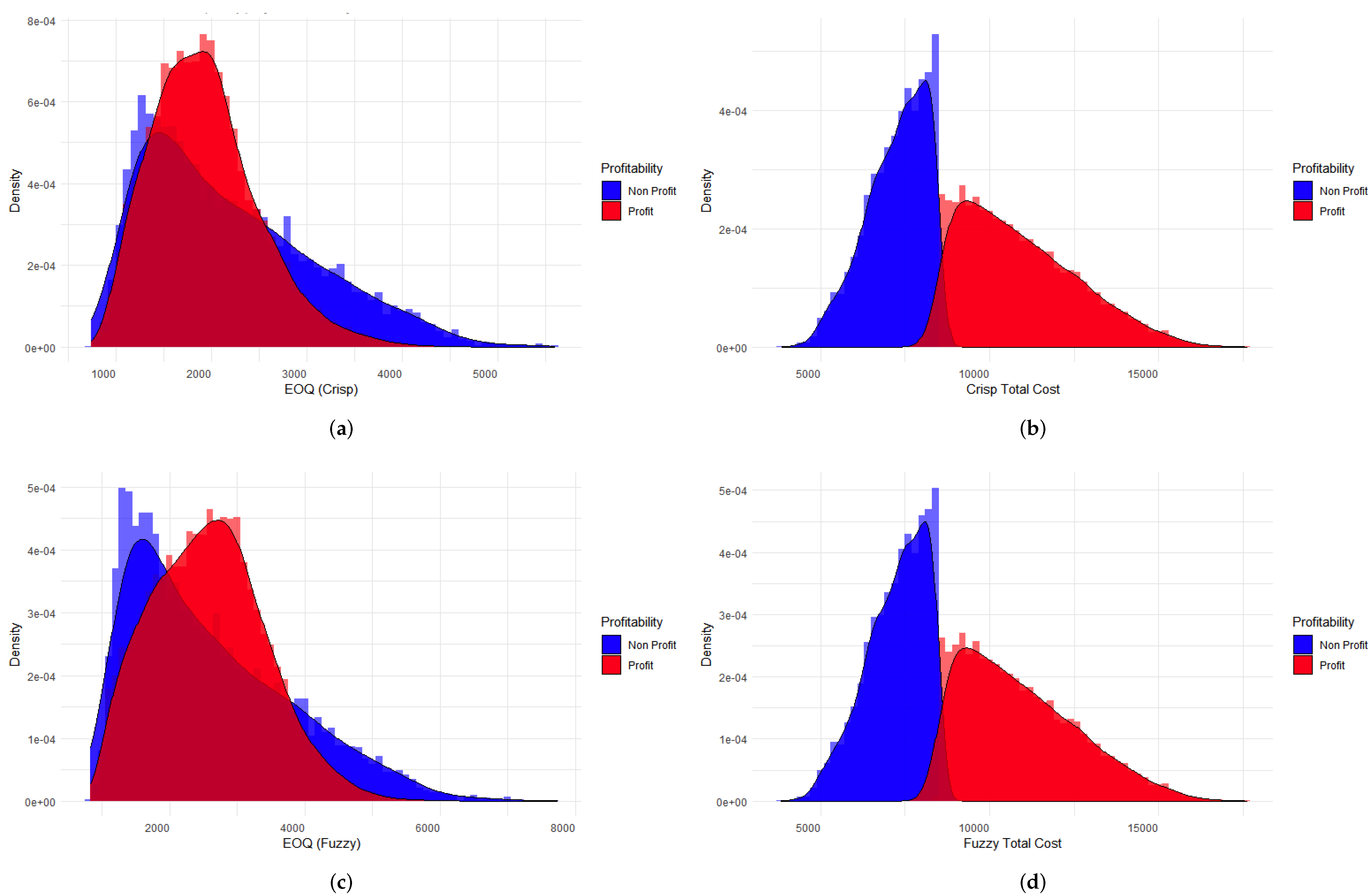
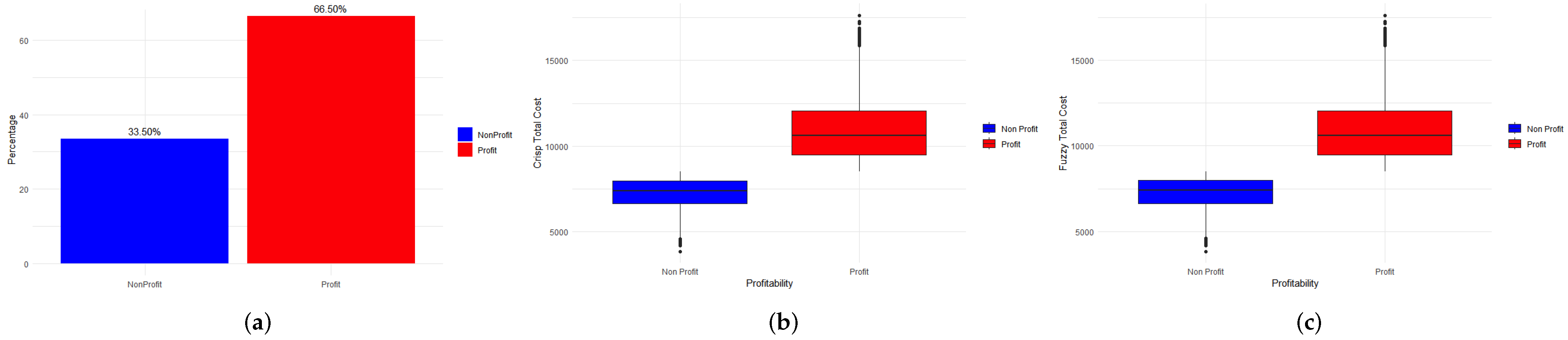
3.3. Visualization of the Results in the Weka Software

To complement our quantitative analysis, we next present a visual examination of drug profitability using the Weka software. The visualizations provide an intuitive understanding of the data, offering a different perspective that enhances the insights gained from the numerical analysis.

In the visual representations, we employ a consistent color scheme for clarity: blue signifies non-profit drugs, including newer market entries, less-commonly used drugs, or those for rarer ailments. Conversely, red depicts profitable drugs, which are more-established, widely used, and form the core of the pharmaceutical industry offerings.

To provide an overarching view of the factors influencing the profitability of pharmaceutical drugs, Figure 2 is introduced as a composite visualization, which is subsequently dissected into analyses for each parameter involved in the inventory TC.

Figure 3a illustrates a profitability analysis across ten different drug categories in the pharmaceutical industry, using a grouped bar-plot to depict fuzzy TC on the y-axis. The profitability of each category, expressed in monetary units per item, is depicted, distinguishing between profitable and non-profitable drugs. This figure aids in discerning market trends, such as identifying which drug categories are most lucrative and which may be oversaturated or less profitable. This analysis is valuable for manufacturers and dealers in making informed decisions regarding production and market strategies. The visualization encapsulates complex data in a straightforward manner, offering a clear depiction of the financial performance of different drug categories within the pharmaceutical market.

Figure 3a–j explore the financial dimensions influencing the profitability of pharmaceutical drugs, each from a distinct parameter. A multidimensional analysis helps to understand how each parameter contributes to the overall financial performance, showing a balance between supply chain efficiency and cost implications for both vendors and buyers.

Figure 3b–d analyze profitability in relation to key variables: demand (D), holding costs for vendors ($h_e$), and holding costs for buyers ($h_u$), respectively. Figure 3e,f,g,h show the impact of manufacturing-related costs on drug profitability, examining the effects of manufacturing wages (R), setup costs ($S_e$), purchase prices (P), and production quantities on the profit margins of pharmaceutical drugs. By breaking down these cost components, the figures offer insights into the cost structure of drug manufacturing and its influence on pricing and profitability strategies. Figure 3i,j focus on the logistical costs associated with pharmaceutical drugs, specifically examining how transportation costs (F) and ordering costs (U) affect profitability. This analysis helps to understand the impact of managing logistical expenses in the financial viability of drugs in the competitive pharmaceutical market.

Together, Figure 3a–j provide a comprehensive understanding of the various costs and factors that determine the profitability of pharmaceutical drugs. By highlighting the interplay between production, logistics, and market demand, they offer valuable insights for optimizing financial outcomes in pharmaceutical operations.

Figure 4a–d offer a comparison of the EOQ and TC across profit and non-profit scenarios for pharmaceutical drugs, employing both crisp and fuzzy logics. Figure 4a,c illustrate the empirical distribution of the EOQ (year) for profit and non-profit scenarios under crisp and fuzzy logics, respectively. Notably, the distributions differ significantly in shape, especially for profit scenarios. Both distributions exhibit positive skewness, yet the fuzzy logic approach reveals a more-flattened left tail of the distribution with a pronounced plateau, indicating a wider range of EOQ values considered optimal. For non-profit scenarios, the shape differences between crisp and fuzzy distributions are less pronounced. The range of EOQ values spans approximately from 740 to 5600 in the crisp case and from 820 to 7745 in the fuzzy case, suggesting that fuzzy logic accommodates a broader spectrum of optimal lot sizes.

Figure 4b,d focus on the TC associated with the EOQ under crisp and fuzzy logics, respectively. The resemblance in shape between the crisp and fuzzy cases is more evident, with both displaying slight positive skewness, indicating a common tendency towards lower TCs with a tail of higher-cost scenarios. However, the range of TCs is slightly greater in the crisp approach, reflecting a narrower focus on cost minimization that may not capture the full complexity of the pharmaceutical supply chain as effectively as the fuzzy approach. The comparison given in Figure 4 reveals the differences between crisp and fuzzy logics in modeling the EOQ and TCs. The fuzzy logic offers an inclusive and flexible model, accommodating a wider range of scenarios and demonstrating a capacity for handling the inherent uncertainties of the pharmaceutical industry supply chain more effectively.

While Figure 4 focuses on the inventory management aspect, Figure 5a shifts the perspective to a broader analysis of the market by presenting the number of profitable and non-profitable items across the studied pharmaceutical drugs. This figure provides a straightforward enumeration, showing the distribution of profitable versus non-profitable drugs within the market.

By using box-plots, Figure 5b,c provide a comparative analysis of the TC implications for drug profitability under deterministic (crisp) and fuzzy logic scenarios, respectively. While both box-plots visually suggest a similar distribution pattern across profit and non-profit categories, a closer inspection reveals subtle, yet impactful differences in the range of TCs captured by each model. The crisp model, utilizing fixed data points, offers a straightforward, albeit rigid, representation of cost dynamics. In contrast, the fuzzy logic model, by incorporating uncertain or imprecise data, slightly adjusts the cost boundaries, reflecting an understanding of market variability and its implications for drug profitability.

The observed variations between crisp and fuzzy analyses show the capability of fuzzy logic to accommodate the uncertainties of the pharmaceutical market, potentially offering a more-adaptable framework for cost management and strategic planning. By subtly shifting the cost parameters, the fuzzy model may reveal opportunities for cost optimization and risk management that a deterministic approach might overlook, emphasizing the importance of adopting flexible analytical strategies in the face of market complexities.

The comparison of the crisp and fuzzy analyses does not merely highlight their methodological differences, but also illustrates how the adoption of a fuzzy logic approach can subtly, yet significantly refine our understanding of TC implications in drug profitability. This refinement enhances decision-making processes, providing strategic insights that are critical for navigating the uncertainties inherent in the pharmaceutical industry.

Advancing our exploration into operational efficiency, Figure 6a,b examine the EOQ from deterministic and fuzzy perspectives, respectively. Figure 6a explores the EOQ in a crisp scenario, showing the application of deterministic models to optimize inventory management by aiming to minimize inventory TCs. Figure 6b displays the EOQ within a fuzzy logic framework, illustrating how embracing uncertainty and imprecision in inventory management strategies can potentially maximize the EOQ effectiveness.

The differential in TC variations between non-profit and profit categories under crisp and fuzzy models highlights the capacity of fuzzy logic to encompass a broader spectrum of market uncertainties. In particular, the fuzzy model adjusts the cost parameters more flexibly, reflecting a depth of market variability and its impact on profitability. This adjustment suggests that the fuzzy approach, by accounting for uncertainties more comprehensively, might offer a more-refined strategy for managing inventory costs and maximizing profitability. This indicates a strategic advantage in applying fuzzy logic for inventory management, allowing businesses to navigate the complexities of market conditions with greater agility and informed precision.

It is observed from the analyses presented in Figure 5 that employing fuzzy logic not only maximizes the EOQ, but also minimizes the TCs in comparison to the crisp values. This finding indicates that the fuzzy approach provides a more-effective framework for managing inventory and costs in the pharmaceutical industry, suggesting that the application of fuzzy logic enhances the decision-making process by better accommodating the complexities and uncertainties inherent in the market.

From our graphical analyses, we have offered a comprehensive view of how different mathematical models, particularly the fuzzy logic approach, contribute significantly to understanding and improving the profitability and operational efficiency of drug production and distribution in the pharmaceutical industry.

Figure 6c presents a comparison between the TCs associated with deterministic and fuzzy models in inventory management, as depicted through an elliptically shaped scatter plot with a positive slope. This visualization succinctly embodies the relationship between the cost outcomes of both modeling approaches, highlighting the variability and overlap in their cost efficiency when applied to pharmaceutical inventory management.

The elliptical shape of points suggests a correlation between the models in terms of cost implications, yet it also indicates the variability inherent in applying each method under different market conditions. This highlights the potential of fuzzy logic to offer competitive, if not superior, cost-minimization strategies compared to traditional crisp methods, particularly in scenarios characterized by uncertainty and complexity.

In summary, the present research affirms the value of integrating both deterministic and fuzzy logic models for sophisticated inventory management in the pharmaceutical supply chain. Figure 6c illustrates not merely the comparative costs, but also the broader applicability and effectiveness of these models in the pharmaceutical market. Our methodology facilitates the crafting of inventory management strategies that are not only more adaptable, but also cost-efficient, thereby enhancing the overall resilience and responsiveness of the supply chain.

By leveraging the strengths of both deterministic and fuzzy logic models, as demonstrated in Figure 6c, the present study provides compelling evidence for their combined utility in optimizing inventory management practices. Our methodology shows the importance of employing advanced analytical tools to better comprehend and address the challenges posed by the pharmaceutical supply chain, ultimately leading to more-strategic and -informed decision-making processes.

4. Discussion and Conclusions

This study presented an advancement in the field of inventory management within the pharmaceutical industry, particularly through the integration of fuzzy models, Kuhn–Tucker optimization techniques, and the naive Bayes classifier. The methodology proposed in this investigation has collectively addressed the complex dynamics of the pharmaceutical supply chain, offering novel insights into optimizing inventory management to enhance supply chain efficiency and, consequently, patient access to medications.

The application of pentagonal fuzzy numbers for production quantity representation highlighted our methodological innovation, catering to the inherent variability and uncertainty in production processes. The accuracy achieved by the naive Bayes classifier in a scenario classification (approximately 95.9%) showed the potential of combining machine learning with fuzzy logic to refine inventory strategies in dynamic environments.

The visual analysis conducted using the Weka software provided us with an intuitive understanding of the data, particularly in identifying profitable and non-profitable drug categories. The visualizations did not only make complex data comprehensible, but also revealed underlying market trends that are crucial for pharmaceutical manufacturers and dealers in making informed production and marketing decisions.

While our findings validated the effectiveness of the proposed integrated inventory model, it is important to acknowledge the limitations of our study. The current model application in scenarios involving multiple products and complex supply chain tiers remains unexplored. This limitation not only suggests the potential broad applicability of our model, but also reveals the need for future research to extend its capabilities.

The visualizations demonstrated the importance of considering various dimensions influencing drug profitability, which include demand, manufacturing, and logistical costs. Future research should aim to explore these dimensions further, utilizing more-sophisticated machine learning algorithms to enhance predictive accuracy and operational efficiency in the face of global health crises and fluctuating market demands.

The present study confirmed the efficacy of our integrated inventory model and highlighted the utility of advanced computational methods in improving decision-making for complex supply chain scenarios. Facing the dynamic challenges of epidemics and changing market demands, this research provided critical insights that can help to enhance the adaptability, resilience, and efficiency of supply chain operations in the pharmaceutical sector.

Future work should look to expand the model to include multi-product scenarios and incorporate epidemic modeling for a more-holistic approach to the supply chain management. Also, the digital era with the generation of big data [74] must be an aspect to be considered. These developments and additions are expected to significantly enhance both the theoretical framework and practical applications of the inventory management, offering new avenues for innovation within the pharmaceutical industry and related fields.

References

1. Goyal, S.K. An integrated inventory model for a single supplier-single customer problem. Int. J. Prod. Res. 1976, 15, 107–111. [Google Scholar] [CrossRef]
2. Goyal, S.K. Economic order quantity under conditions of permissible delay in payments. J. Oper. Res. Soc. 1985, 36, 335–338. [Google Scholar] [CrossRef]
3. Rojas, F.; Leiva, V.; Huerta, M.; Martin-Barreiro, C. Lot-size models with uncertain demand considering its skewness/kurtosis and stochastic programming applied to hospital pharmacy with sensor-related COVID-19 data. Sensors 2021, 21, 5198. [Google Scholar] [CrossRef]
4. Chand, S.; Ward, J. A note on economic order quantity under conditions of permissible delay in payments. J. Oper. Res. Soc. 1987, 38, 83–84. [Google Scholar]
5. Gupta, U.K. A comment on economic order quantity under conditions of permissible delay in payments. J. Oper. Res. Soc. 1988, 39, 322–323. [Google Scholar]
6. Chung, K.J. A theorem on the determination of economic order quantity under conditions of permissible delay in payments. Comput. Oper. Res. 1998, 25, 49–52. [Google Scholar] [CrossRef]
7. Chung, K.J.; Huang, C.K. An ordering policy with allowable shortage and permissible delay in payments. Appl. Math. Model. 2009, 33, 2518–2525. [Google Scholar] [CrossRef]
8. Chang, H.J.; Hung, C.H.; Dye, C.Y. An inventory model for deteriorating item with linear trend demand under the condition of permissible delay in payments. Prod. Plan. Control. 2001, 12, 274–282. [Google Scholar] [CrossRef]
9. Rojas, F.; Leiva, V.; Wanke, P.; Marchant, C. Optimization of contribution margins in food services by modeling independent component demand. Colomb. J. Stat. 2015, 38, 1–30. [Google Scholar] [CrossRef]
10. Teng, T.J. On the economic order quantity under conditions of permissible delay in payments. J. Oper. Res. Soc. 2002, 53, 915–918. [Google Scholar] [CrossRef]
11. Huang, H.; Shin, S.W. Retailer’s pricing and lot sizing for exponentially deteriorating products under the condition of permissible delay in payments. Comput. Oper. Res. 1997, 24, 539–547. [Google Scholar]
12. Huang, Y.F. Optimal retailer’s ordering policies in the EOQ model under trade credit financing. J. Res. Soc. 2003, 54, 1011–1015. [Google Scholar] [CrossRef]
13. Wanke, P.; Ewbank, H.; Leiva, V.; Rojas, F. Inventory management for new products with triangularly distributed demand and lead-time. Comput. Oper. Res. 2016, 69, 97–108. [Google Scholar] [CrossRef]
14. Park, K.S. Fuzzy set theoretic interpretation of economic order quantity. IEEE Trans. Syst. Man, Cybern. Smc 1987, 17, 1082–1084. [Google Scholar] [CrossRef]
15. Rojas, F.; Wanke, P.; Leiva, V.; Huerta, M.; Martin-Barreiro, C. Modeling inventory cost savings and supply chain success factors: A hybrid robust compromise multi-criteria approach. Mathematics 2022, 10, 2911. [Google Scholar] [CrossRef]
16. Rojas, F.; Leiva, V.; Wanke, P.; Lillo, C.; Pascual, J. Modeling lot-size with time-dependent demand based on stochastic programming and case study of drug supply in Chile. PLoS ONE 2019, 14, e0212768. [Google Scholar] [CrossRef] [PubMed]
17. Huerta, M.; Leiva, V.; Rojas, F.; Wanke, P.; Cabezas, X. A methodology for consolidation effects of inventory management with serially dependent random demand. Processes 2023, 11, 2008. [Google Scholar] [CrossRef]
18. Palanivelu, K.U.B.; Leiva, V.; Dhandapani, P.B.; Castro, C. On fuzzy and crisp solutions of a novel fractional pandemic model. Fractal Fract. 2023, 7, 528. [Google Scholar]
19. Rangasamy, M.; Alessa, N.; Dhandapani, P.B.; Loganathan, K. Dynamics of a novel IVRD pandemic model of a large population over a long time with efficient numerical methods. Symmetry 2022, 14, 1919. [Google Scholar] [CrossRef]
20. Kalpana, U.; Balaganesan, P.; Renuka, J.; Dumitru, B.; Dhandapani, P.B. On the decomposition and analysis of novel simultaneous SEIQR epidemic model. AIMS Math. 2023, 10, 5918–5933. [Google Scholar]
21. Sebatjane, M.; Adetunji, O. A four-echelon supply chain inventory model for growing items with imperfect quality and errors in quality inspection. Ann. Oper. Res. 2024, in press. [CrossRef]
22. Alamri, O.A. Sustainable supply chain model for defective growing items (fishery) with trade credit policy and fuzzy learning effect. Axioms 2023, 12, 436. [Google Scholar] [CrossRef]
23. Alamri, O.A.; Jayaswal, M.K.; Khan, F.A.; Mittal, M. An EOQ Model with Carbon Emissions and Inflation for Deteriorating Imperfect Quality Items under Learning Effect. Sustainability 2022, 14, 1365. [Google Scholar] [CrossRef]
24. Chang, H.C. An application of fuzzy sets to the EOQ model with imperfect quality items. Comput. Oper. Res. 2004, 31, 2079–2092. [Google Scholar] [CrossRef]
25. Rani, S.; Ali, R.; Agarwal, A. Fuzzy inventory model for new and refurbished deteriorating items with cannibalization in green supply chain. Int. J. Syst. Sci. Oper. Logist. 2022, 9, 22–38. [Google Scholar]
26. Wee, H.M.; Yu, J.; Chen, M.C. Optimum inventory model for items with imperfect quality and shortage backordering. Omega 2007, 35, 7–11. [Google Scholar] [CrossRef]
27. Rajeswari, S.; Sugapriya, C.; Nagarajan, D.; Kavikumar, J. Optimization in fuzzy economic order quantity model involving pentagonal fuzzy parameter. Int. J. Fuzzy Syst. 2022, 24, 44–56. [Google Scholar] [CrossRef]
28. Jayaswal, M.K.; Mittal, M.; Alamri, O.A.; Khan, F.A. Learning EOQ Model with Trade-Credit Financing Policy for Imperfect Quality Items under Cloudy Fuzzy Environment. Mathematics 2022, 10, 246. [Google Scholar] [CrossRef]
29. Banerjee, A. A joint economic lot size model for purchase and vendor. Decis. Sci. 1986, 17, 292–311. [Google Scholar] [CrossRef]
30. Chen, S.K. Operations on fuzzy numbers with function principle. Tamkang J. Mang. Sci. 1985, 6, 13–26. [Google Scholar]
31. Zhao, H.; Jiang, Y.; Yang, Y. Robust and Sparse Portfolio: Optimization Models and Algorithms. Mathematics 2023, 11, 4925. [Google Scholar] [CrossRef]
32. Kotz, S.; Leiva, V.; Sanhueza, A. Two new mixture models related to the inverse Gaussian distribution. Methodol. Comput. Appl. Probab. 2010, 12, 199–212. [Google Scholar] [CrossRef]
33. Kalaiarasi, K.; Sumathi, M.; Mary Henrietta, H. Optimizing EOQ using geometric programming with varying fuzzy numbers by applying Python. J. Crit. Rev. 2020, 7, 596–603. [Google Scholar]
34. Kalaiarasi, K.; Soundaria, R.; Kausar, N.; Agarwal, P.; Aydi, H.; Alsamir, H. Optimization of the average monthly cost of an EOQ inventory model for deteriorating items in machine learning using Python. Therm. Sci. 2021, 2, S347–S358. [Google Scholar] [CrossRef]
35. Chen, S.H.; Hsieh, C.H. Optimization of fuzzy inventory models. In Proceedings of the IEEE SMC99 Conference, Tokyo, Japan, 12–15 October 1999; Volume 1, pp. 240–244. [Google Scholar]
36. Dong, Y.; Xu, K. A supply chain model of vendor managed inventory. Transp. Res. Part Logist. Transp. Rev. 2002, 38, 75–95. [Google Scholar] [CrossRef]
37. Marquès, G.; Thierry, C.; Lamothe, J.; Gourc, D. A review of vendor managed inventory (VMI): From concept to processes. Prod. Plan. Control. 2010, 21, 547–561. [Google Scholar] [CrossRef]
38. Lotfi, R.; MohajerAnsari, P.; Nevisi, M.M.S.; Afshar, M.; Davoodi, S.M.R.; Ali, S.S. A viable supply chain by considering vendor-managed-inventory with a consignment stock policy and learning approach. Results Eng. 2024, 21, 101609. [Google Scholar] [CrossRef]
39. Silva, R.; Tarigan, Z.; Siagian, H. The influence of supplier competency on business performance through supplier integration, vendor-managed inventory, and supply chain collaboration in Fuel Station: An evidence from Timor Leste. Uncertain Supply Chain. Manag. 2024, 12, 207–220. [Google Scholar] [CrossRef]
40. Rahman, M.Z.; Akbar, M.A.; Leiva, V.; Tahir, A.; Riaz, M.T.; Martin-Barreiro, C. An intelligent health monitoring and diagnosis system based on the internet of things and fuzzy logic for cardiac arrhythmia COVID-19 patients. Comput. Biol. Med. 2023, 154, 106583. [Google Scholar] [CrossRef]
41. Rangasamy, M.; Chesneau, C.; Martin-Barreiro, C.; Leiva, V. On a novel dynamics of SEIR epidemic models with a potential application to COVID-19. Symmetry 2022, 14, 1436. [Google Scholar] [CrossRef]
42. Rahman, M.Z.U.; Akbar, M.A.; Leiva, V.; Martin-Barreiro, C.; Imran, M.; Riaz, M.T.; Castro, C. An IoT-fuzzy intelligent approach for holistic management of COVID-19 patients. Heliyon 2024, 10, e22454. [Google Scholar] [CrossRef] [PubMed]
43. Taylan, O.; Alkabaa, A.S.; Alqabbaa, H.S.; Pamukcu, E.; Leiva, V. Early prediction in classification of cardiovascular diseases with machine learning, neuro-fuzzy and statistical methods. Biology 2023, 12, 1179. [Google Scholar] [CrossRef] [PubMed]
44. Kuppusamy, V.; Shanmugasundaram, M.; Dhandapani, P.B.; Martin-Barreiro, C.; Cabezas, X.; Leiva, V.; Castro, C. Addressing a decision problem through a bipolar Pythagorean fuzzy approach: A novel methodology with application in digital marketing. Heliyon 2024, 10, e23991. [Google Scholar] [CrossRef]
45. Mittal, M.; Jain, V.; Pandey, J.T.; Jain, M.; Dem, H. Optimizing Inventory Management: A Comprehensive Analysis of Models Integrating Diverse Fuzzy Demand Functions. Mathematics 2024, 12, 70. [Google Scholar] [CrossRef]
46. Alshammari, O.; Kchaou, M.; Jerbi, H.; Ben Aoun, S.; Leiva, V. A fuzzy design for a sliding mode observer-based control scheme of Takagi-Sugeno Markov jump systems under imperfect premise matching with bio-economic and industrial applications. Mathematics 2022, 10, 3309. [Google Scholar] [CrossRef]
47. Zadeh, L.A. Fuzzy sets. Inf. Control. 1965, 8, 338–353. [Google Scholar] [CrossRef]
48. Klir, G.J.; Yuan, B. Fuzzy Sets and Fuzzy Logic: Theory and Applications; Prentice Hall: Hoboken, NJ, USA, 1995. [Google Scholar]
49. Zimmermann, H.J. Fuzzy Set Theory—and Its Applications; Kluwer Academic Publishers: Boston, MA, USA, 2001. [Google Scholar]
50. Dubois, D.; Prade, H. Fuzzy Sets and Systems: Theory and Applications; Academic Press: Cambridge, MA, USA, 1980. [Google Scholar]
51. Nguyen, H.T.; Walker, E.A. A First Course in Fuzzy Logic; CRC Press: Boca Raton, FL, USA, 1996. [Google Scholar]
52. Ghaznavi, M.; Soleimani, F.; Hoseinpoor, N. Parametric Analysis in Fuzzy Number Linear Programming Problems. Int. J. Fuzzy Syst. 2016, 18, 463–477. [Google Scholar] [CrossRef]
53. Kaufmann, A.; Gupta, M.M. Introduction to Fuzzy Arithmetic Theory and Applications; Van Nostrand Reinhold: New York, NY, USA, 1985. [Google Scholar]
54. Khan, I.U.; Ahmad, T.; Maan, N. A simplified novel technique for solving fully fuzzy linear programming problems. J. Optim. Theory Appl. 2013, 159, 536–546. [Google Scholar] [CrossRef]
55. Mordeson, J.N.; Nair, P.S. Fuzzy Mathematics: An Introduction for Engineers and Scientists; Physica-Verlag: Heidelberg, Germany, 2001. [Google Scholar]
56. Bede, B. The Mathematics of Fuzzy Sets and Fuzzy Logic; Springer: Berlin, Germany, 2007. [Google Scholar]
57. Panda, A.; Pal, M. A study on pentagonal fuzzy number and its corresponding matrices. Pac. Sci. Rev. Humanit. Soc. Sci. 2015, 1, 131–139. [Google Scholar] [CrossRef]
58. Mondal, S.P.; Mandal, M. Pentagonal fuzzy number, its properties and application in fuzzy equation. Future Comput. Inform. J. 2017, 2, 110–117. [Google Scholar] [CrossRef]
59. Taha, H.A. Operations Research; Prentice-Hall: Englewood Cliffs, NJ, USA, 1997. [Google Scholar]
60. Bazaraa, M.S.; Sherali, H.D.; Shetty, C.M. Nonlinear Programming: Theory and Algorithms; Wiley-Interscience: Hoboken, NJ, USA, 2006. [Google Scholar]
61. Boyd, S.; Vandenberghe, L. Convex Optimization; Cambridge University Press: Cambridge, UK, 2004. [Google Scholar]
62. Luenberger, D.G. Optimization by Vector Space Methods; John Wiley & Sons: New York, NY, USA, 1969. [Google Scholar]
63. Hillier, F.S.; Lieberman, G.J. Introduction to Operations Research; McGraw-Hill: New York, NY, USA, 2001. [Google Scholar]
64. Nagar, H.; Surana, P. Fuzzy inventory model for deteriorating item by using signed distance method in which inventory parameters are treated as Pfn. Indian J. Appl. Res. 2015, 7, 628–634. [Google Scholar]
65. Atanassov, K.T. Fuzzy Sets and Their Applications to Cognitive and Decision Processes; Academic Press: New York, NY, USA, 1976. [Google Scholar]
66. Kacprzyk, J.; Fedrizzi, M. Fuzzy Sets, Decision Making, and Expert Systems; Kluwer Academic Publishers: Boston, MA, USA, 1986. [Google Scholar]
67. Taylor, B.W. Introduction to Management Science; Pearson: New York, NY, USA, 2019. [Google Scholar]
68. Nahmias, S. Production and Operations Analysis; McGraw-Hill/Irwin: New York, NY, USA, 2009. [Google Scholar]
69. Silver, E.A.; Pyke, D.F.; Peterson, R. Inventory Management and Production Planning and Scheduling; John Wiley & Sons: New York, NY, USA, 1998. [Google Scholar]
70. Ritha, W.; Kalaiarasi, R.; Jun, Y.B. Optimization of fuzzy integrated vendor–buyer inventory models. Ann. Fuzzy Math. Inform. 2011, 2, 239–257. [Google Scholar]
71. Kausar, N.; Munir, M.; Agarwal, P.; Kalaiarasi, K. The characterization of fuzzy and anti fuzzy Ideals in AG-groupoid. Thai J. Math. 2022, 20, 653–667. [Google Scholar]
72. Kalaiarasi, K.; Henrietta, H.M.; Sumathi, M. Determining the efficient optimal order quantity for an Inventory model with varying fuzzy components. J. Algebr. Stat. 2022, 6, 653–667. [Google Scholar]
73. Kalaiarasi, K.; Nasreen Kausar, P.; Kousar, S.; Pamucar, D.; Ide, N.A.D. Economic order quantity model-based optimized fuzzy nonlinear dynamic mathematical schemes. Comput. Intell. Neurosci. 2022, 2022, 3881265. [Google Scholar]
74. Aykroyd, R.G.; Leiva, V.; Ruggeri, F. Recent developments of control charts, identification of big data sources and future trends of current research. Technol. Forecast. Soc. Chang. 2019, 144, 221–232. [Google Scholar] [CrossRef]
75. Kononenko, I.; Bratko, I. Information-based evaluation criterion for classifier’s performance. Mach. Learn. 1991, 6, 67–80. [Google Scholar] [CrossRef]
Figure 1. Flowchart of the proposed process.
Mathematics 12 00819 g001
Figure 2. Plots of pharmaceutical drug profitability: integrating profit and non-profit analyses across indicated cost or demand parameter.
Mathematics 12 00819 g002
Figure 3. Bar-plots—(a,c,d,g,h)—and histograms with ’frequency’ in the y-axis being the absolute frequency of the data—(b,e,f,i,j)—of profit/non-profit in pharmaceutical drugs for: (a) category; (b) demand, D; (c) holding cost for vendors, h e ; (d) holding cost for buyers, h u ; (e) manufacturing wage, R; (f) setup cost, S e ; (g) purchase price, P; (h) quantity; (i) transportation cost, F; and (j) ordering cost of the drug, U.
Mathematics 12 00819 g003
Figure 4. Histograms with kernel density and ’density’ in the y-axis being the relative frequency of the data of profit/non-profit in pharmaceutical drugs by the drug lot size, J say, for (a) crisp EOQ; (b) crisp TC, (c) fuzzy EOQ; and (d) fuzzy TC.
Mathematics 12 00819 g004
Figure 5. (a) Bar-plot of the number of profit and non-profit items; (b) crisp TC box-plot by drug profitability; and (c) fuzzy TC box-plot by drug profitability.
Mathematics 12 00819 g005
Figure 6. Scatter-plots of (a) crisp EOQ versus crisp TC; (b) fuzzy EOQ versus fuzzy TC; and (c) crisp TC versus fuzzy TC.
Mathematics 12 00819 g006