Abstract
In this paper, the derivation of a concise closed form for the gravitational field of a polyhedron is presented. This formula forms the basis of the algorithm for calculating the gravitational field of an arbitrary shape body with high accuracy. Based on this algorithm, a method for gravity data inversion (creating density models of the Earth’s crust) has been developed. The algorithm can accept either regular or irregular polyhedron discretization for density model creation. The models are approximated with dense irregular grids, elements of which are polyhedrons. When performing gravity data inversion, we face three problems: topography with large amplitude, the sphericity of the planet, and a long computation time because of the large amount of data. In our previous works, we have already considered those problems separately but without explaining the details of the computation of the closed-form solution for a polyhedron. In this paper, we present for the first time a performance-effective numerical method for the inversion of gravity data based on topography. The method is based on closed-form expression for the gravity field of a spherical density model of the Earth’s crust with the upper topography layer, and provides great accuracy and speed of calculation. There are no restrictions on the model’s geometry or gravity data grid. As a case study, a spherical density model of the Earth’s crust of the Urals is created.
Keywords:
gravity data inversion; spherical density model of Earth’s crust with the upper topography layer; gravitational field of a polyhedron MSC:
86A22; 86-10; 86-08
1. Introduction
The initial data used for constructing density models of the Earth’s crust are the measured values of gravity anomalies. One of the stages of observed data preprocessing is the correction for topography. It consists of calculating the gravitational effect of masses (at the observation point) lying above some reference surface, for example, the Earth’s ellipsoid. The “classical” approximation of this stage (for a “flat” model) can be called the calculation of the correction for the influence of the intermediate plane-parallel layer, which is included in the Bouguer correction [1]. The values of errors in the field (arising when introducing a correction for topography) significantly exceed the resolution of modern gravimeters [2]. A number of authors have studied the problem of correction for the Earth’s spherical shape in the results of gravimetric data inversion for the creation of density models. Heck and Seitz [3] suggested replacing the elements of spherical models by rectangular prisms or, for the distant observation points, by the selected point masses. Wild-Pfeiffer et al. [4] and Uieda et al. [5] used the Gauss–Legendre cubature formulas for calculating the gravity field of a tesseroid. They also implemented a parallel algorithm based on OpenMP technologies for computing the gravity field of large composite models at an arbitrary set of points. Bouman et al. [6] studied the possibility of constructing regional spherical density models using highly accurate gravity satellite measurements. The main purpose of this kind of investigation is to optimize the algorithms and time consumption for computing the spheroidal bodies’ fields, and their application for creating density models taking the curvature of the real Earth into account.
During observed gravity data preprocessing, researchers use various methods to recalculate the data from topography to a reference surface (plane, surface of the Earth ellipsoid). To perform this stage without a loss of accuracy, we need to have the density values in the domain between the measurement surface and the reference surface. These values are unknown and, in fact, the final goal of solving the initial problem is to discover them. Usually, researchers use speculative or heuristic medium density values. To obtain a more accurate result of the inversion, we need to use gravity data measured directly on the topography, without recalculation to an auxiliary reference surface. In [2], the authors proposed the algorithm of forward problem solving (parallelized for graphics processing units—GPUs) for real topography using the irregular grids of the density model and field. The algorithm is based on the concise closed form of the gravitational field of a polyhedron. The algorithm has high speed and accuracy, and therefore, on its basis, it is possible to develop a method for interpreting gravitational data based on topography. As result of gravity data inversion, we will create a spherical model which has the surface of the topography as the upper boundary. This approach will significantly improve the accuracy of determining the parameters of the model.
Considering similar approaches to solving the inverse problem, it is necessary to note paper [7], the authors of which also take into account topography. The paper describes in detail synthetic and real examples of density model creation using the observed gravity data and presents the results of calculations using various weighting functions. An irregular grid is used to increase its step by the depth. This may allow us to obtain good resolution in the topography layers. It is highlighted that topography significantly influences the measured (calculated) gravity field. Unfortunately, the article does not describe in detail the method used to solve the direct and inverse problems, or the optimization methods, and it does not provide details of the software and hardware. The presented models have less than 106 partitioning elements, which is not enough for regional-scale models of adequate resolution. Since the region under consideration has a small area, the authors did not need to take into account the sphericity of the planet. A regular grid is used on the plane, and not on the topography. In our article, we will try to address these issues in more detail.
In [8], the authors performed gravitational modeling of near-surface lunar objects, including topography. To calculate the gravitational integral in spherical coordinates, the Gauss–Legendre quadrature method was used. The authors were unable to obtain a detailed model due to the high computational complexity of the method under consideration; however, the paper presents estimations of the average structural density in the crust, mantle, and core. The computational optimizations in our method allow us to overcome this limitation.
2. The Forward Gravity Problem
Let us define what we mean by a spherical three-dimensional density model with a depth H. Let the upper boundary S of this model (on the side of the Earth–air surface) be a part of the rotational ellipsoid; all of the points, located within depth H along the internal normal to S, belong to the model. In this domain , the density distribution is specified, , where .
The vertical component of the gravity field that is produced by the domain D in the external point is determined by the following integral:
where is the gravitational constant, is the volume element of integration, is the external normal to S in the orthogonal projection of point on S (i.e., coincides with the normal to the ellipsoid’s surface in the case of a spherical model), and and are radii-vectors of points and , respectively. Note that Formula (1) describes the projection of the total vector of the gravitational field strength onto the unit vector , i.e., is the part of total field in the direction of .
Calculating the Field of a Spherical Model Based on the Topography
Let us consider a spherical density model in 3D space down to depth H with an upper topography layer. The model’s “upper” boundary T (Earth–air interface) is the topography surface (height map) relative to the surface S of an ellipsoid of revolution (for example, the World Geodetic System 1984 (WGS84) [9] reference ellipsoid) along its external normal. All points located at a distance of no more than H, along the inner normal to S, and no more than , along the outer normal, belong to the model, where is the elevation of T over S, is the latitude, and is the longitude associated with the ellipsoid. In the described domain , the density distribution is defined as , where .
Let us choose some discretization of and approximate the volume of an element of the partition by a polyhedron , obtaining an approximated model. Now, we can apply the previously proposed [10] algorithm to solve the forward gravity problem. Let us represent the basic steps of the algorithm and for the first time present the derivation of the closed-form formula for the gravitational field of a polyhedron.
Let the density of each be uniform and equal to . The field for the model D at the point Q can be calculated through the sum of the fields of each discretization element:
where is the field of the element with unit density at the point Q up to the coefficient .
The integral (1) for the field cannot be expressed in a closed form. It is also difficult to calculate the integral numerically with cubature formulas, since the boundaries of can have complex descriptions. It would require first or second order formulas with a large number of nodes and a large computing time in order to achieve acceptable accuracy. This is why we calculate the integral (1) not for , but for the approximating polyhedron . We denote the set of faces as , then we calculate the following:
Next, we convert the volume integral into the surface integral, applying the divergence theorem to (2), as follows:
The surface integral can be split into a sum of integrals for each of the faces of . Note that the external normal is constant at every point of an integration face:
where is the external normal to the face .
Next, we find a closed-form expression for the integral over a triangle. In fact, this integral is the gravity potential of the triangle plate with a density equal to . Let us denote () as radius vectors of the triangle vertices ; is the point of field calculation; ; ; is the normal to the triangle with the length equal to its double surface area; is the unit normal to the triangle; ; is the (signed) distance from the point to the triangle surface. From this, we can denote the following:
where are radii vectors of the vertices of the triangle. Let us introduce new parameters and as follows: , , , and . Then, we have and the following formula:
In expression , we select a full square by variable : , where . Note that the vector product is independent of , and the scalar product is a linear function of . Thus, the integral is the table integral . Therefore, we have the following:
Similarly, in both terms of the resulting integrand in , we select a full square by variable : ; . Thus, both terms in Formula (3) are reduced to the following integral:
After partial integration, we have the following:
By multiplying the numerator and denominator in the last two terms by , we have the following:
As one can see, the denominators of the integrands contain the expressions and . If one makes a change to the variable, after which there is no linear term left in the quadratic functions, it is possible to reduce the integrals to tabular ones. By making a general substitution in the expressions and and equating the coefficients of t in the numerator to 0, we can obtain the unknown parameters: ; . Then, we obtain an explicit substitution as follows: , , , , , and . Using Formula (5), we can make substitutions and partial integrations with the original integral (4) as follows:
Further, let us suppose that . We can find the explicit form of the second integral in Formula (6):
Let us find the explicit form of the first integral in Formula (6):
According to [11] (1.2.45.2), we have the following:
By making the substitution , , and , and according to [11] (1.2.44.6), we have the following:
For the third integral in Formula (8), according to [11] (1.2.46.11, 1.2.46.12), we have the following:
By substituting (9)–(11) into (8), then (7) and (8) into (6), and performing the inverse substitution and a number of transformations for simplicity, we obtain the following:
where , , , and .
Using Formula (12), we obtain for the following representation:
Using formulas for adding arctangents and a formula for the value of the solid angle at which an arbitrary triangle is visible from an observation point in space [12], and performing transformations, we obtain the final formula as follows:
where , , , and ; is the unit normal to the triangle, is a distance from the observed point to the triangle surface, and is the solid angle at which an arbitrary triangle is visible from an observation point.
We suggest a parallel algorithm to calculate the gravitational field of spherical models using the derived formulas. Based on the NVidia® CUDA® and AMD ROCm™ libraries, a software tool has been developed using multi-threaded data processing technologies on GPU, which allows us to calculate the gravitational field values of the spherical models on an arbitrarily specified grid. The computation in this approach can be conducted on several GPU simultaneously, which significantly speeds up the program. The source codes of the program, distribution kit, test model, and user instructions are publicly available at https://github.com/AlexIII/GRAFEN (accessed on 10 March 2024) under a free MIT license. The convergence, speed, and errors of computing the gravity field by using the proposed method were tested by comparison with the five-point Gauss–Legendre (GL) numerical integration method [10] for various configurations of partitions of the “ellipsoidal” model of the Earth’s crust. The testing showed that the increase in computation speed by the proposed method is tens of times (compared to the Gauss–Legendre method), with an equivalent error rate. Table 1 illustrates the difference between the gravity field values calculated by the proposed method for the 1335 × 968 partition and those calculated by the GL method for different partitions.

Table 1.
Comparison of the tesseroid field values calculated for different partitions by the GL method and the suggested methods. is the field for the partition indicated for the given column in the GL method, is the field for the smaller partition (with half the number of elements in x and y) in the GL method; is the field calculated by the method suggested in this study for a smaller partition of 1335 × 968.
3. Inverse Problem of Gravimetry
This paper considers a discrete formulation of the three-dimensional inverse problem of gravimetry (the process of calculating density values from the observed field). The observed field is specified at a certain set of points on the topography. The density distribution is sought in the form of a piecewise constant function on a given grid. In this case, the inverse problem is reduced to solving a system of linear equations:
where A is the operator of the direct problem (matrix), x is the vector of density values of the model’s partition elements, and f is the vector of values of the discretized field .
The three-dimensional inverse problem of gravimetry for the density distribution restoration of the given observed field is in this general case ill posed, so in order to solve it, it is necessary to use regularization methods. We will seek a regularized solution to (13) as a minimum of the following functional:
This problem is equivalent to finding a solution to the following operator equation (least squares method with regularization):
where E is the identity matrix. Formula (14) can be solved efficiently (in terms of computational resources) by using the conjugate gradient method [13]. The iterative process is described as follows:
Here, k is the iteration number, , and . Without the loss of generality, the initial guess is always chosen to be zero (x0 = 0), since the gravitational effect of any non-zero initial guess model can always be subtracted from the measured field. The termination criterion is over two consecutive iterations. For more precise control over the distribution of features in the solution, we will use the parameter λ as a depth variable: , or for a discrete case (the vector of weighting coefficients along the “horizontal” layers of the model). The choice of coefficients depends on the specific problem under consideration; they are selected in such a way that the characteristics of the resulting solution correspond to the available a priori data (for example, the average density distribution over depth).
The key point is the availability of a computationally efficient software for parallel implementation of the algorithm to solve the forward problem. It allows one to search for a solution to the inverse problem for high-resolution density models (with the number of partition elements of the order of 108) within an acceptable time. Previously, the authors developed such a software implementation based on the original algorithm [10] for an ellipsoidal model of a section of the Earth’s crust and demonstrated its speed and accuracy in comparison to Gauss–Legendre cubature formulas. Then, the algorithm was generalized to solve a forward problem on the topography (given by a height map) [2]. Next, the described inverse problem algorithm was tested on synthetic models, which made it possible to evaluate characteristics such as the convergence rate, the calculation time, and the dependence of the solution morphology on the values of the tuning parameters. In this work, we will consider an example of solving the inverse problem (using a similar partition grid) for a practical model of the Urals region.
4. Case Study
Digital model XGM2019e_2159 of the gravitational field of the study area (60°–68° N 48°–72° E) was obtained from the International Center for Global Earth Models (ICGEM) online resource [14]. The selected data representation, a “gravity disturbance”, is an array of values of the vertical derivative of the gravitational potential on the topography minus the value of the vertical derivative of the normal field potential at the same point. From this representation, two input files are obtained: a map of relief heights and the values of the vertical component of the gradient of the gravitational field potential on a uniform degree grid. At the stage of preparing the input data, the grid is converted from a geodetic coordinate system to Gauss–Kruger coordinates (using the WGS84 datum), as well as being recalculated to a grid uniform in distance. This allows us to eliminate the problem of irregular (in terms of distance) partition density and the associated irregular error in the approximation of the model geometry.
When solving an inverse problem, one of the key factors is the presence of an initial approximation model containing a priori data on the density distribution. Such a model must include all of the required geological features, since we will be looking for a solution that differs minimally from the real density values in the quadratic metric. For the territory under consideration, part of the initial approximation model, located “below” the surface of the reference ellipsoid, was built based on the existing Deep Seismic Sounding (DSS) profiles according to the method described in [2]. The layer of relief-forming rocks (the area “above” the surface of the reference ellipsoid) in the initial approximation model was filled with a constant density of 2.67 g/cm3. The number of partition elements of the resulting model turned out to be 358 × 261 × 81, about 107; approximate dimensions of the partition element in the layers below the reference surface were 4 km × 4 km × 1 km. The gravitational field was calculated for the model and subtracted from the observed field. The result of this subtraction is the “residual” field (see Figure 1); its values are taken as a vector in Formula (14), and a solution is searched for it to obtain density values. This solution is subsequently added to the zero-approximation model. Table 2 shows the main characteristics of the described gravitational field models. As you can see, the field of the initial approximation model is very different from the observed one (relative discrepancy of 98%).
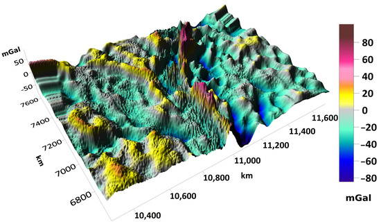
Figure 1.
Graph of the “residual” field (the difference between the observed field and the field of the initial approximation model).
Table 2.
Characteristics of the observed field, the initial approximation model field, and their difference—the “residual” field.
Let us describe the method for choosing the parameter to solve the inverse problem. Note that during minimizing the functional , the requirements for minimizing the error in the field while simultaneously minimizing the functional in a certain sense contradict each other. That is, as increases, there are small deviations in from zero, but a large discrepancy in the field. Thus, when solving a linear inverse problem of gravimetry with a restriction on the permissible values of the density of gravitating elements, there will always be a certain minimum achievable limit of field discrepancy, which may not always satisfy the desired accuracy.
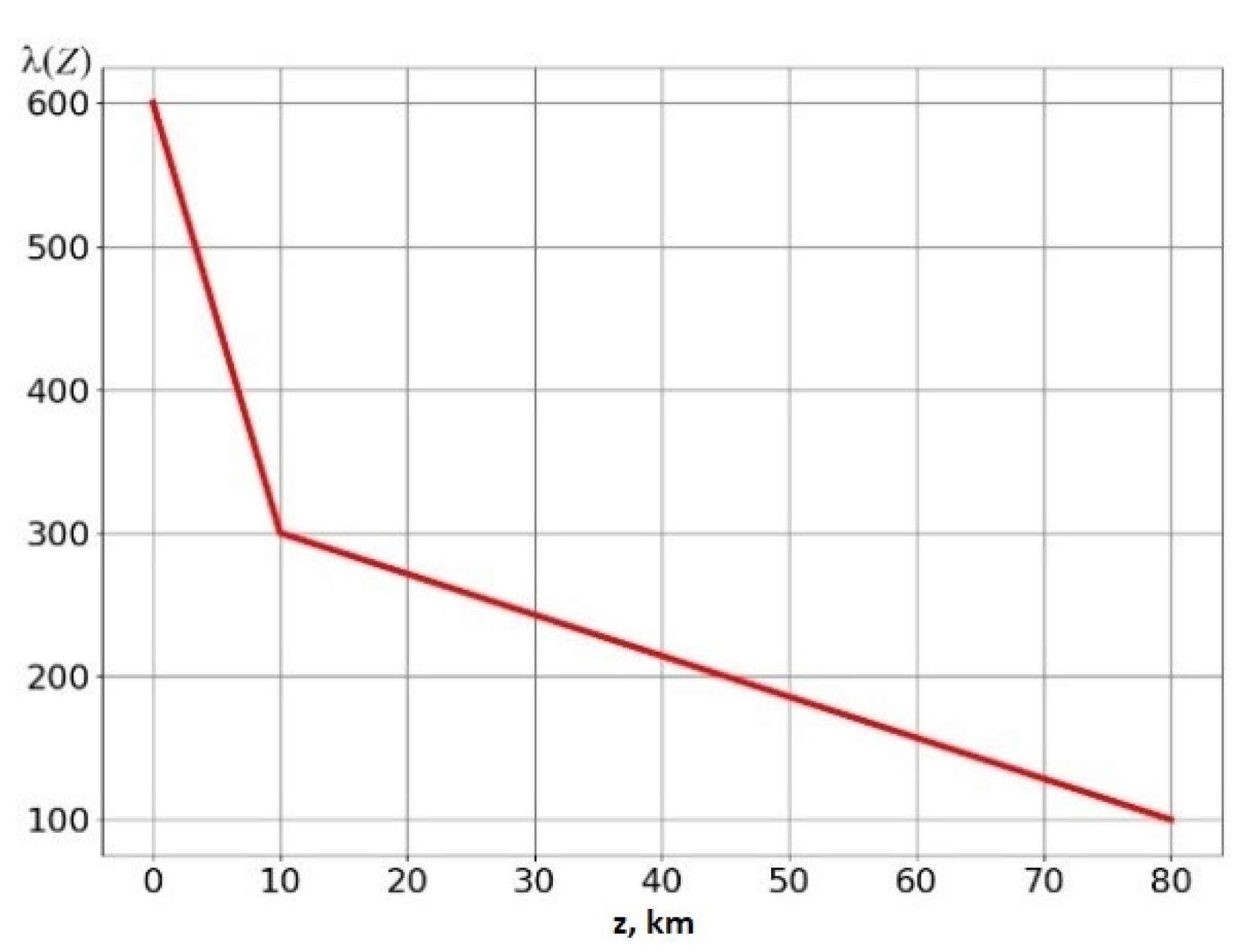
We conducted experiments with the choice of parameter to solve our practical problem. Table 3 shows some parameters of the resulting solution depending on the choice of . Figure 2 plots the resulting correction for the density distribution of the initial approximation model as a function of . At small values of the parameter , all high-amplitude values in are concentrated in the upper (closest to the field setting points) layer. As increases, the “high-frequency” components of the density distribution function remain in the upper layers, and the “low-frequency” ones fall into the lower layers. However, with a constant value of , when the desired values of the deviation from zero (±0.2 g/cm3) are achieved, the field discrepancy turns out to be unsatisfactory. Therefore, we moved to a more “flexible” assignment of . In Formula (14), we replaced the diagonal matrix with identical elements on the main diagonal with a diagonal matrix with different elements , depending on the depth of the corresponding element of the model partition. The function (see Figure 3) was chosen experimentally with the condition of imposing a larger “penalty” for large amplitudes in the upper layers. With this choice of , we obtained a relative field error of 3.3% with satisfactory deviations of the final density distribution from the initial approximation model.
Table 3.
Influence of the parameter on the resulting solution.
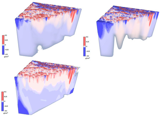
Figure 2.
Correction of the initial approximation model’s density distribution at (top left), (top right), and (bottom left).
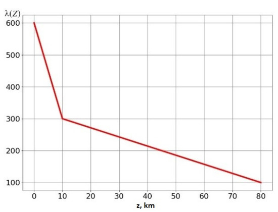
Figure 3.
The function chosen for the final solution.
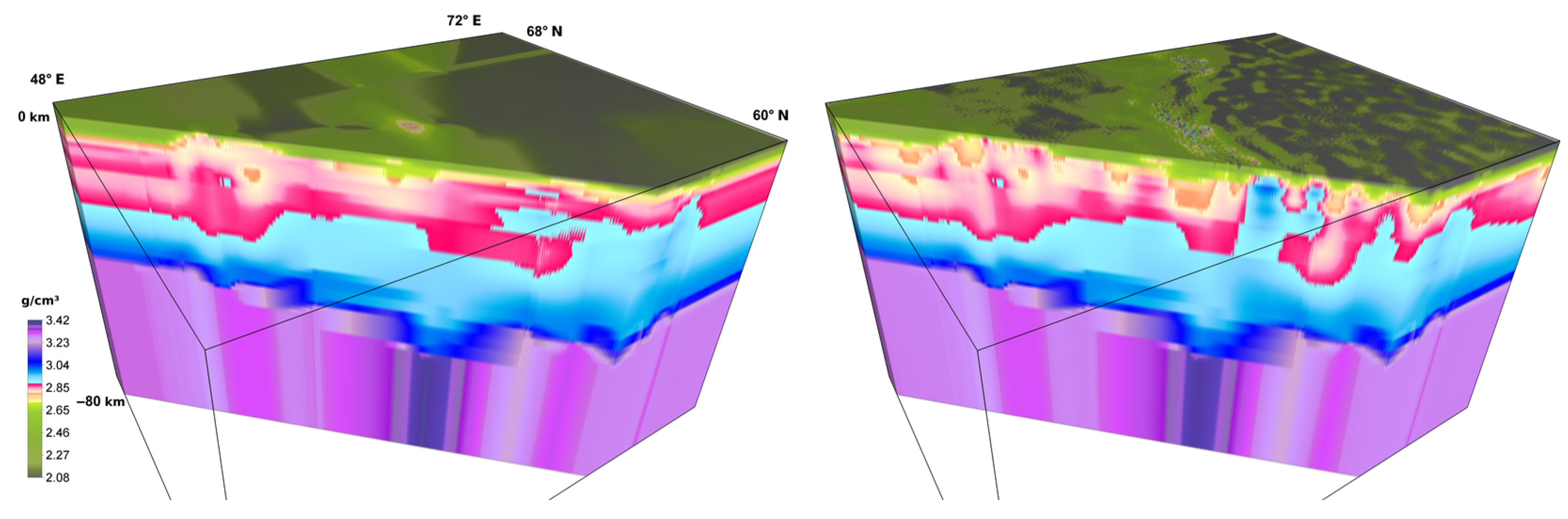
It took 39 iterations of the parallel method (approx. 2.5 h using 3 AMD Radeon™ VII and 2 AMD Radeon™ RX5700XT GPUs) to construct a solution until the residual in the field reached 3% (and error in the minimized functional reached 0.3%). Figure 4 shows the density model of the initial approximation and the result of solving the inverse problem (the relief is practically invisible on the scale of the figure). The densities of the relief-forming rock layer are shown in Figure 5. Table 4 shows the characteristics of the models.
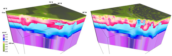
Figure 4.
Density model of the initial approximation (left) and the resulting model (right). A diagonal cut has been made.
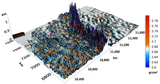
Figure 5.
The result of solving the inverse problem: the density in a layer of relief-forming rocks.
Table 4.
Characteristics of density models.
Despite the almost 100% difference between the observed field and the field of the initial approximation model, very small (in terms of relative deviation) corrections to the model were required to reduce the discrepancy. These corrections are localized mainly in the upper layers of the model, where their influence is especially noticeable.
5. Conclusions
An original algorithm for solving a three-dimensional inverse linear gravimetry problem has been developed and implemented in software (based on the performance algorithm for solving the forward problem). The solution is achieved by using the conjugate gradient method with the introduction of additional optimization conditions. A method is proposed for introducing a target functional, the minimization of which (with restrictions imposed on the desired solution) allows one to narrow down the set of feasible solutions. The introduced restrictions correspond to a priori information about the density distribution, and also have a small number of “free” or “tuning” parameters. The implemented algorithm is optimal: the main calculation time is comprised of multiple runs of the forward problem program. Thanks to this structure of the algorithm, further optimizations can be carried out only for the program for solving the forward problem. The conducted tests show that it is now possible to interpret observed gravity data without first calculating corrections for the topography, using anomalies in free air to create the spherical density models. This paper provides an example of such an interpretation based on parallel algorithms developed by the authors and implemented using distributed computing on graphic accelerators of personal computers. A solution to a practical three-dimensional inverse problem of gravimetry for the Urals region has been obtained, taking the topography into account; a digital density model of the Earth’s crust has been created using the observed gravity data. The effectiveness of the interpretation method developed by the authors does not depend on the regularity of either the density model grids or the calculated field. In this case, the parameters of the density model, limited by surface topography, are determined. This approach will significantly improve the accuracy of determining model parameters.
Author Contributions
Conceptualization, P.M. and D.B.; methodology, P.M. and D.B.; software, D.B.; validation, P.M. and D.B.; formal analysis, P.M.; investigation, P.M. and D.B.; writing—original draft preparation, P.M. and D.B.; writing—review and editing, P.M. and D.B.; visualization, D.B.; supervision, P.M.; project administration, P.M.; funding acquisition, P.M. All authors have read and agreed to the published version of the manuscript.
Funding
This research received no external funding.
Data Availability Statement
The data will be made available by the authors on request.
Conflicts of Interest
The authors declare no conflicts of interest. The funders had no role in the design of the study; in the collection, analyses, or interpretation of data; in the writing of the manuscript; or in the decision to publish the results.
References
- Lowrie, W.; Fichtner, A. Fundamentals of Geophysics, 3rd ed.; Cambridge University Press: Cambridge, UK, 2020; 426p. [Google Scholar] [CrossRef]
- Martyshko, P.S.; Byzov, D.D.; Chernoskutov, A.I. Interpretation of gravity data measured by topography. Dokl. Earth Sci. 2020, 495, 914–917. [Google Scholar] [CrossRef]
- Heck, B.; Seitz, K. A comparison of the tesseroid, prism and point-mass approaches for mass reductions in gravity field modelling. J. Geod. 2007, 81, 121–136. [Google Scholar] [CrossRef]
- Wild-Pfeiffer, F.; Augustin, W.; und Heck, B. Optimierung der Rechenzeit bei der Berechnung der 2. Ableitungen des Gravitationspotentials von Massenelementen. Z. Für Geodäsie 2007, 6, 377–384. [Google Scholar]
- Uieda, L.; Barbosa, V.; Braitenberg, C. Tesseroids: Forward-modeling gravitational fields in spherical coordinates. Geophysics 2016, 81, F41–F48. [Google Scholar] [CrossRef]
- Bouman, J.; Ebbing, J.; Meekes, S.; Fattah, R.A.; Fuchs, M.; Gradmann, S.; Haagmans, R.; Lieb, V.; Schmidt, M.; Dettmering, D.; et al. GOCE gravity gradient data for lithospheric modeling. Int. J. Appl. Earth Obs. Geoinf. 2015, 35A, 16–30. [Google Scholar] [CrossRef]
- Pedersen, L.B.; Kamm, J.; Bastani, M. A priori models and inversion of gravity gradient data in hilly terrain. Geophys. Prospect. 2020, 68, 1072–1085. [Google Scholar] [CrossRef]
- Laramie, V.P.; Ralph, R.B. Comprehensive mass modeling of the Moon from spectrally correlated free-air and terrain gravity data. J. Geophys. Res. 2003, 108, 5024. [Google Scholar] [CrossRef]
- EPSG Geodetic Parameter Dataset. Available online: https://epsg.org/ellipsoid_7030/WGS-84.html (accessed on 3 March 2024).
- Martyshko, P.S.; Ladovsky, I.V.; Byzov, D.D.; Chernoskutov, A.I. On solving the forward problem of gravimetry in curvilinear and Cartesian coordinates: Krasovskii’s ellipsoid and plane modeling. Izv. Phys. Solid Earth 2018, 54, 565–573. [Google Scholar] [CrossRef]
- Prudnikov, A.P.; Brychkov, Y.A.; Marichev, O.I. Integrals and series. In Elementary Functions, 2nd ed.; FIZMATLIT: Moscow, Russia, 2002; 632p, ISBN 5-9221-0323-7. [Google Scholar]
- Van Oosterom, A.; Strackee, J. The Solid Angle of a Plane Triangle. IEEE Trans. Biomed. Eng. 1983, 30, 125–126. [Google Scholar] [CrossRef] [PubMed]
- Henk, A.; van der Vorst, H.A. Iterative Krylov Methods for Large Linear System; Cambridge University Press: Cambridge, UK, 2003; 221p. [Google Scholar] [CrossRef]
- Ince, E.S.; Barthelmes, F.; Reißland, S.; Elger, K.; Förste, C.; Flechtner, F.; Schuh, H. ICGEM—15 years of successful collection and distribution of global gravitational models, associated services and future plans. Earth Syst. Sci. Data 2019, 11, 647–674. [Google Scholar] [CrossRef]


Disclaimer/Publisher’s Note: The statements, opinions and data contained in all publications are solely those of the individual author(s) and contributor(s) and not of MDPI and/or the editor(s). MDPI and/or the editor(s) disclaim responsibility for any injury to people or property resulting from any ideas, methods, instructions or products referred to in the content. |
© 2024 by the authors. Licensee MDPI, Basel, Switzerland. This article is an open access article distributed under the terms and conditions of the Creative Commons Attribution (CC BY) license (https://creativecommons.org/licenses/by/4.0/).