
Simple Moment Generating Function Optimisation Technique to Design Optimum Electronic Filter for Underwater Wireless Optical Communication Receiver
 , , and
Abstract
:1. Introduction
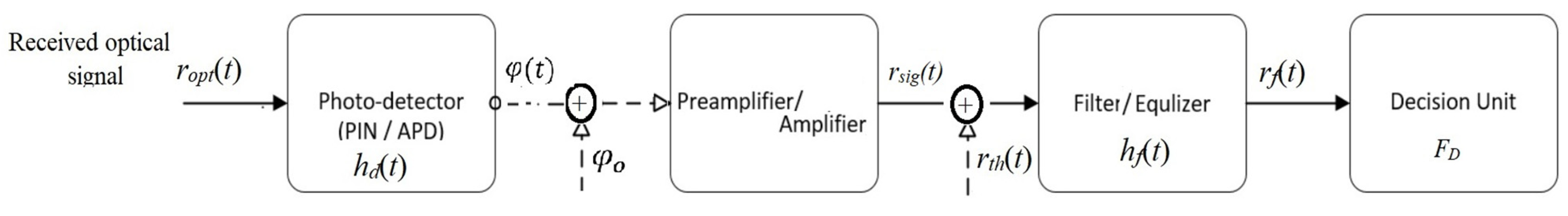
2. Optical Receiver Mathematical Design Model
3. Optical Receiver Filter Equation–MGF Optimisation Procedure
3.1. MGF and LMGF for Optical Receiver Signal
3.2. MGF-Based Model for Time-Invariant Rx System
3.2.1. Use Case I: rsig(t) without AGTN Noise and ISI
3.2.2. Use Case II: rsig(t) with White AGTN Noise and ISI
3.2.3. Use Case III: rsig(t) with Colored AGTN Noise and ISI
3.3. Optimum Filter Impulse Response Function
4. Results and Discussion
4.1. MGF Model Validation
4.2. Software Implementation Notes
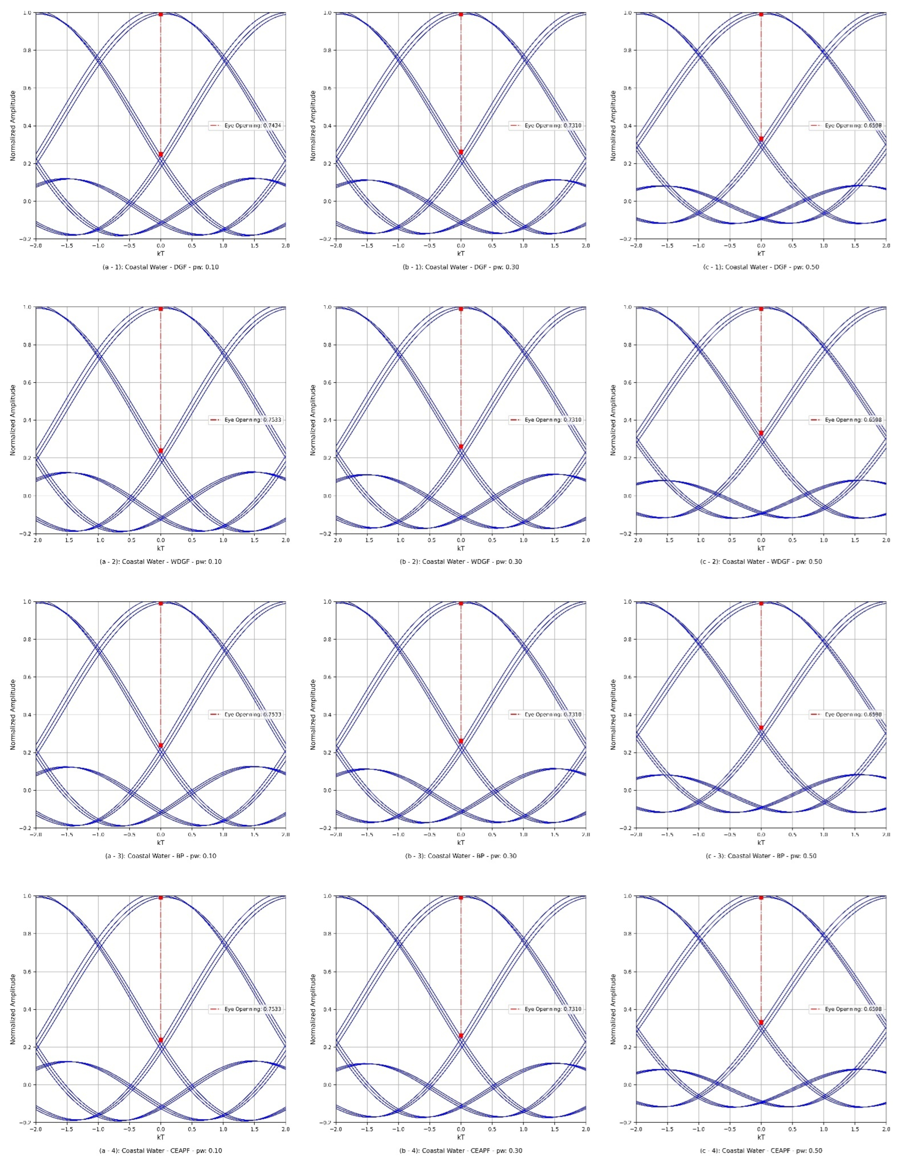
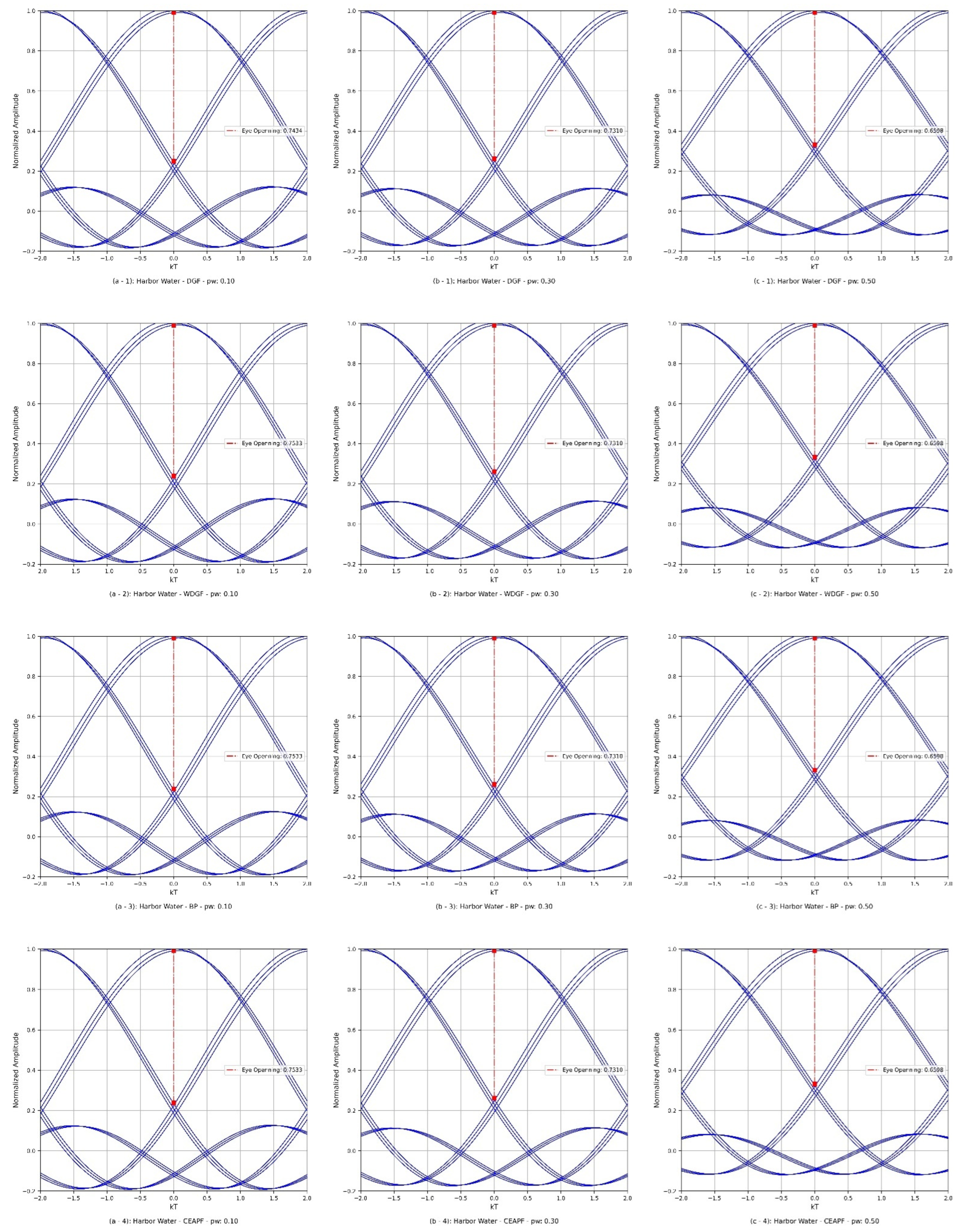
4.3. Computation Data Visualisation
5. Conclusions and Future Work
Author Contributions
Funding
Data Availability Statement
Acknowledgments
Conflicts of Interest
References
- Tang, S.; Dong, Y.; Zhang, X. Impulse response modeling for underwater wireless optical communication links. IEEE Trans. Commun. 2013, 62, 226–234. [Google Scholar] [CrossRef]
- Dong, Y.; Zhang, H.; Zhang, X. On impulse response modeling for underwater wireless optical MIMO links. In Book on Impulse Response Modeling for Underwater Wireless Optical MIMO Links; IEEE: Shanghai, China, 2014; pp. 151–155. [Google Scholar]
- Li, Y.; Leeson, M.S.; Li, X. Impulse response modeling for underwater optical wireless channels. Appl. Opt. 2018, 57, 4815–4823. [Google Scholar] [CrossRef] [PubMed]
- Cox, W.C., Jr. Simulation, Modeling, and Design of Underwater Optical Communication Systems. Ph.D. Thesis, North Carolina State University, Raleigh, NC, USA, 2012. [Google Scholar]
- Zhang, H.; Dong, Y. General stochastic channel model and performance evaluation for underwater wireless optical links. IEEE Trans. Wirel. Commun. 2015, 15, 1162–1173. [Google Scholar] [CrossRef]
- Boluda-Ruiz, R.; Rico-Pinazo, P.; Castillo-Vázquez, B.; García-Zambrana, A.; Qaraqe, K. Impulse response modeling of underwater optical scattering channels for wireless communication. IEEE Photonics J. 2020, 12, 1–14. [Google Scholar] [CrossRef]
- Elamassie, M.; Miramirkhani, F.; Uysal, M. Performance characterization of underwater visible light communication. IEEE Trans. Commun. 2018, 67, 543–552. [Google Scholar] [CrossRef]
- Al-Zhrani, S.; Bedaiwi, N.M.; El-Ramli, I.F.; Barasheed, A.Z.; Abduldaiem, A.; Al-Hadeethi, Y.; Umar, A. Underwater optical communications: A brief overview and recent developments. Eng. Sci. 2021, 16, 146–186. [Google Scholar] [CrossRef]
- Personick, S.D. Receiver design for digital fiber optic communication systems, I. Bell Syst. Tech. J. 1973, 52, 843–874. [Google Scholar] [CrossRef]
- House, K. Detection and Equalization in Fiber-Optic Communication. Ph.D. Thesis, University of Essex, Colchester, UK, 1979. [Google Scholar]
- House, K. Filters for the detection of binary signaling: Optimization using the Chernoff bound. IEEE Trans. Commun. 1980, 28, 257–259. [Google Scholar] [CrossRef]
- Da Rocha, J.; Oreilly, J. Modified Chernoff bound for binary optical communication. Electron. Lett. 1982, 18, 708–710. [Google Scholar] [CrossRef]
- Da Rocha, J.; O’Reilly, J. Linear direct-detection fiber-optic receiver optimization in the presence of intersymbol interference. IEEE Trans. Commun. 1986, 34, 365–374. [Google Scholar] [CrossRef]
- O’Reilly, J.; Watkins, L.; Schumacher, K. New strategy for the design and realisation of optimised receiver filters for optical telecommunications. IEE Proc. J. Optoelectron. 1990, 137, 181–185. [Google Scholar] [CrossRef]
- Al-Ramli, I.F.K. Receiver Structures and Filter Characteristics for M-Ary Optical Communication Systems. Ph.D. Thesis, University of Essex, Colchester, UK, 1985. [Google Scholar]
- Al-Ramli, F. Optimum Receiver Structure and Filter Design for MPAM Optical Space Communication Systems. In Laser in der Technik/Laser in Engineering; Springer: Munich, Germany, 1992; pp. 192–195. [Google Scholar]
- El-Hadidi, M.; Hirosaki, B. The Bayes’ optimal receiver for digital fibre optic communication systems. Opt. Quantum Electron. 1981, 13, 469–486. [Google Scholar] [CrossRef]
- Foulds, L.R. Optimization Techniques: An Introduction; Springer Science & Business Media: Berlin/Heidelberg, Germany, 2012. [Google Scholar]
- Chen, Y.; Kong, M.; Ali, T.; Wang, J.; Sarwar, R.; Han, J.; Guo, C.; Sun, B.; Deng, N.; Xu, J. 26 m/5.5 Gbps air-water optical wireless communication based on an OFDM-modulated 520-nm laser diode. Opt. Express 2017, 25, 14760–14765. [Google Scholar] [CrossRef] [PubMed]
- Wu, T.C.; Chi, Y.C.; Wang, H.Y.; Tsai, C.T.; Lin, G.R. Blue laser diode enables underwater communication at 12.4 Gbps. Sci. Rep. 2017, 7, 40480. [Google Scholar] [CrossRef] [PubMed]
- Ramavath, N.; Udupi, S.A.; Krishnan, P. High-speed and reliable Underwater Wireless Optical Communication system using Multiple-Input Multiple-Output and channel coding techniques for IoUT applications. Opt. Commun. 2020, 461, 125229. [Google Scholar] [CrossRef]
- Li, C.; Lu, H.; Wang, W.; Hung, C.; Su, C.; Lu, Y. A 5 m/25 Gbps underwater wireless optical communication system. IEEE Photonics J. 2018, 10, 7904909. [Google Scholar] [CrossRef]
- Wang, K.; Gao, Y.; Dragone, M.; Petillot, Y.; Wang, X. Advanced Underwater Wireless Optical Communication System Assisted by Deep Echo State Network. In Proceedings of the 2022 Asia Communications and Photonics Conference (ACP), Shenzhen, China, 5–8 November 2022. [Google Scholar] [CrossRef]
- Kong, M.; Guo, Y.; Sait, M.; Alkhazragi, O.; Kang, C.H.; Ng, T.K.; Ooi, B.S. Underwater optical wireless sensor network for real-time underwater environmental monitoring. Next-Gener. Opt. Commun. 2022, 12028, 82–86. [Google Scholar] [CrossRef]
- Tao, H.; Zhiqiang, F.; Jun, S.; Qi, Q. Real-Time Eye Diagram Monitoring for Optical Signals Based on Optical Sampling. Appl. Sci. 2023, 13, 1363. [Google Scholar] [CrossRef]
- Cattermole, K.W.; O’Reilly, J.J. Mathematical Topics in Telecommunications, Optimisation in Electronics and Communications; Wiley: New York, NY, USA, 1984. [Google Scholar]
- Gagliardi, R.M.; Karp, S. Optical Communications; Wiley: New York, NY, USA, 1976. [Google Scholar]
- Saleh, B. Photoelectron Statistics: With Applications to Spectroscopy and Optical Communication; Springer: Berlin/Heidelberg, Germany, 2013. [Google Scholar]
- Govind, P. Agrawal: “Fiber-Optic Communication Systems”, 4th ed.; A John Wiley & Sons, Inc.: Hoboken, NJ, USA, 2010. [Google Scholar]
- Sanjeev, K.R.; Nimish, K.S.; Akash, S. A novel approach to generate a chirp microwave waveform using temporal pulse shaping technique applicable in remote sensing application. Int. J. Electron. 2017, 104, 1689–1699. [Google Scholar] [CrossRef]
- Wolfgang, F.; René, S.; Bernd, N.; Marcus, W.; Arne, J.; David, H.; Swen, K.; Joachim, M.; Michael, D.; Michael, H.; et al. Quality Metrics for Optical Signals: Eye Diagram, Q-factor, OSNR, EVM and BER. In Proceedings of the 2012 14th International Conference on Transparent Optical Networks (ICTON), Coventry, UK, 2–5 July 2012. [Google Scholar]
- Ippei, S.; Hidehiko, T.; Satoki, K. Simple Measurement of Eye Diagram and BER Using High-Speed Asynchronous Sampling. J. Light. Technol. 2004, 22, 5. [Google Scholar] [CrossRef]


| Use Case | Water Type | Equation | ISI | Computation Attributes {N0, a0, a1, pw} | |||
|---|---|---|---|---|---|---|---|
| General | Optimum | Filter | Without (Signal Only = Path Loss Channel) | With | |||
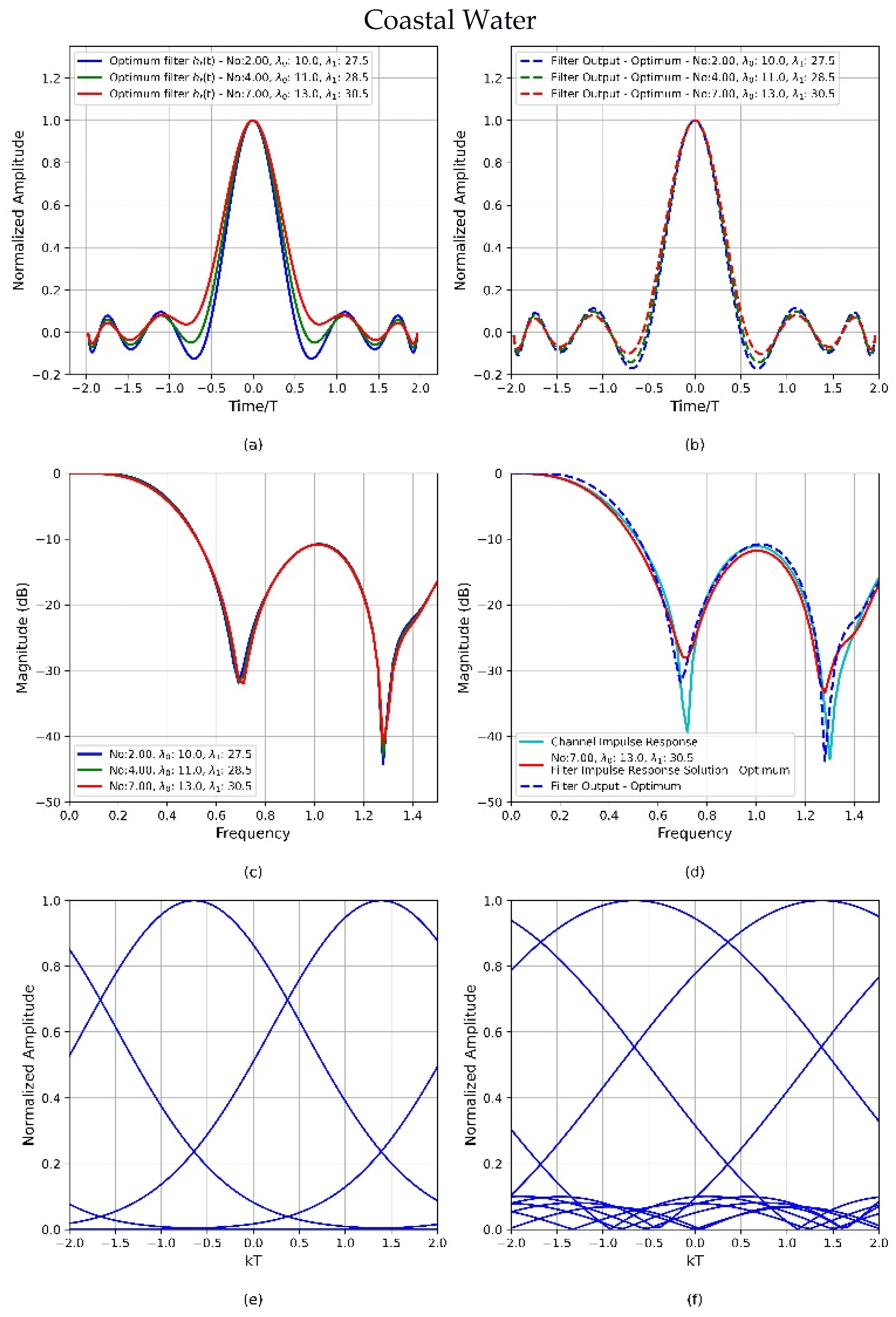
| III (Figure 4) | Coastal | (15) | (20) | (15) | {a, b, c} | {d, e, f} | {0.0, 3.0, 13., 0.25} |
| III (Figure 5) | Coastal | (17) | (21) | (18, 23) | {a, b, c} | {d, e, f} | {2.75,10, 20, 0.25} |
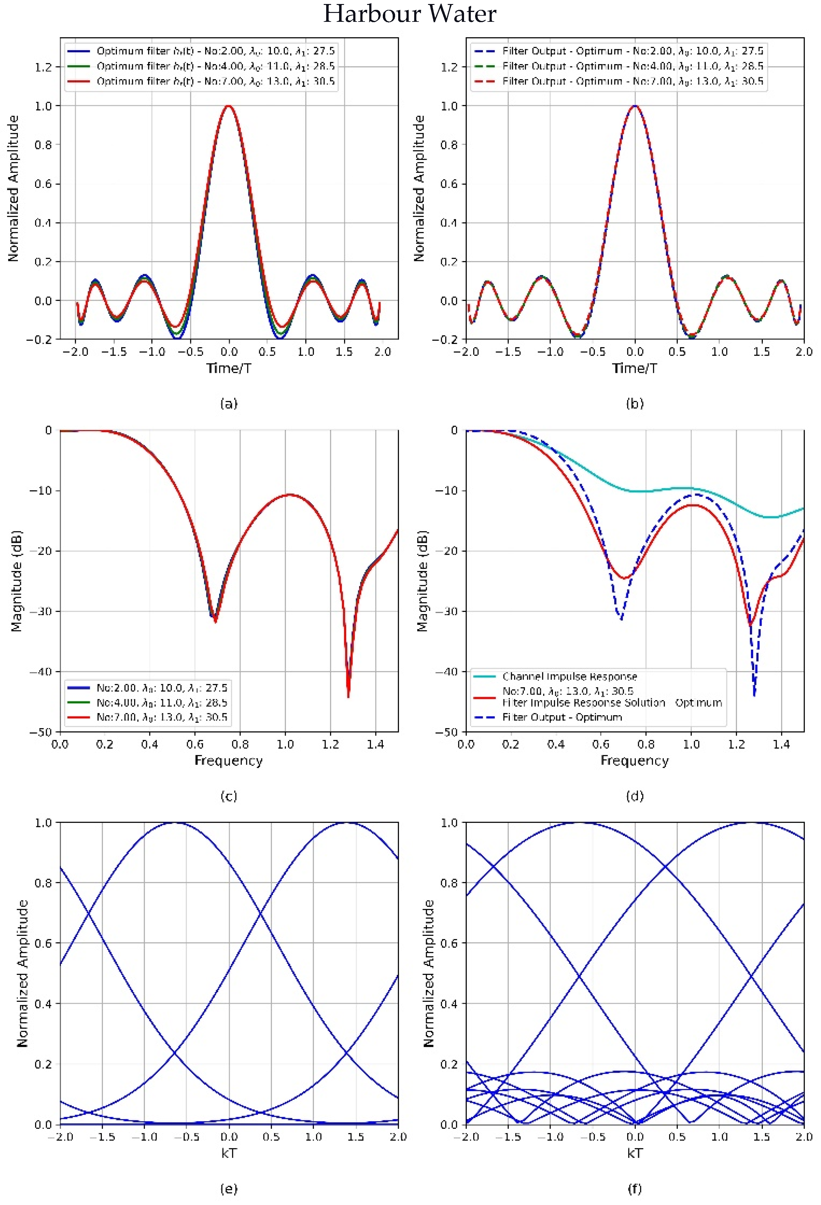
| III (Figure 6) | Coastal, Harbour | (19) | (22) | {a, b, c, d, e, f} | Several sets in Figure 6 | ||
Disclaimer/Publisher’s Note: The statements, opinions and data contained in all publications are solely those of the individual author(s) and contributor(s) and not of MDPI and/or the editor(s). MDPI and/or the editor(s) disclaim responsibility for any injury to people or property resulting from any ideas, methods, instructions or products referred to in the content. |
© 2024 by the authors. Licensee MDPI, Basel, Switzerland. This article is an open access article distributed under the terms and conditions of the Creative Commons Attribution (CC BY) license (https://creativecommons.org/licenses/by/4.0/).
Share and Cite
Ramley, I.F.E.; AlZhrani, S.M.; Bedaiwi, N.M.; Al-Hadeethi, Y.; Barasheed, A.Z. Simple Moment Generating Function Optimisation Technique to Design Optimum Electronic Filter for Underwater Wireless Optical Communication Receiver. Mathematics 2024, 12, 861. https://doi.org/10.3390/math12060861
Ramley IFE, AlZhrani SM, Bedaiwi NM, Al-Hadeethi Y, Barasheed AZ. Simple Moment Generating Function Optimisation Technique to Design Optimum Electronic Filter for Underwater Wireless Optical Communication Receiver. Mathematics. 2024; 12(6):861. https://doi.org/10.3390/math12060861
Chicago/Turabian StyleRamley, Intesar F. El, Saleha M. AlZhrani, Nada M. Bedaiwi, Yas Al-Hadeethi, and Abeer Z. Barasheed. 2024. "Simple Moment Generating Function Optimisation Technique to Design Optimum Electronic Filter for Underwater Wireless Optical Communication Receiver" Mathematics 12, no. 6: 861. https://doi.org/10.3390/math12060861