Profiling Social Sentiment in Times of Health Emergencies with Information from Social Networks and Official Statistics

Abstract

Social networks and official statistics have become vital sources of information in times of health emergencies. The ability to monitor and profile social sentiment is essential for understanding public perception and response in the context of public health crises, such as the one resulting from the COVID-19 pandemic. This study will explore how social sentiment monitoring and profiling can be conducted using information from social networks and official statistics, and how this combination of data can offer a more complete picture of social dynamics in times of emergency, providing a valuable tool for understanding public perception and guiding a public health response. To this end, a three-layer architecture based on Big Data and Artificial Intelligence is presented: the first layer focuses mainly on collecting, storing, and governing the necessary data such as social media and official statistics; in the second layer, the representation models and machine learning necessary for knowledge generation are built, and in the third layer the previously generated knowledge is adapted for better understanding by crisis managers through visualization techniques among others. Based on this architecture, a KDD (Knowledge Discovery in Databases) framework is implemented using methodological tools such as sentiment analysis, fuzzy 2-tuple linguistic models and time series prediction with the Prophet model. As a practical demonstration of the proposed model, we use tweets as data source (from the social network X, formerly known as Twitter) generated during the COVID-19 pandemic lockdown period in Spain, which are processed to identify the overall sentiment using sentiment analysis techniques and fuzzy linguistic variables, and combined with official statistical indicators for prediction, visualizing the results through dashboards.

1. Introduction

In the last few years, the world has faced multiple health-related crises, including the Ebola outbreak in 2014, Zika in 2015, Dengue in 2019, and most recently, the COVID-19 pandemic in 2020. These crises have had a profound impact on public health and the global economy. In addition, financial crises and geopolitical pressures have increased uncertainty in both markets and political stability. Moreover, these crises have left a significant social impact on various social groups worldwide. The COVID-19 pandemic, in particular, has highlighted existing inequalities, disproportionately affecting vulnerable groups and widening such socio-economic disparities.

These challenges have emphasized the importance of having a well-prepared and systematic approach to health crisis management. On the one hand, there is evidence of the relevance of expert information that can be provided by official statistical sources [1]. Among other indicators, monitoring of “social sentiment”, which has been captured in surveys conducted by official bodies such as the Centro de Investigaciones Sociológicas (CIS (https://www.cis.es/detalle-ficha-estudio?origen=estudio&idEstudio=14551) accessed on 1 January 2024) in Spain, has become relevant. On the other hand, through the use of social networks, citizens have a mechanism for conveying their feelings. Social networks have revolutionized the way people communicate and share information and have thereby become a crucial forum for expressing and monitoring public reactions to health crises. Their influence on the perception of and response to these crises is significant [2]. The usefulness of such information for crisis management is therefore beyond doubt. This information source is processed by natural language processing (NLP) techniques and can be used for the same purpose of gathering feelings through surveys such as the one by CSIC mentioned above. This can reveal how the population feels about the emergency at hand and, consequently, help identify emerging trends such as symptoms, treatments, or logistical challenges. These trends can inform authorities on areas where they should focus their efforts to manage public concerns.

While social networks serve as a mechanism for understanding the collective mindset, official statistics offer a solid foundation for validating and contextualizing information. Data provides crucial context for comprehending the severity of emergencies and their impact on society, aiding in the assessment of the effectiveness of public health measures and their acceptance by the population. Integrating data from official statistics and social networks into sentiment profiling can be a powerful tool for health emergency management. Indeed, by understanding how the population perceives and reacts to the crisis, health authorities can (1) adjust communication strategies to address specific concerns; assess the effectiveness of public health measures; (2) identify emerging challenges, such as atypical symptoms or lack of medical supplies; and (3) make informed and adaptive decisions in real time. It is therefore essential for agile, evidence-based decision making in times of health emergencies, and this methodology has significant potential to improve the response to future public health emergencies. Effective crisis management must then use a variety of sources, which are often generated in real-time and may also be unstructured. Therefore, a Big Data and Artificial Intelligence-based architecture may be appropriate to manage all this information for effective crisis management.

This research endeavors to investigate the implementation of social sentiment monitoring through the combination of data sources from social networks (for the endogenous variable sentiment analysis) and official statistics, particularly focusing on series that significantly impact the endogenous variable. The objective is to elucidate how integrating these diverse data sources can provide a more comprehensive understanding of social dynamics during emergencies, thereby supplementing the insights derived from official statistical indicators [3,4]. For this purpose, we present an architecture founded on Big Data and Artificial Intelligence, as outlined in [5], designed to tackle a case study on crisis management, specifically centered on the first lockdown in Spain during the COVID-19 crisis. Following this, we offer a more in-depth explanation of these layers (refer to Figure 1):

• Data Management Solutions for Social Analytics (DMSSA): This layer plays a crucial role in allowing organizations to collect, store, organize, tag, and govern the data needed for crises: social media, financial and economic data, health data, political and social data, etc. These data are usually not free of uncertainty, especially those coming from social networks. Since the objective is to monitor social sentiment, social network data are the primary data source, complemented by other reliable data sources such as data from official health statistics, public health records, economic indicators, etc. that can be accessed relatively quickly to feed the model.
• Insight Generation for Society (IGS): In this layer, we build the representation models, sentiment analysis, and machine learning necessary for the generation of knowledge that allows the anticipation of social problems arising from the crisis. Undoubtedly, there is uncertainty in the information expressed in the natural language of social networks; therefore, this paper will propose the use of fuzzy 2-tuple linguistic modeling as a representation of such information, which has been successfully used in similar circumstances [6,7,8,9], allowing the complexities presented in the linguistic expressions related to feelings to be captured. Finally, for better crisis management, time series prediction techniques are applied to allow the system manager to foresee events and the inclusion of external regressors from official data sources is expected to improve the predictive capabilities of the models.
• Social Application (SA): the previously generated knowledge is adapted for better understanding by crisis managers through visualization techniques, monitoring, warning generation, etc. These tools can be integrated into dashboards to facilitate informed decision making.

The rest of the study is structured as follows: Section 2 discusses the related work, highlighting the originality of our proposal. Section 3 explains the main pillars of the proposed model. In Section 4, we address a case of social monitoring during the COVID-19 pandemic in Spain, within the framework of the aforementioned architecture, following the typical phases of a data science project. The obtained results are deliberated in Section 5, while conclusions and future prospects are outlined in Section 6.

2. Related Works

This Section reviews the existing research works involved in the monitoring of social media data and how each of them relates to the architecture proposed here.

Simranpreet et al. [10] describe the monitoring of the dynamics of emotions during COVID-19 using X (formerly known as Twitter) data and TextBlob for analyzing sentiment. Moreover, IBM Cloud is employed to predict the emotional tone associated with the text, aiming to extract information about the user’s emotional engagement while writing the tweet. Kambiz et al. [11] focus on monitoring and recommending systems for privacy settings for the social network Facebook using KNN in Weka to classify the participants based on their disclosed common personal information. Alexander et al. [12] assess the impacts of participation and network ties on the decisions of fishers to voluntarily report rule violations in two Jamaican marine reserves using a logistic regression model for analysis. Thin et al. [13] investigate whether the content contributed by members of the depression community to community blogs differs from what they post on their personal blogs, employing Lasso as the classifier, Feature Selector, and Statistical Testing for analysis. In their study, Nepali et al. [14] introduce a social network model called SONET, designed for privacy monitoring and ranking. This model offers a fresh, efficient, and pragmatic approach to quantifying, assessing, and evaluating privacy concerns. Piedrahita-Valdés et al. [15] examine the role of vaccine-related discussions on social media in identifying factors influencing vaccine confidence across various historical periods and geographical regions. Zucco et al. [16] examine techniques and resources for analyzing textual and social network data sources to extract sentiment. Meanwhile, Sufi et al. [17] conduct an analysis of locally focused public sentiments regarding global disaster events. Their study is the first to integrate location intelligence with sentiment analysis, regression, and anomaly detection applied to social media messages concerning disasters, covering a wide array of languages. Tran et al. [18] track the well-being of vulnerable transit riders during the COVID-19 period by employing machine learning-based sentiment analysis and social media data. Finally, El Barachi et al. [19] develop a framework capable of providing real-time insights into the evolution of public opinion.

A summary of the data, the analysis technique, and the sentiment representation techniques used are provided in

Table 1. Related works.

Ref.	DMSSA	IGS	SA
Kaur et al. [10]	A total of 16,138 COVID-19 related tweets from February to June 2020.	TextBlob for sentiment (−1, 1)	Static tables and graphs
Ghazinour et al. [11]	Data collected from three Facebook users	KNN in Weka with K = 3 to classify the participants	Static tables and graphs
Alexander at al. [12]	Questionnaires with fishers (n = 277)	logistic regression model	Static tables and graphs
Nguyen et al. [13]	A total of 25,012 community posts and 104,033 personal posts crawled from depression.livejournal.com	Lasso as the Classifier and Feature Selector, Statistical Testing	Static tables and graphs
Nepali et al. [14]	Search results from an existing search engine, such as Google and Bing, and deep web searches	PIDX algorithm	None
Piedrahita-Valdés et al. [15]	Vaccine-related tweets published on Twitter from 1 June 2011 to 30 April 2019.	SVM classifier, One-way ANOVA, Kruskal–Wallis… Positive, negative, and neutral polarity	Static tables and graphs
Zucco, Chiara et al. [16]	Polarity detection	Detection of subjectivity; SFE, extraction of semantic features; SL, sentence level; WL, word level	Static tables and graphs
Sufi et al. [17]	Twitter feeds from 28 September to 6 October 2021	Named entity recognition (NER), anomaly detection, regression, and the Getis Ord Gi* algorithms	Static tables and graphs
Tran et al. [18]	The Twitter dataset captures the travel experiences of approximately 120,000 transit riders in Metro Vancouver, Canada, both before and during the pandemic.	Sentiment analysis	Static tables and graphs
El Barachi, May et al. [19]	A total of 278,000 tweets related to the topic of climate change	LSTM classifier	Static tables and graphs
Our proposal	∼4.5 million tweets	Sentiment analysis, 2-tuples, and time series analysis	Interactive dashboard

. None of these works provide an interactive dashboard for effective crisis management that can be analyzed almost in real-time. Also, none of these frameworks use a 2-tuples fuzzy linguistic approach, which allows a continuous representation of the linguistic information in its domain.

3. Methods and Materials

For the development of the proposed system, sentiment detection techniques have been used, the polarity of the detected sentiments has been represented by the fuzzy 2-tuple linguistic model, and also time series has been used for the prediction of the sentiment. The fundamentals are explained below.

3.1. Sentiment Analysis

To determine the sentiment expressed in an opinion, different techniques can be used [20]. Particularly, in our case study, traditional machine learning has been used, as well as semantic-based, and pre-trained language models tech.

On the one hand, with traditional machine learning techniques, patterns can be found among the published messages that determine whether they are positive or negative. Particularly, the labeled dataset is partitioned into a training set (70%) and a test set (30%), and the models neural network, naïve Bayes, SVM, XGBoost [21], and K-Nearest Neighbor [22] are used for sentiment detection.

On the other hand, a masked language model based on transformers’ semantic-based techniques are tested, using prefixed dictionaries where each word has a sentiment assigned to it. Within these techniques, two options are presented, the ISOL [23], where a set of words are used and assigned a value of 1 if they contribute positivity to a message, −1 otherwise, and 0 in case of neutrality. There are numerous examples of dictionaries in English, although not so many in Spanish. The one chosen for the project was the Spanish resource published in [24], composed of a total of 2509 positive words and 5626 negative words. Within this same paradigm of dictionaries is the Affective Norms for English Words (ANEW) lexicon model [25]. From this model, an adaptation to Spanish [26] known as Emotional norms for Spanish words (ENSW) is derived [27]. The sentiment values proposed in this paper combine and encapsulate both dimensions—quality and intensity of sentiment—into a singular score for each word, as detailed in [28]. Initially, arousals are linearly adjusted to a range between 0 and 1, representing minimum to maximum intensity. Subsequently, valences are mapped onto the interval [−4, 4] to reflect the negative/positive polarity by subtracting 5 from the original values. Assessing the sentiment strength for each word involves multiplying these adjusted valences by their corresponding precomputed weights (intensity). Thus, the weight alters the valence value in the appropriate direction, covering the entire intensity spectrum. To finalize these computations, the measures are translated to the interval [0, 1] to derive the ultimate sentiment value. The expression for the final computed score for each word ww is as follows:

$$s(w)=\left[\frac{\frac{arousal\left(w\right)-1}{8}·\left(valence\left(w\right)-5\right)}{8}\right]+4$$

(1)

The mean values of $arousal\left(w\right)$ and $valence\left(w\right)$ correspond to the word $w$ found in the ENSW dictionary. Consequently, words conveying positive sentiments are allocated higher values, while those with negative connotations are assigned lower values.

Lastly, the RoBERTa pre-trained language model is used [29]: The model known as roberta-base-bne is a masked language model based on transformers, specifically designed for the Spanish language. The model is built upon the RoBERTa base architecture and underwent pre-training utilizing the most extensive Spanish corpus available up to the present moment. This corpus comprises 570 GB of meticulously curated and deduplicated text specifically processed for this project. The content was sourced from web crawls conducted by the National Library of Spain (Biblioteca Nacional de España) spanning the years 2009 to 2019.

3.2. The 2-Tuple Fuzzy Linguistic Model

In the previous Section, we have seen several mechanisms for extracting the sentiment from natural language. Many authors have presented the advantage of interpretability of representing these feelings employing fuzzy linguistic variables (with labels such as Positive, Negative, and Neutral) instead of numbers [30]. A problem to be solved now is to compute (especially aggregate) these fuzzy labels without losing information. The 2-tuple model, as proposed by [31], aims to address the issue of information loss encountered in computational processes involving linguistic labels. This model has as its basis of representation a pair of values (${s_i,\alpha }_i)$, where $s$_i $\in$ S, represents the fuzzy linguistic label, and ${\alpha }_i\in [-0.5,0.5)$, signifies the symbolic translation from this label. The following provides a concise overview of the linguistic 2-tuple representation model and its computational framework.

Definition 1.

Let $S={\{s}_1,\dots ,s_g\}$ a set of linguistic terms and $\beta \in \left[1,g\right]$ a value in the granularity interval of S. The symbolic translation of a linguistic term, $s_i$, is a number valued in the interval $[-0.5,0.5)$ which expresses the difference in information between a quantity of information expressed by the value $\beta$obtained in a symbolic operation and the closest integer value $i,withi\in \{1,\dots ,g\}$, that indicates the index of the closest linguistic term in S.

This representation model establishes a pair of functions for converting numerical values within the granularity interval into 2-tuple linguistic values, facilitating computational processes involving 2-tuple linguistic values.

Definition 2.

Let a set of linguistic terms  $S=s_1,\dots ,s_g$, $\langle S\rangle =S\times [-0.5,0.5)$ and $\beta \in \left[1,g\right]$ a value representing the result of a symbolic operation, then the linguistic 2-tuple expressing information equivalent to $\beta$ is derived using the following function:

$$\begin{gathered} {∆}_S:\left[1,g\right]\to \langle S\rangle \\ {\mathsf{\Delta }}_S\left(\beta \right)=\left(s_i,{\alpha }_i\right),with\{i=round\left(\beta \right)and\alpha =\beta -i,\alpha \in [-0.5,0.5)\} \end{gathered}$$

(2)

Here, $\times$ denotes the Cartesian product between set $S$ and the real half-open interval [−0.5,0.5), while $round\left(·\right)$ represents the standard rounding operator. $s_i$ signifies the label closest to $\beta$ with an index, and $\alpha$ denotes the value of the symbolic translation. As a result, any value within the interval l $\left[1,g\right]$ is consistently associated with a 2-tuple linguistic value in $\langle S\rangle$.

Definition 3.

Let $S=s_1,\dots ,s_g$ a set of linguistic terms, and $\left(s_i,{\alpha }_i\right)\in \langle S\rangle =S\times [-\mathrm{0.5,0.5})$ the numerical value within the granularity interval $\left[1,g\right]$ representing the linguistic 2-tuple $\left(s_i,{\alpha }_i\right)$. This is obtained using the following function:

$$\begin{gathered} {\mathsf{\Delta }}_S^{-1}:\langle S\rangle \to \left[1,g\right] \\ {\mathsf{\Delta }}_S^{-1}\left(s_i,{\alpha }_i\right)=i+\alpha =\beta \end{gathered}$$

(3)

Definition 4.

Let $\left((s_1,{\alpha }_1\right),\dots ,(s_m,{\alpha }_m))$ a vector 2-tuple linguistic values in $\langle S\rangle$, the linguistic value 2-tuple symbolizing the Arithmetic Mean, ${\underset{\_}{x}}^e$ , is given by the function ${\underset{\_}{x}}^e:{\langle S\rangle }^m\to \langle S\rangle$ defined as:

$${\underset{\_}{x}}^e\left((s_1,{\alpha }_1\right),\dots ,(s_m,{\alpha }_m))={∆}_S(\frac{1}{m}\sum _{i=1}^m{∆}_S^{-1}(s_i,{\alpha }_i))={∆}_S(\frac{1}{m}\sum _{i=1}^m{\beta }_i)$$

(4)

As we have explained in the previous Section, in this article we will work with sentiments obtained from natural language. Therefore, the set S which we will use as a basis for the representation of these sentiments, is defined as: $S=\left\{s_1,...,s_g\right\}$ with $g=3:s_1=Neg,s_2=Neu,s_3=Pos$, corresponding to the concepts Negative, Neutral and Positive, respectively, with the triangular fuzzy definition shown in Figure 2.

In the same tweet or group of tweets, there could be several positive, negative, and/or neutral sentiments; when this happens, we will use the aggregate tweet polarity, obtained by the methods explained in Section 3.1, as value $\beta$ (previously transformed to the interval [0, 1]) in its 2-tuple representation using Equation (2).

After calculating the polarity represented by the 2-tuple model, the approaches for predicting the sentiment using the baseline sentiment time series are next explained. Being represented by the 2-tuple model, a numerical transformation of the sentiment is supported (see Equation (3)), hence conventional time series prediction approaches can be used.

3.3. Determination of the Influence among Time Series

First, we explore whether an a priori relationship can be established between the endogenous variable (the sentiment derived from the social media posts) and the other exogenous indicators to be used (the regressor series obtained from official sources). So, first, the cross-correlation coefficient among time-series one-by-one is calculated to determine whether there is a relationship between the endogenous and the exogenous one by one (Section 3.3.1). Also, we use the Granger test to determine whether one time series is useful in forecasting another one (Section 3.3.2). All this provides the basis for determining whether there is a relationship between the endogenous variable and the regressors.

Once this is verified, the time series prediction itself will be entered, investigating whether the inclusion of regressor variables in the model brings predictive power to the model. For this purpose, the Prophet model [32] is used (Section 3.4).

3.3.1. Cross-Correlation Coefficient (CCF) with Pre-Whitening in ARIMA Models

The ARIMA model [33] is utilized to analyze time series data and make predictions. This model can be applied in both linear and multiple regression contexts. In the multiple regression model, predictions are made regarding the outcomes of dependent variables, which are determined by independent variables. The commonly used designation for the model is ARIMA (p, d, q), where p, d, and q are non-negative integers. ARIMA relies on a time series that exhibits stationarity. Although designed for stationary time series, it can adapt to non-stationary time series data through the application of a multiple linear regression model. The methodology involves identifying optimal parameters for the ARIMA model, culminating in a singular fitted model. This involves conducting differencing tests to determine the optimal order of differencing ‘d’, followed by fitting models within defined ranges for starting p, maximum p, starting q, and maximum q.

It should also be noted that the series may require intervention analysis. The intervention model of interest for this work will be a step-type, which captures a persistent change in the level of all observations after a particular date by assigning $x\left(t\right)=1ift\ge t\ast$, with $t\ast$ being the point where the change in the series occurs.

Although there are different techniques to relate two time series, the first approach used in this study was the search for the dynamic regression model [34] between the two, whose generic form is presented below:

$$y\left(t\right)=v\left(B\right)x\left(t\right)+n\left(t\right)$$

(5)

where $y\left(t\right)$ represents the endogenous variable, $x\left(t\right)$ is the exogenous variable, and $n\left(t\right)$ are the innovations of the model, which are assumed to have an ARIMA structure, i.e.,

$$\varphi \left(B\right)n\left(t\right)=\theta \left(B\right)a\left(t\right)$$

(6)

For instance, if we want to analyze the influence that the sentiment series in the social network X has on another indicator, the exogenous variable would be the sentiment. Therefore, the goal would be to obtain the value of the coefficients $\nu \left(B\right)$, known as the impulse response function, which determines the relationship. The procedure used is the one proposed by Box–Jenkins, who uses the pre-whitening technique. This method is based on the use of the cross-correlation function, which measures the strength and direction of the relationship between two variables from the covariance between them. Nevertheless, the autocorrelations existing between the value of a time series and its past values make it difficult to interpret the cross-correlation. Box and Jenkins showed [33] that if the x(t) series were white noise, the impulse response coefficient of order k, ν(k) would be directly proportional to the corresponding cross-correlation coefficient, ${\rho }_{xy}\left(k\right)$ which can be estimated using the covariance between the series. Therefore, the pre-whitening technique is based on filtering the endogenous series with the model identified for the exogenous series (whose residuals should be checked for white noise). In this manner, the residuals of both series obtained with the same filter are determined. The significant lags account for the influence of one series on the other.

3.3.2. Granger Test

To determine the degree of causality between the series of variables, the Granger causality test is used. It is a statistical hypothesis test for determining whether a one-time series is useful in forecasting another, first proposed in 1969 [35].

A time series $x$ is said to Granger-cause $y$ if it can be shown, usually through a series of statistical tests on lagged values of $x$ (and with lagged values of $y$ also included), that those $x$ values provide statistically significant information about future values of $y$. We assert that a variable, denoted as $x$, results in Granger causing another variable, denoted as $y$, when forecasts of $y$’s value, incorporating both its historical values and the historical values of $x$, outperform predictions solely based on y’s past values.

Consider $y$ and $x$ as stationary time series. To assess the null hypothesis suggesting that $x$ does not Granger-cause $y$, the first step entails identifying the suitable lagged values of $y$ to include in a univariate autoregression of $y$:

$$y\left(t\right)=a\left(0\right)+a\left(1\right)y(t-1)+a\left(2\right)y(t-2)+\cdots +a\left(m\right)y(t-m)+error\left(t\right)$$

(7)

Subsequently, the autoregressive model is enhanced by incorporating past values of $x$:

$$\begin{gathered} y\left(t\right)=a\left(0\right)+a\left(1\right)y\left(t-1\right)+a\left(2\right)y\left(t-2\right)+\cdots +a\left(m\right)y\left(t-m\right)+ \\ b\left(p\right)x(t-p)+\cdots +b\left(q\right)x(t-q)+error\left(t\right) \end{gathered}$$

(8)

In this regression, one includes all previous values of $x$ that demonstrate individual significance based on their respective t-statistics. However, this inclusion is contingent on their collective contribution to the explanatory power of the regression, as determined by an F-test. The null hypothesis of this F-test is the absence of joint explanatory power added by the $x$ variables. Using the notation from the augmented regression mentioned earlier, $p$ represents the shortest lag length, while $q$ represents the longest lag length for which the lagged $x$ value is deemed significant. The null hypothesis that $x$ does not Granger-cause $y$ is not rejected if and only if no lagged values of $x$ are retained in the regression.

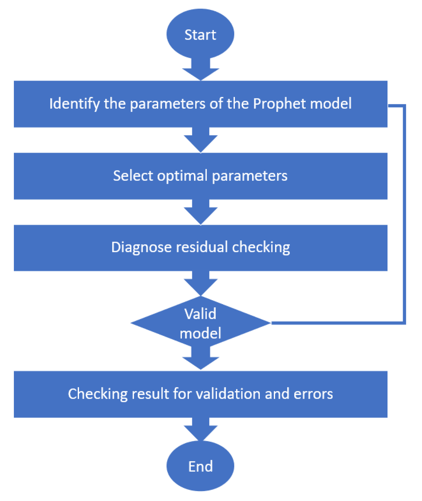
3.4. Time Series Prediction with Prophet Model

Prophet [32] is a versatile model capable of detecting trends, seasonality, missing numbers, and outliers [36]. Depending on the temporal trend, seasonality can play a crucial role in forecasting systems and profoundly influence predictions. Prophet, developed by Facebook, addresses certain challenges encountered with ARIMA [33]. Prophet operates by employing an additive model that effectively captures non-linear trends in the dataset by incorporating suitable seasonality. The visual representation of the Prophet model can be observed in Figure 3.

Given that the Prophet model operates on data patterns, intricate characteristics are derived from holidays and seasonal data. Seasonality is incorporated with considerations for daily, weekly, and yearly factors. The Prophet model utilizes time series data to represent consumption, and its data methodology can be articulated in the following manner:

$$y\left(t\right)=g\left(t\right)+s\left(t\right)+h\left(t\right)+e\left(t\right)$$

(9)

In this context, $y\left(t\right)$ represents the endogenous variable,$g\left(t\right)$ signifies the data trend function, $s\left(t\right)$ the seasonal data, $h\left(t\right)$ the holiday-based data, and $e\left(t\right)$ stands for the errors.

The trend function of the Prophet model, denoted as $g\left(t\right)$, is characterized by a piecewise linear growth model, also referred to as a saturation-growth model. However, the observed maximum load data does not exhibit a saturating growth pattern. This deviation is captured by a piecewise linear growth model described as follows:

$$g\left(t\right)=(k+{a\left(t\right)}^T\delta )t+(n+{a\left(t\right)}^T\sigma )$$

(10)

Here, $k$ represents the growth rate, $\delta$ denotes the rate adjustment, $n$ is an offset parameter, and $\sigma$ stands for the change point.

The Prophet model utilizes the Fourier series to model and predict seasonal effects. The expression of the seasonality function can be described by the following equation:

$$s\left(t\right)=\sum _{n=1}^N{a}_{n}cos\left(\frac{2\pi nt}{P}\right)+b_{n}sin\left(\frac{2\pi nt}{P}\right)$$

(11)

In Equation (12), $s\left(t\right)$ represents the seasonality function, N denotes the number of cycles used in the model; P signifies the period length of the desired time series; 2n represents the number of parameters that need to be estimated for fitting seasonality; $a_n$is the coefficient (amplitude) of the cosine of the frequency doubling of n and $b_n$ is the coefficient (amplitude) of the sinusoidal frequency doubling of n. For annual data, $P$ = 365.25, and for weekly data, P = 7.

Conversely, to integrate holidays into the model, for each holiday $i$, let $D_i$ denote the set of past and future dates for that particular holiday. We introduce an indicator function to signify whether time $t$ falls within holiday $i$, and assign a parameter $k_i$to each holiday, representing the corresponding change in the forecast. This process parallels the handling of seasonality, where we generate a matrix of regressors $Z\left(t\right)$ as discussed:

$$Z\left(t\right)=\left[1\right(t\in D_1),\cdots ,1(t\in D_L\left)\right]$$

(12)

and taking

$$h\left(t\right)=Z_{t}k$$

(13)

In Equation (13), $h\left(t\right)$ indicates holidays and $k$ indicates a corresponding change in the forecast.

3.5. Dataset

To apply the proposed model (see Section 5), a specific dataset has been built from the social network X focusing on the COVID-19 pandemic suffered in Spain. The tweets have been collected using a library programmed in R language that returns the messages (without retweets) published each day written in Spanish (“lang = es”) and within a geographical area with the center in Madrid and radius equal to 750 km (not including, therefore, the Canary Islands). The geo-referenced tweets were filtered and in the query the parameter “lang = ES” was used to filter the messages written in Spanish, finally obtaining a total set of 4,389,259 tweets. The dates considered in this study were from 23 February to 30 April, to cover the two-month lockdown.

In addition, a set of daily indicators from official sources are added; namely, the figures on deaths from the National Institute of Statistics (https://www.ine.es/dyngs/INEbase/en/categoria.htm?c=Estadistica_P&cid=1254735573175, accessed on 5 March 2024) (health indicator), the IBEX-35 stock market price data from Bolsa de Madrid (https://www.bolsasymercados.es/bme-exchange/es/Bolsa-Madrid, accessed on 5 March 2024) (economic indicator), and the data on infections provided by the National Epidemiology Center (https://cneCOVID.isciii.es/COVID19/, accessed on 5 March 2024) (health indicator). In this manner, a file is obtained that integrates various sources of information.

4. Proposed Model

A model for crisis management is proposed within the three-layer architecture based on Big Data and Artificial Intelligence [5]. In this architecture, a KDD (Knowledge Discovery in Databases) methodology is implemented (refer to Figure 4). This methodology was introduced in [37,38].

In our model, we leverage information gathered from opinions expressed on social networks (tweets) to complement official statistics, thereby enhancing our understanding of the social context. This approach is applied to a case study focused on crisis management during the initial lockdown in Spain amid the COVID-19 pandemic. The following section provides a more detailed explanation of the KDD phases that were followed:

4.1. Understanding the Application Domain

In this first phase, it is necessary to understand the underlying domain of the application to be developed, in this case monitoring sentiments in case of a health crisis. As explained in the Introduction, the objective is monitoring social feelings using information from social networks and official statistics, and how this combination of data can provide a more complete view of the social dynamics in times of health emergency in the period of lockdown in Spain due to the COVID-19 pandemic.

4.2. Creating the Dataset

In this phase, the global set of data to be used to develop the project is obtained. In our case, it is a matter of determining the optimal set of data, both those that will allow us to determine the social network sentiment, as well as those from other domains in the same period, which will allow us to improve the predictive objective and the social sentiment monitoring. It is important to obtain the data rapidly and reliably to be able to automate the data ingestion and subsequent steps.

In particular, tweets are obtained as described in Section 3.5. In the successive phases, the processes of pre-processing the data, obtaining the average sentiment for each day, and integration with the official daily frequency indicators are carried out.

4.3. Pre-Processing the Data

Basic cleaning operations are performed on the data from the previous stage, such as the elimination of noise or incorrect data detected, treatment of missing and inconsistent values, etc. In the case of social networks, techniques such as tokenization of literals, and removal of stop words, among others, are used. Other indicators differ from social network data (“indicator variables”), since they come from official statistics, and thus do not generally require a deep cleaning.

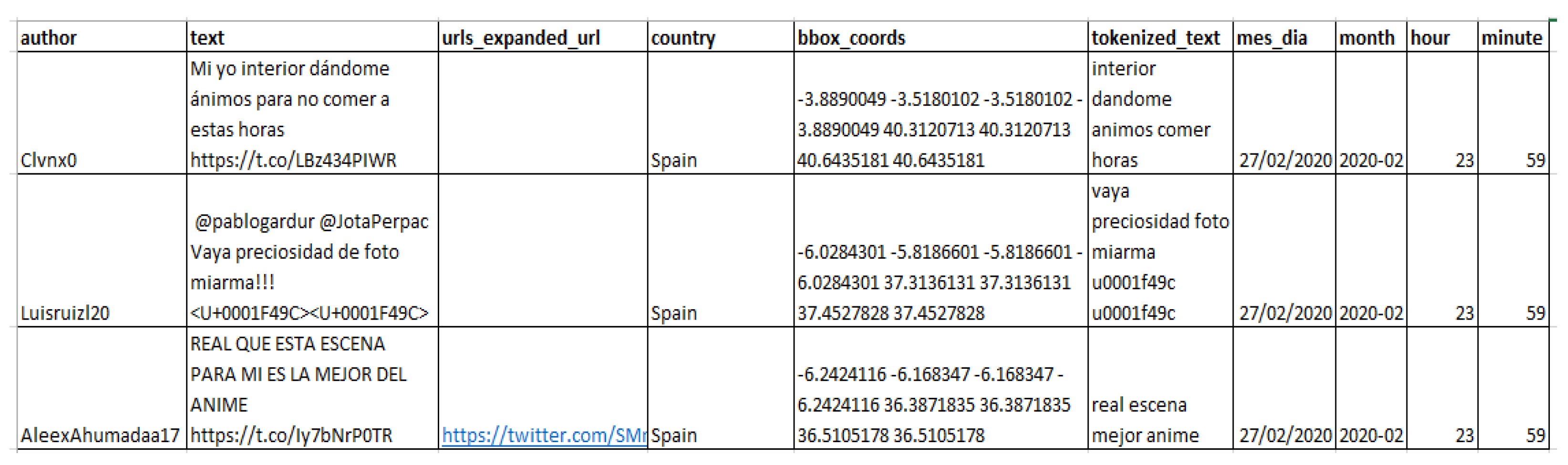
The output consists of a total of 90 variables, of which the tweet text, location, author, hashtags, and date of publication are kept. Regarding the location, two fields are of special interest: the country where the tweet is written and the coordinates, which are collected in square cells. Thus, each geographical value has 4 coordinates: two latitude and two longitude values that result in the corresponding square. The date field is converted so that you have two other new variables for the specific hour and minute when the message is posted.

The messages are then preprocessed to remove punctuation marks, graphic or web page references, words without content (stop words such as articles, prepositions, etc.), and sets of words shorter than 2 characters in length. An excerpt is shown in Figure 5.

4.4. Data Transformation

For the data from the previous stage, additional operations are carried out to obtain the sentiment and the necessary transformations for the rest of the indicators. Indicators other than social network data (“indicator variables”), coming from official statistics, do not generally require a thorough cleaning.

4.4.1. Sentiment Detection

To compute the sentiment from the posts on X, first, a training set is established. For this, a manual classification of a total of 55,841 tweets is performed. Negative, positive, and neutral sentiments will be distinguished. In total, the number of posts manually classified as positive amounted to 43,685, those classified as negative were 10,576, and neutral 1680.

The classification methods are then applied to the messages of the social network X on the dataset of 55,841 manually classified tweets, except for the Roberta model, which is sampled at 10% on the dataset and directly contrasted with the results of the manual classification.

Table 2. Mean average error for each method.

Method	MAE
Cross Validation- XGBoost	21.77
Cross Validation: SVM	22.31
Cross Validation: k-NN	25.73
Cross Validation: naïve bayes	34.71
Lexicon: ENSW	38.51
Lexicon: ISOL	66.43
Language model: RoBERTa	70.52

shows the error obtained by each method explained using the manually classified messages. Although for the case of machine learning techniques, it may seem high, and this is probably due to the bias that exists in the manual classification that has its consequences when creating the training set. It is not straightforward to determine the sentiment of certain tweets, due to the context with which they are written (images or references) and the capabilities of the classifier with no context other than the tweet itself. To determine the resulting bias, a double check of 1000 random tweets is performed, through two manual classifications by two different people independently, observing that a percentage of 29.6% are classified incorrectly. In this study, the entire dataset with a labeled sentiment is used, whereby the automatic classifiers analyzed are also expected to have a relatively high degree of error.

Consequently, it can be seen that among the best results is the option based on ENSW [25] applying Equation (1), with the already mentioned advantage of providing an exact value of the sentiment between 0 and 1 and allowing the interpretability of the algorithm used, so it will be the indicator selected to calculate the overall sentiment. To determine the sentiment of a tweet, once the sentiments suggested by each word are determined, the average sentiment of all words for each tweet is averaged.

4.4.2. Other Transformations

Once the algorithm for the calculation of the sentiment (endogenous variable) has been selected, the following transformations are carried out:

• A file is created for time series analysis, averaging the sentiment obtained for each day of the period analyzed.
• The series of exogenous variables (IBEX-35 share price, COVID-19 infections, and COVID-19 deaths related in Section 3.5) are transformed logarithmically and lagged over a period (a day) to stabilize the variance, linearize the trends, and facilitate interpretation.
• The resulting dataset has 66 observations. However, it is observed that the initial 9 observations do not provide any predictive value to the model, so they are discarded and therefore only the last 57 observations are left. Thus, a dataset TU (Twitter Universe) is obtained with the endogenous variable $s_i$ and the rest of the exogenous variables,$TU=\left\{{(u}_1,s_1,i_1,c_{1,}{d}_1),\dots ,{(u}_{\#U},s_{\#U},i_{\#U},c_{\#U,}{d}_{\#U})\right\}$, where $s_i$is the average overall sentiment, $i_i$ is the transformed variable of the IBEX-35, $c_i$ is the transformed variable for the COVID-19 infections and $d_i$ is the transformed variable for the COVID-19 deaths, for each unit $u_i$ and each day.
• As it was mentioned, the classification is not free of uncertainty, for this reason, the calculated variable of sentiment is converted into 2-tuples by applying Equation (2). In this manner, the model can better capture ambiguity by considering multiple aspects or dimensions of the utterance, can facilitate the representation of the polarity and subjectivity of an utterance, allowing a richer and more accurate classification, capturing not only the sentiment, but also the emotional intensity. A sample of the result of this process can be consulted in

  Table 3. Sample of the 2-tuple representation of the sentiment per day.

  Date	2-Tuples Sentiment
  24 February 2020	(Neu, 0.084)
  25 February 2020	(Neu, 0.078)
  26 February 2020	(Neu, 0.201)
  27 February 2020	(Pos, −0.175)

  .
• To perform the time series analysis in the next Section, Equation (3) will be applied to obtain the initial numerical value. The original transformation is applied again in Section 4.8 to interpret the results.

4.5. Selection of the Type of Machine Learning Technique to Be Applied

Depending on the objectives of the project (set in the first stage), the most appropriate machine learning techniques are selected to achieve these objectives, i.e., the prediction of time series. Several approaches are carried out to model the behavior of the sentiments on X and to determine the relationship with the other daily frequency indicators. For this purpose, the models presented in Section 3.3 are then applied.

4.5.1. Determining the Influence between Time Series

The first approach, consisting of a dynamic regression model between the sentiment variable and the regressors one-by-one, using Equations (5) and (6). The IBEX-35 economic indicator as a regressor, is presented below, and a similar proceeding applies to the rest of regressors. The ARIMA model for the sentiment time series on X is first identified. The methodology used by Box–Jenkins [33] is followed. According to the Dickey–Fuller test (p = 0.53), the hypothesis of non-stationarity in the original series is not rejected, so it is necessary to make a difference to stabilize the mean. This transformation confirms that the series is stable (p = 0.04). The simple and partial autocorrelation functions are shown to be significant only at the first lag. Therefore, the models of the type ARIMA (p, 1, q) are tested, having p, q ≤ 2. It is determined that the best model is ARIMA (0, 1, 1). Nonetheless, and looking at the behavior of the time series, it is necessary to model an anomalous behavior, such as the drop in positivity given by the confinement. This is done based on an intervention analysis, where a binary variable is added as a regressor variable; 0 before day 12 and 1 afterward. With this intervention, it is determined that the best model is still ARIMA (0, 1, 1) but with an improvement of the information criteria, both Akaike’s (AIC) and BIC, and therefore the second option is selected.

Using the pre-whitening process, the influence that sentiment has on the IBEX-35 is obtained. Using the previous model for sentiment detection on X, the series that determines the evolution of the IBEX-35 is filtered and its residuals are obtained.

Similarly, the residuals for the IBEX-35 are obtained as for the sentiment on X, verifying that they are white noise (p = 0.5 for the Ljung–Box contrast). By doing so, the cross-correlogram in Figure 6a is identified, where it can be seen that lag 1 with a positive sign is obtained as significant. This implies that the sentiment value at X affects the current IBEX-35 value one day earlier. The negative value of −8 implies that the IBEX-35 value has a certain relationship with the sentiment value of the following week. It is inferred that the sentiment on X could be used as an indicator for the IBEX-35, although it should be noted that the observation period coincides with a fall in both indicators as a consequence of the health crisis and it would therefore be necessary to have a considerably longer series to reach conclusions. The one-to-one relationship between the sentiment variable and the regressor variables is thus observed (Figure 6a–c).

The following approach consists of using the Granger test, which is a test consisting of checking whether the results of one variable serve to predict another variable, and whether it is unidirectional or bidirectional. For this, Equations (7) and (8) are applied and it is obtained (see

Table 4. Results of the Granger test.

Test	Type (Chi-Squared/F-Test)	Result	p-Value
Ho: No instantaneous causality between regressors and sentiment	Chi-squared	17.973	0.0004455
H0: COVID-19 infections and diseases do not Granger-cause sentiment	F-test	2.1343	0.03577

) that there is causality between the variables as a whole, therefore the variables that are being used, as a whole, indicate a causality in response to the sentiment variable.

As a result, a baseline is available to determine that there is a relationship between the variables of the official statistics and the one obtained from the sentiment, and the best manner of combining all the information is explored with the sentiment prediction in Section 4.5.2.

4.5.2. Time Series Prediction with Regressors

In our case, a first approach with an ARIMA model is performed with the three lagged predictor variables and with a logarithmic transformation and introducing the intervention analysis from the moment when the effects of the declaration of confinement are detected, but it is observed that when using automatic techniques for determining the ARIMA model, white noise is considered and a regression is used instead. In addition to this ARIMA model struggling to effectively incorporate predictor variables, traditional time series models face certain challenges that the Prophet model can address, such as:

• The requirement for a consistent time interval between data points is a restriction not present in the Prophet model.
• Prohibition of days with missing data (NA), a constraint that does not apply to the Prophet model.
• Complexity in handling seasonality with multiple periods, an issue that the Prophet model effortlessly manages by default.
• A more hands-on approach with a human-in-the-loop system. It provides numerous interpretable parameters that can easily be adjusted based on their forecast assumptions [39]. In contrast, the ARIMA model demands parameter tuning by an expert, whereas the Prophet model offers default settings that are easily interpretable.

Therefore, once evidence of the relationship between the predictor variables and the target is obtained (as shown in Section 4.5), the Prophet model is selected for prediction. Various models are tested to obtain the one offering the best predictive results, as explained in Section 4.6, which turns out to be the one with the series with the three predictor variables and the intervention analysis included.

4.6. Selection of the Machine Learning Models and Algorithms to Be Applied

The specific models and algorithms to be used for the project are selected considering the business requirements specified in the initial phase.

Prophet incorporates a feature for conducting time series cross-validation to assess forecast accuracy using past data. This involves identifying cutoff points in the historical data and, for each of these points, training the model using data available only up to that specific cutoff point. Subsequently, we can evaluate the forecasted values against the actual values. Our model was fit to an initial history of 40 days, and a forecast was made on a six-day horizon. This cross-validation procedure is done automatically for a range of historical cutoffs using the cross-validation function. We specify the forecast horizon (horizon = 6), the size of the initial training period (initial = 40), and the spacing between cutoff dates (period = 5). By default, the initial training period is set to three times the horizon, and cutoffs are made every half a horizon, so in our case it makes three forecasts with cutoffs between 13 April 2020 and 23 April 2020. The result of cross-validation produces a data frame containing actual values (y) and forecasted values (ŷ) for out-of-sample predictions. For each simulated forecast date and across different cutoff dates, this process is repeated. Specifically, a forecast is generated for every observed point between the cutoff and the cutoff + horizon. Subsequently, this dataset is utilized to calculate error metrics comparing ŷ and y, notably the Mean Squared Error (MSE).

4.7. Construction of the Model

By training the model, the patterns of interest sought in the project are obtained depending on the selection made in the previous stage. For this purpose, several tests are performed to find the model achieving the best predictive results using Equations of Section 3.4 and they are plotted in Figure 7 from best (green) to worst (red) predictive result for each time period.

The first (1) is the best model that includes the three transformed regressor variables and the intervention analysis discussed in Section 4.4. The next best model (2) is the model that introduces the seasonality but without other regressors and finally (3) the one that includes the three regressor variables (not transformed) and the intervention analysis.

Among the worst models is model (5) which includes the seasonality and a compact regressor that includes the information of the three predictor variables. Through an iterative trial/error process, it is decided to generate it with the regressors lagged one period and in such a manner that the difference between the values of infections and deaths exceeds a threshold (1000 and 500, respectively) and the drop of IBEX-35 index is at least 100 points. Next comes model (6) where the ranking of the sentiment variable is performed by counting the total number of values lower than the value of the observation and dividing it by the number of observations minus 1, and finally, (7) the same best model but performing a min-max transformation to the sentiment variable.

The above is evidence that Prophet is a suitable model for the time series analysis being performed and that the regressors add predictive value to the model.

4.8. Interpretation of the Knowledge Obtained

The results of the model from the previous stage are interpreted and evaluated in this phase. Thus, the previously generated knowledge is adapted for a better understanding by crisis managers through visualization techniques, monitoring, alarm generation, etc. These tools are integrated into dashboards, made with the R package shiny [40], to facilitate informed decision making, such as those in the following figures. In Figure 8, which operates as a general Dashboard, the social sentiment is interactively plotted from the desired number of observations.

From Indicator 1 (Figure 9), the emotions, the geographical distribution of sentiment, the word cloud, and the description of tweets are plotted.

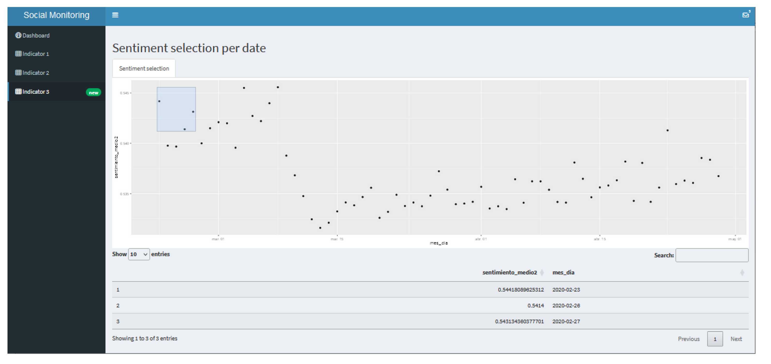
In the next Indicator (Figure 10), the prediction model results are plotted and in the last one (Figure 11), the model data can be consulted interactively.

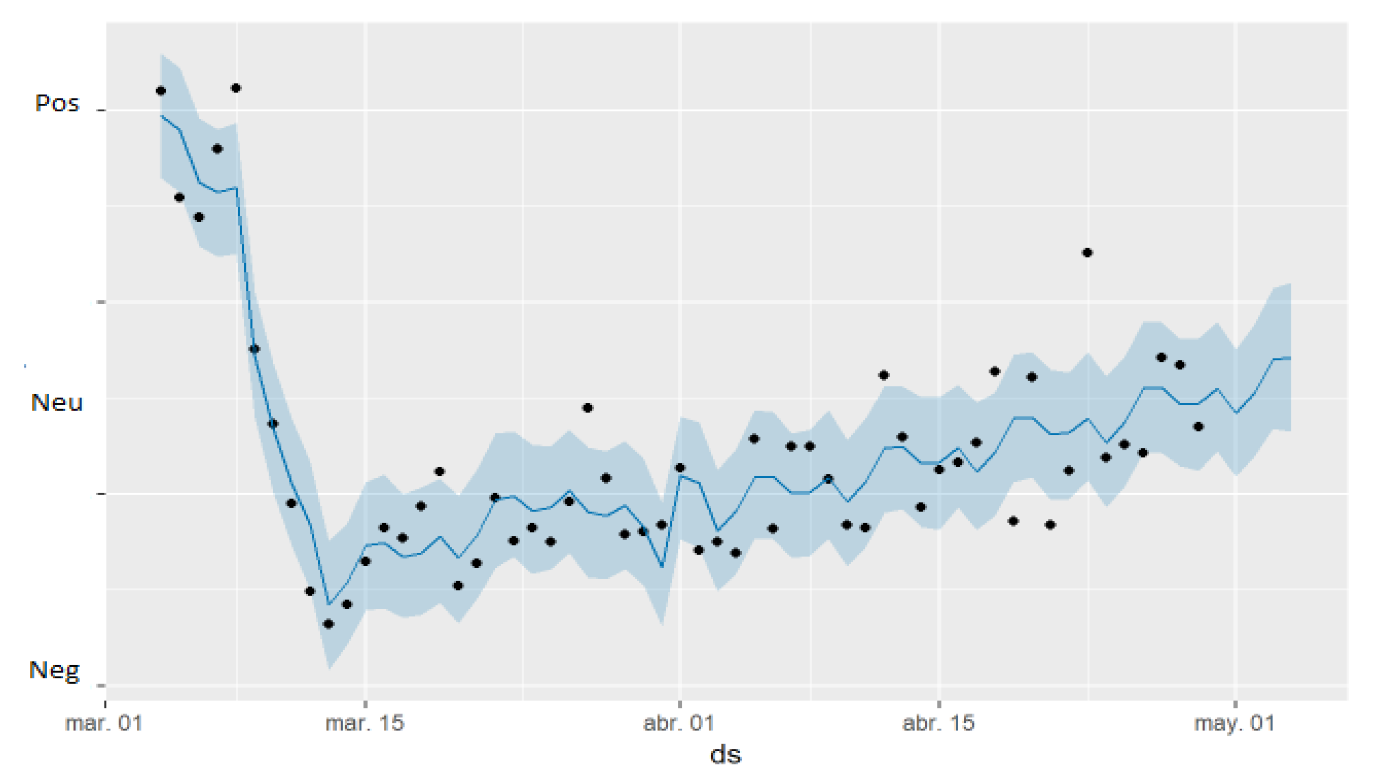
From the above dashboards, the following interpretation is derived. The model is shown graphically in Figure 12, where the points representing the sentiment and the predictive capability can be observed. The sentiment of the model is explained as discussed for the tendency. Note that the measure in this case has been presented using 2-tuples.

It is observed that, in the best of the models, the coefficient of the IBEX-35 predictor variable is a fixed term of value 1.616751 × 10⁻¹², that of COVID-19 deaths is 4.161798 × 10⁻¹², that of COVID-19 infections is −2.73167 × 10⁻¹² and other coefficients such as variable trend, additive term, extra regressors, and seasonality are incorporated. With all these coefficients, we arrive at the results of four forecasts, with cut-offs between 8 April 2020 and 23 April 2020, in

Table 5. Prophet model results at a range of 6 days.

Horizon	MSE	RMSE	MAE	MAPE
1 day	4.301527 × 10−6	0.002074012	0.001629149	0.003047079
2 days	1.635199 × 10−6	0.001278749	0.001231178	0.002296699
3 days	3.527363 × 10−6	0.001878128	0.001819491	0.003400851
4 days	2.307668 × 10−6	0.001519101	0.001246469	0.002321230
5 days	4.438489 × 10−6	0.002106772	0.001875714	0.003477166
6 days	5.618449 × 10−6	0.002370327	0.001954363	0.003652629

.

The components of the model can be seen in Figure 13.

A change in the tendency from slightly positive to sharply negative can be observed starting a few days before the official announcement of the lockdown (period 8–14 March). This is due to the uncertainty in the previous days, which aggravated the sentiment of the population, until finally the definitive announcement of the confinement took place, when a slightly positive trend started.

At the weekly seasonality level, it is observed that on Tuesday and Friday, there is a negative peak, and on Sunday and Thursday a positive peak. Concerning the rest of the regressors, greater volatility is observed during the fortnight after the announcement of the confinement.

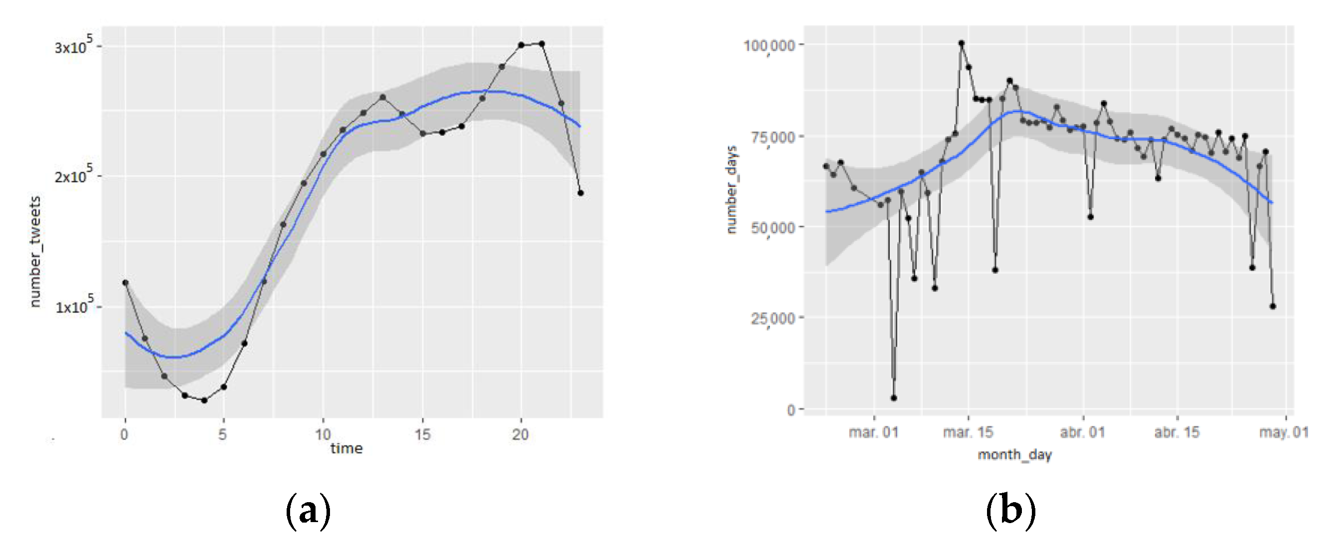
The total number of tweets obtained are distributed temporally as shown in Figure 14. The days showing the highest presence of messages correspond to important events, such as the announcement of the state of alarm on 14 March where 100,000 tweets are reached or the successive prorogations. Specifically, it is observed that during the time of the lockdown, the number of messages increased by nearly 50%. Per hour, huge differences are also appreciated, with the last part of the afternoon being the preferred time to post on the social network X.

It can be seen how the lockdown changed the words that users used most frequently, with ‘lockdown’ or ‘quarantine’ being common words that previously had not appeared. Similarly, much of the information on the posts was collected as hashtags. Figure 15 shows the most frequently used hashtags. It can be seen how the words have enormous significance and are indicative of the period analyzed.

4.9. Application of the Discovered Knowledge

In this stage, the patterns discovered are applied to the actual project according to the objectives set in the project. In our case, we found that the decision maker can make informed decisions and act consequently with the dashboard provided. Specifically, a model has been achieved that robustly predicts the sentiment of the population through social networks by relying on auxiliary information that can be available at short notice and improving the results without them. Therefore, the tools made available must be able to quickly integrate this information and provide individualized and combined information on the analyzed phenomenon, as well as descriptive information.

5. Discussion

To assess the effectiveness of this combination of data and its ability to provide a more comprehensive view of social dynamics, thereby complementing the indicators of official statistics, on the one hand, it is necessary to consider the complementarity of data sources, which is a fundamental feature of this strategy. While official data provide a solid and structured database, real-time social network information reflects the opinions and emotions of society more immediately and dynamically [41]. This combination allows the capture of events and tendencies in real-time, complementing official information that may suffer from a time lag [42].

On the other hand, monitoring social sentiment in times of emergency, such as pandemics or natural disasters, is crucial for understanding public perception and the population’s needs [43]. Social network information can provide unique insights into fear, solidarity, misinformation, and evolving attitudes during a crisis [44]. The combination with the official statistics, such as public health data, allows a more comprehensive assessment of the social impact and effectiveness of the governmental measures [45].

It is important to note that monitoring social sentiment through social networks is not free of challenges. The truthfulness of information, data privacy, and the bias inherent within social networks are significant concerns [46]. In addition, the representativeness of social network data samples is limited and may not reflect the diversity of the society [47]. These challenges have constrained us to a careful analytical approach and the use of advanced NLP techniques, such as those presented in the present study.

6. Conclusions

The proposed model provides a practical way to monitor social sentiment with information from social networks and official information, being a novel and powerful strategy for gaining a deeper understanding of social dynamics, especially in times of a health emergency.

The suggested model encompasses the following characteristics:

• Precision: the model offers an effective means to predict social sentiment accurately by analyzing both social media and official data.
• Dynamism: unlike traditional surveys, the model leverages real-time data from social media, enhancing its responsiveness and adaptability.
• Real-time Monitoring: the model enables the continuous calculation of Indicators, facilitating the implementation of a real-time privacy monitoring system.
• Flexibility: the model can be tailored to different emergency scenarios by incorporating diverse social media sources and other official statistics based on the specific nature of the situation being monitored.

For a successful implementation of the model proposed in this study, an IT architecture must be considered to support the processes described here in the various layers, in order to minimize the time required to obtain the results. In the DMSSA layer, the necessary APIs would be considered to automate the acquisition and processing of the data to be further processed, as well as the necessary storage and software infrastructure. In the IGS phase, the specific workflows process the social network data and make the predictions, and in the SA phase, to create and display the dashboards based on the data obtained in previous phases.

The combination of social network data and official information can be applied to a variety of applications, especially in assessing the effectiveness of public health campaigns and in understanding society’s response to government policies [48]. It can also be valuable for real-time decision making and risk communication.

Monitoring social sentiment through the combination of information from social networks and official information provides a more comprehensive view of social dynamics in times of emergency. This strategy allows understanding of societal attitudes, emotions, and perceptions more immediately and contextually, thus complementing official statistics indicators. Despite the inherent challenges, its potential to improve decision making and crisis management makes it a valuable tool in the field of research and public policy.

References

- Castillo-Esparcia, A.; Fernández-Souto, A.-B.; Puentes-Rivera, I. Comunicación política y COVID-19. Estrategias del Gobierno de España. Prof. Inf. 2020, 29, e290419. [Google Scholar] [CrossRef]
- Xu, Q.A.; Chang, V.; Jayne, C. A systematic review of social media-based sentiment analysis: Emerging trends and challenges. Decis. Anal. J. 2022, 3, 100073. [Google Scholar] [CrossRef]
- Alamoodi, A.; Zaidan, B.; Zaidan, A.; Albahri, O.; Mohammed, K.; Malik, R.; Almahdi, E.; Chyad, M.; Tareq, Z.; Albahri, A.; et al. Sentiment analysis and its applications in fighting COVID-19 and infectious diseases: A systematic review. Expert Syst. Appl. 2021, 167, 114155. [Google Scholar] [CrossRef]
- Biffignandi, S.; Bianchi, A.; Salvatore, C. Can Big Data provide good quality statistics? A case study on sentiment analysis on Twitter data. In Proceedings of the International Total Survey Error Workshop Duke Initiative Survey Methodol (ITSEW-DISM), Durham, NC, USA, 3 June 2018. [Google Scholar]
- Moreno, C.; González, R.A.C.; Viedma, E.H. Data and artificial intelligence strategy: A conceptual enterprise big data cloud architecture to enable market-oriented organisations. IJIMAI 2019, 5, 7–14. [Google Scholar] [CrossRef]
- Carrasco, R.A.; Blasco, M.F.; Herrera-Viedma, E. A 2-tuple fuzzy linguistic RFM model and its implementation. Procedia Comput. Sci. 2015, 55, 1340–1347. [Google Scholar] [CrossRef]
- Shu, Z.; González, R.A.C.; García-Miguel, J.P.; Sánchez-Montañés, M. Clustering using ordered weighted averaging operator and 2-tuple linguistic model for hotel segmentation: The case of TripAdvisor. Expert Syst. Appl. 2023, 213, 118922. [Google Scholar] [CrossRef]
- Bueno, I.; Carrasco, R.A.; Porcel, C.; Herrera-Viedma, E. Profiling clients in the tourism sector using fuzzy linguistic models based on 2-tuples. Procedia Comput. Sci. 2022, 199, 718–724. [Google Scholar] [CrossRef]
- Bueno, I.; Carrasco, R.A.; Ureña, R.; Herrera-Viedma, E. A business context aware decision-making approach for selecting the most appropriate sentiment analysis technique in e-marketing situations. Inf. Sci. 2022, 589, 300–320. [Google Scholar] [CrossRef]
- Kaur, S.; Kaul, P.; Zadeh, P.M. Monitoring the dynamics of emotions during COVID-19 using twitter data. Procedia Comput. Sci. 2020, 177, 423–430. [Google Scholar] [CrossRef]
- Ghazinour, K.; Matwin, S.; Sokolova, M. Monitoring and recommending privacy settings in social networks. In Proceedings of the Joint EDBT/ICDT 2013 Workshops, Genoa, Italy, 18–22 March 2013; pp. 164–168. [Google Scholar]
- Alexander, S.M.; Epstein, G.; Bodin, Ö.; Armitage, D.; Campbell, D. Participation in planning and social networks increase social monitoring in community-based conservation. Conserv. Lett. 2018, 11, e12562. [Google Scholar] [CrossRef]
- Nguyen, T.; Venkatesh, S.; Phung, D. Textual cues for online depression in community and personal settings. In Proceedings of the Advanced Data Mining and Applications: 12th International Conference, ADMA 2016, Gold Coast, QLD, Australia, 12–15 December 2016; Proceedings 12. Springer International Publishing: Berlin/Heidelberg, Germany, 2016. [Google Scholar]
- Nepali, R.K.; Wang, Y. Sonet: A social network model for privacy monitoring and ranking. In Proceedings of the 2013 IEEE 33rd International Conference on Distributed Computing Systems Workshops, Philadelphia, PA, USA, 8–11 July 2013. [Google Scholar]
- Piedrahita-Valdés, H.; Piedrahita-Castillo, D.; Bermejo-Higuera, J.; Guillem-Saiz, P.; Bermejo-Higuera, J.R.; Guillem-Saiz, J.; Sicilia-Montalvo, J.A.; Machío-Regidor, F. Vaccine hesitancy on social media: Sentiment analysis from June 2011 to April 2019. Vaccines 2021, 9, 28. [Google Scholar] [CrossRef]
- Zucco, C.; Calabrese, B.; Agapito, G.; Guzzi, P.H.; Cannataro, M. Sentiment analysis for mining texts and social networks data: Methods and tools. WIREs Data Min. Knowl. Discov. 2020, 10, e1333. [Google Scholar] [CrossRef]
- Sufi, F.K.; Khalil, I.; Sufi, F.K.; Khalil, I. Automated Disaster Monitoring From Social Media Posts Using AI-Based Location Intelligence and Sentiment Analysis. IEEE Trans. Comput. Soc. Syst. 2022, 1–11. [Google Scholar] [CrossRef]
- Tran, M.; Draeger, C.; Wang, X.; Nikbakht, A. Monitoring the well-being of vulnerable transit riders using machine learning based sentiment analysis and social media: Lessons from COVID-19. Environ. Plan. B Urban Anal. City Sci. 2023, 50, 60–75. [Google Scholar] [CrossRef]
- El Barachi, M.; AlKhatib, M.; Mathew, S.; Oroumchian, F. A novel sentiment analysis framework for monitoring the evolving public opinion in real-time: Case study on climate change. J. Clean. Prod. 2021, 312, 127820. [Google Scholar] [CrossRef]
- Madhoushi, Z.; Hamdan, A.R.; Zainudin, S. Sentiment analysis techniques in recent works. In Proceedings of the 2015 Science and Information Conference (SAI), London, UK, 28–30 July 2015. [Google Scholar]
- Benoit, K.; Watanabe, K.; Wang, H.; Nulty, P.; Obeng, A.; Müller, S.; Matsuo, A. Quanteda: An R package for the quantitative analysis of textual data. J. Open Source Softw. 2018, 3, 774. [Google Scholar] [CrossRef]
- Schütze, H.; Manning, C.D.; Raghavan, P. Introduction to Information Retrieval; Cambridge University Press: Cambridge, UK, 2008. [Google Scholar]
- Zhang, L.; Ghosh, R.; Dekhil, M.; Hsu, M.; Liu, B. Combining Lexicon-Based and Learning-Based Methods for Twitter Sentiment Analysis; HP Laboratories, Technical Report HPL-2011; HP Laboratories: Palo Alto, CA, USA, 2011; Volume 89, pp. 1–8. [Google Scholar]
- Molina-González, M.D.; Martínez-Cámara, E.; Martín-Valdivia, M.-T.; Perea-Ortega, J.M. Semantic orientation for polarity classification in Spanish reviews. Expert Syst. Appl. 2013, 40, 7250–7257. [Google Scholar] [CrossRef]
- Bradley, M.M.; Lang, P.J. Affective Norms for English Words (ANEW): Instruction Manual and Affective Ratings; Technical Report C-1; The Center for Research in Psychophysiology, University of Florida: Gainesville, FL, USA, 1999. [Google Scholar]
- Redondo, J.; Fraga, I.; Padrón, I.; Comesaña, M. The Spanish adaptation of ANEW (affective norms for English words). Behav. Res. Methods 2007, 39, 600–605. [Google Scholar] [CrossRef]
- Stadthagen-Gonzalez, H.; Imbault, C.; Pérez Sánchez, M.A.; Brysbaert, M. Norms of valence and arousal for 14,031 Spanish words. Behav. Res. Methods 2017, 49, 111–123. [Google Scholar] [CrossRef] [PubMed]
- del Castillo, P.R. A sentiment index based on Spanish tweets. BEIO Boletín Estadística Investig. Oper. 2019, 35, 130–147. [Google Scholar]
- Adoma, A.F.; Henry, N.M.; Chen, W. Comparative analyses of bert, roberta, distilbert, and xlnet for text-based emotion recognition. In Proceedings of the 2020 17th International Computer Conference on Wavelet Active Media Technology and Information Processing (ICCWAMTIP), Chengdu, China, 18–20 December 2020. [Google Scholar]
- Serrano-Guerrero, J.; Bani-Doumi, M.; Romero, F.P.; Olivas, J.A. A 2-tuple fuzzy linguistic model for recommending health care services grounded on aspect-based sentiment analysis. Expert Syst. Appl. 2024, 238, 122340. [Google Scholar] [CrossRef]
- Martinez, L.; Herrera, F. A 2-tuple fuzzy linguistic representation model for computing with words. IEEE Trans. Fuzzy Syst. 2000, 8, 746–752. [Google Scholar] [CrossRef]
- Taylor, S.J.; Letham, B. Forecasting at scale. Am. Stat. 2018, 72, 37–45. [Google Scholar] [CrossRef]
- Box, G.E.P.; Jenkins, G.M.; Reinsel, G.C.; Ljung, G.M. Time Series Analysis: Forecasting and Control; John Wiley & Sons: Hoboken, NJ, USA, 2015. [Google Scholar]
- Haugh, L.D.; Box, G.E. Identification of dynamic regression (distributed lag) models connecting two time series. J. Am. Stat. Assoc. 1977, 72, 121–130. [Google Scholar] [CrossRef]
- Granger, C.W.J. Investigating causal relations by econometric models and cross-spectral methods. Econom. J. Econom. Soc. 1969, 37, 424–438. [Google Scholar] [CrossRef]
- Huang, Y.-T.; Bai, Y.-L.; Yu, Q.-H.; Ding, L.; Ma, Y.-J. Application of a hybrid model based on the Prophet model, ICEEMDAN and multi-model optimization error correction in metal price prediction. Resour. Policy 2022, 79, 102969. [Google Scholar] [CrossRef]
- Brachman, R.J.; Anand, T. The process of knowledge discovery in databases: A first sketch. In Proceedings of the 3rd International Conference on Knowledge Discovery and Data Mining, Seattle, WA, USA, 31 July–1 August 1994. [Google Scholar]
- Fayyad, U.; Piatetsky-Shapiro, G.; Smyth, P. From data mining to knowledge discovery in databases. AI Mag. 1996, 17, 37. [Google Scholar]
- Dutt, A. Time Series Forecasting Using Machine Learning Menlo Park, CA 94025, USA. 2021. Available online: https://digital.kenyon.edu/dh_iphs_ss/6/ (accessed on 5 March 2024).
- Sievert, C. Interactive Web-Based Data Visualization with R, Plotly, and Shiny; CRC Press: Boca Raton, FL, USA, 2020. [Google Scholar]
- Gruzd, A.; Wellman, B.; Takhteyev, Y. Imagining twitter as an imagined community. Am. Behav. Sci. 2011, 55, 1294–1318. [Google Scholar] [CrossRef]
- Biancotti, C.; Rosolia, A.; Veronese, G.; Kirchner, R.; Mouriaux, F. COVID-19 and Official Statistics: A Wakeup Call? (12 February 2021). Bank of Italy Occasional Paper No. 605. Available online: https://ssrn.com/abstract=3828122 (accessed on 1 January 2024).
- Stieglitz, S.; Dang-Xuan, L. Emotions and information diffusion in social media—Sentiment of microblogs and sharing behavior. J. Manag. Inf. Syst. 2013, 29, 217–248. [Google Scholar] [CrossRef]
- Vieweg, S.; Hughes, A.L.; Starbird, K.; Palen, L. Microblogging during two natural hazards events: What twitter may contribute to situational awareness. In Proceedings of the SIGCHI Conference on Human Factors in Computing Systems, Atlanta, GA, USA, 10–15 April 2010. [Google Scholar]
- Chew, C.; Eysenbach, G. Pandemics in the age of twitter: Content analysis of tweets during the 2009 H1N1 outbreak. PLoS ONE 2010, 5, e14118. [Google Scholar] [CrossRef] [PubMed]
- Kwak, H.; Lee, C.; Park, H.; Moon, S. What is Twitter, a social network or a news media? In Proceedings of the 19th International Conference on World Wide Web, Raleigh, NC, USA, 26–30 April 2010. [Google Scholar]
- Tufekci, Z. Big questions for social media big data: Representativeness, validity and other methodological pitfalls. In Proceedings of the International AAAI Conference on Web and Social Media, Oxford, UK, 26–29 May 2014; Volume 8. No. 1. [Google Scholar]
- Signorini, A.; Segre, A.M.; Polgreen, P.M. The use of twitter to track levels of disease activity and public concern in the U.S. during the influenza A H1N1 pandemic. PLoS ONE 2011, 6, e19467. [Google Scholar] [CrossRef] [PubMed]
Figure 1.
Three-layer architecture for sentiment monitoring.
Figure 2.
Definition of the set S.
Figure 3.
Steps of the Prophet model, where the parameters can be adjusted based on the evaluation of the models.
Figure 4.
Integration of the KDD phases into the three-layer architecture.
Figure 5.
Pre-processed data, accessed on 1 January 2024.
Figure 6.
Cross-correlation function of IBEX-35 (a), COVID-19 infections (b), and deaths (c) with sentiment after pre-whitening.
Figure 7.
Better and worse results according to the Prophet model measured by MSE.
Figure 8.
Social Dashboard.
Figure 9.
Social Dashboard Indicator 1.
Figure 10.
Social Dashboard Indicator 2.
Figure 11.
Social Dashboard Indicator 3.
Figure 12.
Prediction model with the 2-tuple sentiment and the Prophet time variable (ds).
Figure 13.
Model components.
Figure 14.
Number of tweets per hour (a) and day (b).
Figure 15.
Word cloud of the most used hashtags during the lockdown.