Analysis of Shielded Harmonic and Biharmonic Systems by the Iterative Extension Method

Abstract

To describe stationary physical systems, well-known boundary problems for shielded Poisson and Sophie Germain equations are used. The obtained shielded harmonic and biharmonic systems are approximated using the finite element method and fictitiously continued. The resulting problems are solved using the developed method of iterative extensions. To expedite the convergence of this method, the relationships between physical quantities on the extension of systems and additional parameters of the iterative method are employed. The formulations of sufficient convergence conditions for the iterative process utilize interdisciplinary connections with functional analysis, applying discrete analogs of the principles of function extensions while preserving norm and class. In the algorithmic implementation of the iterative extensions method, automation is applied to control the selection of the optimal iterative parameter value during information processing. In accordance with the fictitious domain methodology, solvable problems from domains with a complex geometry are reduced to problems in a rectangle in the two-dimensional case and in a rectangular parallelepiped in the three-dimensional case. But now, in the problems being solved, the minimization of the error of the iterative processes is carried out with a norm stronger than the energy norm. Then, all relative errors are estimated from above in the used norms by terms of infinitely decreasing geometric progressions. A generalization of the developed methodology to boundary value problems for polyharmonic equations is possible.

1. Introduction

This article is dedicated to the development of a new iterative extensions method for the analysis of stationary physical systems [1,2,3,4,5,6]. The numerical solution of the biharmonic equation and similar ones, even in a square region, under the main boundary conditions has not been sufficiently mastered, and there are difficulties in solving such problems. The solution of shielded Poisson and Sophie Germain equations is considered with a mandatory presence of the Dirichlet boundary condition. Developing a method that is asymptotically optimal in terms of computational costs for solving such problems is challenging [7]. For the screened Poisson equation, such a method was obtained in [8]. This method was quite complicated, not universal, and was not developed, for example, in [9,10,11]. The work reported in [8] provides a more detailed overview of the fundamental works on the developed methodology. It is worth noting that there are a large number of approaches to solving the problems under consideration, which are not listed here. This work has a highly specialized focus on the used methodology. We can say that a new development of fictitious domain methods is proposed, for example, as in [8,12]. The considered problems have both differences and common properties. To illustrate this, it is necessary to present their classical and generalized formulations simultaneously.

Firstly, this article is devoted to the development of a new method of iterative extensions for the analysis of the screened biharmonic system [13]. A shielded biharmonic system is a mixed boundary problem for the shielded Sophie Germain equation.

$${\displaystyle \stackrel{⌣}{u}}:\hspace{0.17em}\hspace{0.17em}{\Delta }^2\stackrel{⌣}{u}={\stackrel{⌣}{f}|}_{\Omega },\hspace{0.17em}\hspace{0.17em}\Omega \subset {ℝ}^2,$$

(1)

$$\stackrel{⌣}{u}={\frac{\mathsf{\partial }\stackrel{⌣}{u}}{\mathsf{\partial }n}|}_{{\Gamma }_0}=0,\hspace{0.17em}\hspace{0.17em}\stackrel{⌣}{u}=l_1{\stackrel{⌣}{u}|}_{{\Gamma }_1}=0,\hspace{0.17em}\hspace{0.17em}\frac{\mathsf{\partial }\stackrel{⌣}{u}}{\mathsf{\partial }n}=l_2{\stackrel{⌣}{u}|}_{{\Gamma }_2}0,\hspace{0.17em}\hspace{0.17em}{l}_1\stackrel{⌣}{u}=l_2{\stackrel{⌣}{u}|}_{{\Gamma }_3}0,$$

where Ω is a bounded domain in the plane with a piecewise-smooth boundary, and $n$ is the external normal to $\mathsf{\partial }\Omega$.

$$\mathsf{\partial }\Omega =\overline{s},\hspace{0.17em}\hspace{0.17em}s={\Gamma }_0\cup {\Gamma }_1\cup {\Gamma }_2\cup {\Gamma }_3,\hspace{0.17em}\hspace{0.17em}{\Gamma }_i\cap {\Gamma }_j=\mathsf{\varnothing },\hspace{0.17em}\hspace{0.17em}i\ne j,\hspace{0.17em}\hspace{0.17em}i,j=0,1,2,3,$$

$$l_1\stackrel{⌣}{u}=\Delta \stackrel{⌣}{u}+(1-\sigma )n_1{n}_2{\stackrel{⌣}{u}}_{xy}-n_2^2{\stackrel{⌣}{u}}_{xx}-n_1^2{\stackrel{⌣}{u}}_{yy},$$

$$l_2\stackrel{⌣}{u}=\frac{\mathsf{\partial }\Delta \stackrel{⌣}{u}}{\mathsf{\partial }n}+(1-\sigma )\frac{\mathsf{\partial }}{\mathsf{\partial }s}(n_1{n}_2({\stackrel{⌣}{u}}_{yy}-{\stackrel{⌣}{u}}_{xx})+(n_1^2-n_2^2){\stackrel{⌣}{u}}_{xy}),$$

$$n_1=-\cos (n,x),\hspace{0.17em}\hspace{0.17em}{n}_2=-\cos (n,y),\hspace{0.17em}\hspace{0.17em}\sigma \in (0;\hspace{0.17em}1).$$

The previous boundary problem can be formulated as the representation of a linear functional in the form of a scalar product:

$$\stackrel{⌣}{u}\in \stackrel{⌣}{H}:\hspace{0.17em}\hspace{0.17em}[\stackrel{⌣}{u},\stackrel{⌣}{v}]=F(\stackrel{⌣}{v})\hspace{0.17em}\hspace{0.17em}\forall \stackrel{⌣}{v}\in \stackrel{⌣}{H},\hspace{0.17em}\hspace{0.17em}F\in {\stackrel{⌣}{H}}^{\prime },$$

(2)

where the space of Sobolev functions is

$$\stackrel{⌣}{H}=\stackrel{⌣}{H}(\Omega )=\left\{\stackrel{⌣}{v}\in W_2^2(\Omega ):\hspace{0.17em}\hspace{0.17em}{\left.\stackrel{⌣}{v}\right|}_{{\Gamma }_0\cup {\Gamma }_1}=0,\hspace{0.17em}\hspace{0.17em}\frac{\mathsf{\partial }\stackrel{⌣}{v}}{\mathsf{\partial }n}{|}_{{\Gamma }_0\cup {\Gamma }_2}=0\right\},$$

and the scalar product is

$$[\stackrel{⌣}{u},\stackrel{⌣}{v}]=\Lambda (\stackrel{⌣}{u},\stackrel{⌣}{v})={\displaystyle \underset{\Omega }{\int }(\sigma \Delta \stackrel{⌣}{u}\Delta \stackrel{⌣}{v}+(1-\sigma )({\stackrel{⌣}{u}}_{xx}{\stackrel{⌣}{v}}_{xx}+2{\stackrel{⌣}{u}}_{xy}{\stackrel{⌣}{v}}_{xy}+{\stackrel{⌣}{u}}_{yy}{\stackrel{⌣}{v}}_{yy}))d\Omega },$$

If $\stackrel{⌣}{f}$ —is a given function, then the linear functional is

$$F\left(\stackrel{⌣}{v}\right)=(\stackrel{⌣}{u},\stackrel{⌣}{v})={\displaystyle \underset{\Omega }{\int }\stackrel{⌣}{f}\stackrel{⌣}{v}d\Omega }.$$

Secondly, this article is devoted to the development of a new method of iterative extensions for the analysis of the screened harmonic system [14]—a mixed boundary value problem for the screened Poisson equation in the three-dimensional case:

$$u:-\Delta \stackrel{⌣}{u}+\kappa \stackrel{⌣}{u}=\stackrel{⌣}{f}{|}_{\Omega }, \Omega \subset {ℝ}^3, {\stackrel{⌣}{u}|}_{{\Gamma }_1}=0, {\frac{\mathsf{\partial }\stackrel{⌣}{u}}{\mathsf{\partial }n}|}_{{\Gamma }_2}=0,$$

(3)

where $\hspace{0.17em}\mathsf{\partial }\Omega =\hspace{0.17em}\overline{s},\hspace{0.17em}\hspace{0.17em}s={\Gamma }_1\cup {\Gamma }_2,\hspace{0.17em}\hspace{0.17em}{\Gamma }_1\cap {\Gamma }_2=\mathsf{\varnothing }$, $\kappa \in \left[0;+\infty \right)$, $\hspace{0.17em}\Omega$—is a limited region in three-dimensional space with a piecewise smooth boundary, and $n$ is the outer normal to $\hspace{0.17em}\mathsf{\partial }\Omega$.

We can formulate the previous boundary value problem as the problem of representing a linear functional in the form of a scalar product:

$$\stackrel{⌣}{u}\in \stackrel{⌣}{H}:\hspace{0.17em}\hspace{0.17em}\left[\stackrel{⌣}{u},\stackrel{⌣}{v}\right]=F(\stackrel{⌣}{v})\hspace{0.17em}\hspace{0.17em}\forall \stackrel{⌣}{v}\in \stackrel{⌣}{H},$$

(4)

where the Sobolev space is

$$\stackrel{⌣}{H}=\stackrel{⌣}{H}(\Omega )=\left\{\stackrel{⌣}{v}\in W_2^1(\Omega ):\hspace{0.17em}\hspace{0.17em}{\left.\stackrel{⌣}{v}\right|}_{{\Gamma }_1}=0\right\},$$

and the scalar product is

$$\left[\stackrel{⌣}{u},\stackrel{⌣}{v}\right]=A(\stackrel{⌣}{u},\stackrel{⌣}{v})={\displaystyle \underset{\Omega }{\int }({\stackrel{⌣}{u}}_x{\stackrel{⌣}{v}}_x+{\stackrel{⌣}{u}}_y{\stackrel{⌣}{v}}_y+{\stackrel{⌣}{u}}_z{\stackrel{⌣}{v}}_z+\kappa \stackrel{⌣}{u}\stackrel{⌣}{v})d\Omega },$$

and if $\stackrel{⌣}{f}$ is the given function, then the linear functional is

$$F(\stackrel{⌣}{v})=\left(\stackrel{⌣}{u},\stackrel{⌣}{v}\right)={\displaystyle \underset{\Omega }{\int }\stackrel{⌣}{f}\stackrel{⌣}{v}d\Omega }.$$

Due to the universality of the formulations of the above problems, universal methods for solving them are being developed. In the method of iterative extensions, the computational costs are asymptotically optimal, i.e., the number of operations is of the order of the number of unknowns in the resulting systems of linear algebraic equations, if at each step of the applied iterative processes, known marching methods are used, for example, from [1].

2. Analysis of Shielded Biharmonic System

Let us consider the shielded biharmonic system in a variational form:

$${\stackrel{⌣}{u}}_{\omega }\in {\stackrel{⌣}{H}}_{\omega }:\hspace{0.17em}\hspace{0.17em}{\Lambda }_{\omega }({\stackrel{⌣}{u}}_{\omega },{\stackrel{⌣}{v}}_{\omega })=F_{\omega }({\stackrel{⌣}{v}}_{\omega })\hspace{0.17em}\hspace{0.17em}\forall {\stackrel{⌣}{v}}_{\omega }\in {\stackrel{⌣}{H}}_{\omega },\hspace{0.17em}\hspace{0.17em}{F}_{\omega }\in {{\stackrel{⌣}{H}}^{\prime }}_{\omega },\hspace{0.17em}\hspace{0.17em}\omega \in \left\{1,\hspace{0.17em}\hspace{0.17em}{\rm I}{\rm I}\right\},\hspace{0.17em}\hspace{0.17em}{\Omega }_{\omega }\subset {ℝ}^2,$$

(5)

where the right-hand side of the problem, if ${\stackrel{⌣}{f}}_1\in L_2({\Omega }_1)$ is a given function, is given as

$$F_{\omega }({\stackrel{⌣}{v}}_{\omega })={\displaystyle \underset{{\Omega }_{\omega }}{\int }{\stackrel{⌣}{f}}_{\omega }{\stackrel{⌣}{v}}_{\omega }d{\Omega }_{\omega }\hspace{0.17em}\hspace{0.17em}\forall {\stackrel{⌣}{v}}_{\omega }\hspace{0.17em}\in {\stackrel{⌣}{H}}_{\omega },\hspace{0.17em}\hspace{0.17em}{\stackrel{⌣}{f}}_{{\rm I}{\rm I}}=0,}$$

where the space of Sobolev functions is

$${\stackrel{⌣}{H}}_{\omega }={\stackrel{⌣}{H}}_{\omega }({\Omega }_{\omega })=\left\{{\stackrel{⌣}{v}}_{\omega }\in W_2^2({\Omega }_{\omega }):\hspace{0.17em}\hspace{0.17em}{\left.{\stackrel{⌣}{v}}_{\omega }\right|}_{{\Gamma }_{\omega ,0}\cup {\Gamma }_{\omega ,1}}=0,\hspace{0.17em}\hspace{0.17em}\frac{\mathsf{\partial }{\stackrel{⌣}{v}}_{\omega }}{\mathsf{\partial }{n}_{\omega }}{|}_{{\Gamma }_{\omega ,0}\cup {\Gamma }_{\omega ,2}}=0\right\},$$

on a flat, bounded domain ${\Omega }_{\omega }$ with a boundary:

$$\mathsf{\partial }{\Omega }_{\omega }={\overline{s}}_{\omega },\hspace{0.17em}\hspace{0.17em}{s}_{\omega }={\Gamma }_{\omega ,0}\cup {\Gamma }_{\omega ,1}\cup {\Gamma }_{\omega ,2}\cup {\Gamma }_{\omega ,3},$$

$${\Gamma }_{\omega ,i}\cap {\Gamma }_{\omega ,j}=\mathsf{\varnothing }, \mathrm{if} i\ne j, i,j=0,1,2,3,$$

and $n_{\omega }-$ is the external normal to ${\Omega }_{\omega }$, and the scalar product is

$${\Lambda }_{\omega }({\stackrel{⌣}{u}}_{\omega },{\stackrel{⌣}{v}}_{\omega })={\displaystyle \underset{{\Omega }_{\omega }}{\int }({\sigma }_{\omega }\Delta {\stackrel{⌣}{u}}_{\omega }\Delta {\stackrel{⌣}{v}}_{\omega }+(1-{\sigma }_{\omega })({\stackrel{⌣}{u}}_{\omega xx}{\stackrel{⌣}{v}}_{\omega xx}+2{\stackrel{⌣}{u}}_{\omega xy}{\stackrel{⌣}{v}}_{\omega xy}+{\stackrel{⌣}{u}}_{\omega yy}{\stackrel{⌣}{v}}_{\omega yy})+a_{\omega }{\stackrel{⌣}{u}}_{\omega }{\stackrel{⌣}{v}}_{\omega })d{\Omega }_{\omega }},$$

where coefficient $a_{\omega }\in \left[0;\hspace{0.17em}+\infty \right),$ and coefficient ${\sigma }_{\omega }\in (0;\hspace{0.17em}1)$. When considering $\omega =1,\hspace{0.17em}\hspace{0.17em}{a}_1\ge 0,\hspace{0.17em}\hspace{0.17em}{\Gamma }_{1,0}\hspace{0.17em}\ne \mathsf{\varnothing }$, the solved problem of the shielded biharmonic system is examined. When considering $\omega ={\rm I}{\rm I},\hspace{0.17em}\hspace{0.17em}{a}_{{\rm I}{\rm I}}\ge 0$, a fictitious problem of the shielded biharmonic system is examined.

The extended shielded biharmonic system is provided as follows:

$$\stackrel{⌣}{u}\hspace{0.17em}\in \stackrel{⌣}{V}:\hspace{0.17em}\hspace{0.17em}\hspace{0.17em}{\Lambda }_1(\stackrel{⌣}{u},I_1\stackrel{⌣}{v})+{\Lambda }_{{\rm I}{\rm I}}(\stackrel{⌣}{u},\stackrel{⌣}{v})=F_1(I_1\stackrel{⌣}{v})\hspace{0.17em}\hspace{0.17em}\forall \stackrel{⌣}{v}\in \stackrel{⌣}{V},$$

(6)

where the extended solution space of the considered extended problem is the Sobolev space:

$$\stackrel{⌣}{V}=\stackrel{⌣}{V}(\Pi )=\left\{\stackrel{⌣}{v}\in W_2^2(\Pi ):\hspace{0.17em}\hspace{0.17em}{\left.\stackrel{⌣}{v}\right|}_{{\Gamma }_0\cup {\Gamma }_1}=0,\hspace{0.17em}\hspace{0.17em}{\left.\frac{\mathsf{\partial }\stackrel{⌣}{v}}{\mathsf{\partial }n}\right|}_{{\Gamma }_0\cup {\Gamma }_2}=0\right\},$$

and the regions ${\Omega }_1,\hspace{0.17em}\hspace{0.17em}{\Omega }_{{\rm I}{\rm I}}$ are such that ${\overline{\Omega }}_1\cup {\overline{\Omega }}_{{\rm I}{\rm I}}=\overline{\Pi },\hspace{0.17em}\hspace{0.17em}{\Omega }_1\cap {\Omega }_{{\rm I}{\rm I}}=\mathsf{\varnothing },$ and the boundary of the region $\mathit{\Pi }$ also consists of the closure of the unions of open non-intersecting parts.

$$\mathsf{\partial }\Pi =\overline{s},\hspace{0.17em}\hspace{0.17em}s={\Gamma }_0\cup {\Gamma }_1\cup {\Gamma }_2\cup {\Gamma }_3,\hspace{0.17em}\hspace{0.17em}{\Gamma }_i\cap {\Gamma }_j=\mathsf{\varnothing },\hspace{0.17em}\hspace{0.17em}i\ne j,\hspace{0.17em}\hspace{0.17em}i,j=0,1,2,3,$$

And the non-empty intersection of the boundary of the first region and the boundary of the second region is the closure of the intersection of the corresponding parts of the boundaries of these regions:

$$\mathsf{\partial }{\Omega }_1\cap \mathsf{\partial }{\Omega }_{{\rm I}{\rm I}}=\overline{S},\hspace{0.17em}\hspace{0.17em}S={\Gamma }_{1,0}\cap {\Gamma }_{{\rm I}{\rm I},3}\ne \mathsf{\varnothing },$$

where $n$ is the external normal to $\mathsf{\partial }\Pi$.

The extended solution space contains a subspace of solutions for the extended problem.

$${\stackrel{⌣}{V}}_1={\stackrel{⌣}{V}}_1(\Pi )=\left\{{\stackrel{⌣}{v}}_1\in \stackrel{⌣}{V}:\hspace{0.17em}\hspace{0.17em}{\left.{\stackrel{⌣}{v}}_1\right|}_{\Pi \backslash {\Omega }_1}=0\right\}.$$

Arbitrary projection operators from the extended space to the subspace of solutions for the extended problem are used in the extended problem:

$$I_1:\stackrel{⌣}{V}\mapsto {\stackrel{⌣}{V}}_1,\hspace{0.17em}\hspace{0.17em}{\stackrel{⌣}{V}}_1=\mathrm{i}\mathrm{m}{I}_1,\hspace{0.17em}\hspace{0.17em}{I}_1=I_1^2.$$

The extended shielded biharmonic system is considered in a finite-dimensional subspace of the Sobolev space. Parabolic finite elements are used for approximation. The discretization of the extended shielded biharmonic system is analyzed when

$$\Pi =(0;b_1)\times (0;b_2),{\Gamma }_0=\mathsf{\varnothing },\hspace{0.17em}\hspace{0.17em}{\Gamma }_1=\left\{b_1\right\}\times (0;b_2)\cup (0;b_1)\times \left\{b_2\right\},$$

$${\Gamma }_2=\left\{0\right\}\times (0;b_2)\cup (0;b_1)\times \left\{0\right\},\hspace{0.17em}\hspace{0.17em}{\Gamma }_3=\mathsf{\varnothing },\hspace{0.17em}\hspace{0.17em}{b}_1,b_2\in (0;+\infty ).$$

A grid is defined in a rectangular domain with nodes:

$$(x_i;y_j)=\left((i-1,5)h_1;(j-1,5)h_2\right),$$

$$h_1=b_1/(m-1,5),\hspace{0.17em}\hspace{0.17em}{h}_2=b_2/(n-1,5),\hspace{0.17em}\hspace{0.17em}i=1,2,\dots ,m,\hspace{0.17em}\hspace{0.17em}j=1,2,\dots ,n,\hspace{0.17em}\hspace{0.17em}m-2,n-2\in \mathbb{N}.$$

Grid functions are introduced on the set of nodes of the introduced grid:

$$v_{i,j}=v(x_i;y_j)\in ℝ,\hspace{0.17em}\hspace{0.17em}i=1,2,\dots ,m,\hspace{0.17em}\hspace{0.17em}j=1,2,\dots ,n,\hspace{0.17em}\hspace{0.17em}m-2,n-2\in \mathbb{N}.$$

Grid functions are completed using parabolic basis functions.

$${\Phi }^{i,j}(x;y)={\Psi }^{1,i}(x){\Psi }^{2,j}(y),\hspace{0.17em}\hspace{0.17em}i=2,\dots ,m-1,\hspace{0.17em}\hspace{0.17em}j=2,\dots ,n-1,\hspace{0.17em}\hspace{0.17em}m-2,n-2\in \mathbb{N},$$

$${\Psi }^{1,i}(x)=[2/i]\Psi (x/h_1-i+4)+\Psi (x/h_1-i+3)-[(i+1)/m]\Psi (x/h_1-i+1),\hspace{0.17em}$$

$${\Psi }^{2,j}(y)=[2/j]\Psi (y/h_2-j+4)+\Psi (y/h_2-j+3)+[(j+1)/n]\Psi (y/h_2-j+1),\hspace{0.17em}$$

$$\Psi (z)=\left\{\begin{array}{c}0.5z^2,\\ -z^2+3z-1.5,\\ 0.5z^2-3z-4.5,\\ 0,\end{array}\right.\hspace{0.17em}\hspace{0.17em}\begin{array}{c}z\in [0;1],\\ z\in [1;2],\\ z\in [2;3],\\ z\hspace{0.17em}\hspace{0.17em}\notin (0;3).\end{array}$$

It is assumed that the basis functions outside the rectangular domain are zero.

$${\Phi }^{i,j}(x;y)=0,\hspace{0.17em}\hspace{0.17em}(x;y)\notin \Pi ,\hspace{0.17em}\hspace{0.17em}i=2,\dots ,m-1,\hspace{0.17em}\hspace{0.17em}j=2,\dots ,n-1,\hspace{0.17em}\hspace{0.17em}m-2,n-2\in \mathbb{N}.$$

Linear combinations of basis functions are used, which define a finite-dimensional subspace in the extended solution space:

$$\tilde{V}=\left\{\tilde{v}={\displaystyle \sum _{i=2}^{m-1}{\displaystyle \sum _{j=2}^{n-1}{v}_{i,j}{\Phi }^{i,j}(x;y)}}\right\}\subset \stackrel{⌣}{V}.$$

The extended system is considered in Euclidean space. After approximation, the extended system problem is formulated in matrix form as a system of linear algebraic equations. When approximating the problem for the extended system using a finite-dimensional subspace, a system of equations is obtained.

$$\overline{u}\hspace{0.17em}\in {ℝ}^N:\hspace{0.17em}\hspace{0.17em}\hspace{0.17em}B\overline{u}=\overline{f},\hspace{0.17em}\hspace{0.17em}\overline{f}\in {ℝ}^N.$$

(7)

It is assumed that the projection operator on the solution space of the extended problem zeros the coefficients of the basis functions whose supports are not entirely contained in the first region. The extended system problem in matrix form is obtained by defining the extended matrix and the extended right-hand side of the system.

$$\begin{gathered} 〈B\overline{u},\overline{v}〉\hspace{0.17em}\hspace{0.17em}={\Lambda }_1(\tilde{u},I_1\tilde{v})+{\Lambda }_{{\rm I}{\rm I}}(\tilde{u},\tilde{v})\hspace{0.17em}\hspace{0.17em}\forall \tilde{u},\tilde{v}\in \tilde{V},\hspace{0.17em}\hspace{0.17em}〈\overline{f},\overline{v}〉\hspace{0.17em}=F_1(I_1\tilde{v})\hspace{0.17em}\hspace{0.17em}\forall \tilde{v}\in \tilde{V}, \\ 〈\overline{f},\overline{v}〉\hspace{0.17em}=(\overline{f},\overline{v})h_1{h}_2=\overline{f}\hspace{0.17em}\overline{v}{h}_1{h}_2,\hspace{0.17em}\hspace{0.17em}\overline{v}=(v_1,v_2,\dots ,v_N{)}^{\prime }\in {ℝ}^N,\hspace{0.17em}N=\hspace{0.17em}(m-2)(n-2). \end{gathered}$$

In this case, the first basis functions, whose supports are entirely contained in the first region, are numbered first. Then, the basis functions, whose supports intersect the boundary of the first region and the second region together, are numbered. The numbering ends with the basis functions, whose supports are entirely contained in the second region. With this numbering, the resulting vectors have the following form:

$$\overline{v}=({{\overline{v}}_1}^{\prime },\hspace{0.17em}{{\overline{v}}_2}^{\prime },\hspace{0.17em}{{\overline{v}}_3}^{\prime }{)}^{\prime },\hspace{0.17em}\hspace{0.17em}\overline{u}=(\hspace{0.17em}{{\overline{u}}_1}^{\prime },\hspace{0.17em}\hspace{0.17em}{\overline{0}}^{\prime },\hspace{0.17em}\hspace{0.17em}{\overline{0}}^{\prime }{)}^{\prime },\hspace{0.17em}\hspace{0.17em}\hspace{0.17em}\overline{f}=({{\overline{f}}_1}^{\prime },\hspace{0.17em}\hspace{0.17em}{\overline{0}}^{\prime },\hspace{0.17em}\hspace{0.17em}{\overline{0}}^{\prime }{)}^{\prime }.$$

The matrix has a well-known structure:

$$B=\left[\begin{array}{ccc}{\Lambda }_{11}& {\Lambda }_{12}& 0\\ 0& {\Lambda }_{02}& {\Lambda }_{23}\\ 0& {\Lambda }_{32}& {\Lambda }_{33}\end{array}\right].$$

The extended problem is solved in matrix form:

$$B\overline{u}=\overline{f},\hspace{0.17em}\hspace{0.17em}\left[\begin{array}{ccc}{\Lambda }_{11}& {\Lambda }_{12}& 0\\ 0& {\Lambda }_{02}& {\Lambda }_{23}\\ 0& {\Lambda }_{32}& {\Lambda }_{33}\end{array}\right]\left[\begin{array}{c}{\overline{u}}_1\\ \overline{0}\\ \overline{0}\end{array}\right]=\left[\begin{array}{c}{\overline{f}}_1\\ \overline{0}\\ \overline{0}\end{array}\right].$$

This solution is the matrix form of the original problem, and this is the zero solution of the fictitious problem in matrix form:

$${\Lambda }_{11}{\overline{u}}_1={\overline{f}}_1,\hspace{0.17em}\hspace{0.17em}\left[\begin{array}{cc}{\Lambda }_{02}& {\Lambda }_{23}\\ {\Lambda }_{32}& {\Lambda }_{33}\end{array}\right]\hspace{0.17em}\hspace{0.17em}\left[\begin{array}{c}{\overline{u}}_2\\ {\overline{u}}_3\end{array}\right]=\left[\begin{array}{c}\overline{0}\\ \overline{0}\end{array}\right],\hspace{0.17em}\hspace{0.17em}\left[\begin{array}{c}{\overline{u}}_2\\ {\overline{u}}_3\end{array}\right]=\left[\begin{array}{c}\overline{0}\\ \overline{0}\end{array}\right].$$

Matrices generated by scalar products are specified:

$$〈{\Lambda }_{{\rm I}}\overline{u},\overline{v}〉\hspace{0.17em}\hspace{0.17em}={\Lambda }_1(\tilde{u},\tilde{v}),\hspace{0.17em}\hspace{0.17em}〈{\Lambda }_{{\rm I}{\rm I}}\overline{u},\overline{v}〉\hspace{0.17em}\hspace{0.17em}={\Lambda }_{{\rm I}{\rm I}}(\tilde{u},\tilde{v})\hspace{0.17em}\hspace{0.17em}\forall \tilde{u},\tilde{v}\in \tilde{V}.$$

These matrices have the following structure:

$${\Lambda }_{{\rm I}}=\left[\begin{array}{ccc}{\Lambda }_{11}& {\Lambda }_{12}& 0\\ {\Lambda }_{21}& {\Lambda }_{20}& 0\\ 0& 0& 0\end{array}\right],\hspace{0.17em}\hspace{0.17em}{\Lambda }_{{\rm I}{\rm I}}=\left[\begin{array}{ccc}0& 0& 0\\ 0& {\Lambda }_{02}& {\Lambda }_{23}\\ 0& {\Lambda }_{32}& {\Lambda }_{33}\end{array}\right].$$

A subspace of vectors is introduced:

$${\overline{V}}_1=\left\{\overline{v}=({{\overline{v}}_1}^{\prime },{{\overline{v}}_2}^{\prime },{{\overline{v}}_3}^{\prime }{)}^{\prime }\in {ℝ}^N:\hspace{0.17em}\hspace{0.17em}{\overline{v}}_2=\overline{0},\hspace{0.17em}\hspace{0.17em}{\overline{v}}_3=\overline{0}\right\}.$$

Additionally, a subspace of vectors is defined:

$${\overline{V}}_2=\left\{\overline{v}=({{\overline{v}}_1}^{\prime },{{\overline{v}}_2}^{\prime },{{\overline{v}}_3}^{\prime }{)}^{\prime }\in {ℝ}^N:\hspace{0.17em}\hspace{0.17em}{\Lambda }_{11}{\overline{v}}_1+{\Lambda }_{12}{\overline{v}}_2=\overline{0},\hspace{0.17em}\hspace{0.17em}{\Lambda }_{32}{\overline{v}}_2+{\Lambda }_{33}{\overline{v}}_3=\overline{0}\right\}.$$

An asymptotically optimal analysis of the extended system is carried out based on the iterative extensions method [13]. For solving problem (7), a new iterative extensions method is used. The extended matrix is defined as the sum of the first matrix and the second matrix multiplied by a positive parameter.

$$\begin{gathered} C={\Lambda }_{{\rm I}}+\gamma {\Lambda }_{{\rm I}{\rm I}},\hspace{0.17em} \\ \hspace{0.17em}\left[\begin{array}{ccc}{C}_{11}& C_{12}& 0\\ C_{21}& C_{22}& C_{23}\\ 0& C_{32}& C_{33}\end{array}\right]=\left[\begin{array}{ccc}{\Lambda }_{11}& {\Lambda }_{12}& 0\\ {\Lambda }_{21}& {\Lambda }_{20}& 0\\ 0& 0& 0\end{array}\right]+\gamma \left[\begin{array}{ccc}0& 0& 0\\ 0& {\Lambda }_{02}& {\Lambda }_{23}\\ 0& {\Lambda }_{32}& {\Lambda }_{33}\end{array}\right],\hspace{0.17em}\hspace{0.17em}\gamma \in (0;+\infty ). \end{gathered}$$

It is assumed that the continuation conditions are satisfied.

$$\begin{gathered} \exists {\gamma }_1\in (0;+\infty ),\hspace{0.17em}\hspace{0.17em}{\gamma }_2\in [{\gamma }_1;+\infty ):\hspace{0.17em}\hspace{0.17em}{\gamma }_1^2〈C{\overline{v}}_2,C{\overline{v}}_2〉\le 〈{\Lambda }_{{\rm I}{\rm I}}{\overline{v}}_2,{\Lambda }_{{\rm I}{\rm I}}{\overline{v}}_2〉\le {\gamma }_2^2〈C{\overline{v}}_2,C{\overline{v}}_2〉\hspace{0.17em}\hspace{0.17em}\forall {\overline{v}}_2\in {\overline{V}}_2, \\ \exists \alpha \in (0;+\infty ):\hspace{0.17em}\hspace{0.17em}〈{\Lambda }_{{\rm I}}{\overline{v}}_2,{\Lambda }_{{\rm I}}{\overline{v}}_2〉\le {\alpha }^2〈{\Lambda }_{{\rm I}{\rm I}}{\overline{v}}_2,{\Lambda }_{{\rm I}{\rm I}}{\overline{v}}_2〉\hspace{0.17em}\hspace{0.17em}\forall {\overline{v}}_2\in {\overline{V}}_2. \end{gathered}$$

The iterative extensions method is a generalization of the method of fictitious components, where additional parameters are used in choosing the extended matrix, and the iterative parameters are chosen based on the method of minimal residuals.

$${\overline{u}}^k\hspace{0.17em}\in {ℝ}^N:\hspace{0.17em}\hspace{0.17em}\hspace{0.17em}C({\overline{u}}^k-{\overline{u}}^{k-1})=-{\tau }_{k-1}(B{\overline{u}}^{k-1}-\overline{f}),\hspace{0.17em}\hspace{0.17em}k\in \mathbb{N},$$

(8)

$$\forall {\overline{u}}^0\hspace{0.17em}\in {\overline{V}}_1,\hspace{0.17em}\hspace{0.17em}\gamma >\alpha ,\hspace{0.17em}\hspace{0.17em}{\tau }_0=1,\hspace{0.17em}\hspace{0.17em}{\tau }_{k-1}=〈{\overline{r}}^{k-1},{\overline{\eta }}^{k-1}〉/〈{\overline{\eta }}^{k-1},{\overline{\eta }}^{k-1}〉,\hspace{0.17em}\hspace{0.17em}k\in \hspace{0.17em}\mathbb{N}\backslash \left\{1\right\},$$

where, to calculate the iterative parameters, residuals, corrections equivalent to residuals are successively calculated.

$${\overline{r}}^{k-1}=B{\overline{u}}^{k-1}-\overline{f},\hspace{0.17em}\hspace{0.17em}{\overline{w}}^{k-1}=C^{-1}{\overline{r}}^{k-1},\hspace{0.17em}\hspace{0.17em}{\overline{\eta }}^{k-1}=B{\overline{w}}^{k-1},\hspace{0.17em}\hspace{0.17em}k\in \mathbb{N}.$$

A norm generated by the extended matrix is defined as

$$\hspace{0.17em}{‖\overline{v}‖}_{C^2}=\sqrt{〈C^2\overline{v},\overline{v}〉}\hspace{0.17em}\hspace{0.17em}\hspace{0.17em}\forall \overline{v}\in {ℝ}^N.$$

Theorem 1. 

For the iterative extensions method (8) in the analysis of the shielded biharmonic system, a convergence estimate holds:

$${‖{\overline{u}}^k-\overline{u}‖}_{C^2}\le \epsilon {‖{\overline{u}}^0-\overline{u}‖}_{C^2},\hspace{0.17em}\hspace{0.17em}\epsilon =2({\gamma }_2/{\gamma }_1)({\alpha /\gamma )}^{k-1},\hspace{0.17em}\hspace{0.17em}k\in \mathbb{N}.$$

An algorithm implementing the iterative extensions method for solving the extended system problem in Euclidean space is presented. The method of minimal residuals is applied in choosing the iterative parameters [15].

I. An initial approximation and an iterative parameter are chosen.

$$\forall {\overline{u}}^0\in {\overline{V}}_1,\hspace{0.17em}\hspace{0.17em}{\tau }_0=1.$$

II. The residual is found.

$${\overline{r}}^{k-1}=B{\overline{u}}^{k-1}-\overline{f},k\in N.$$

III. The square of the norm of the absolute error is calculated.

$${{\rm E}}_{k-1}=〈{\overline{r}}^{k-1},{\overline{r}}^{k-1}〉,\hspace{0.17em}\hspace{0.17em}k\hspace{0.17em}\in \mathbb{N}.$$

IV. The correction is found.

$${\overline{w}}^{k-1}:\hspace{0.17em}\hspace{0.17em}C{\overline{w}}^{k-1}={\overline{r}}^{k-1},\hspace{0.17em}\hspace{0.17em}k\in \mathbb{N}.$$

V. The equivalent residual is found.

$${\overline{\eta }}^{k-1}=B{\overline{w}}^{k-1},\hspace{0.17em}\hspace{0.17em}k\in \mathbb{N}\backslash \left\{1\right\}.$$

VI. The optimal value of the iterative parameter is found.

$${\tau }_{k-1}=〈{\overline{r}}^{k-1},{\overline{\eta }}^{k-1}〉/〈{\overline{\eta }}^{k-1},{\overline{\eta }}^{k-1}〉,\hspace{0.17em}\hspace{0.17em}k\in \mathbb{N}\backslash \left\{1\right\}\hspace{0.17em}\hspace{0.17em}.$$

VII. The next approximation is found.

$${\overline{u}}^k={\overline{u}}^{k-1}-{\tau }_{k-1}{\overline{w}}^{k-1},\hspace{0.17em}\hspace{0.17em}k\in \mathbb{N}.$$

VIII. The termination criterion for iterations is checked with formulas based on a specified estimate of the relative error.

$${{\rm E}}_{k-1}\le {{\rm E}}^2{{\rm E}}_0,\hspace{0.17em}\hspace{0.17em}k\in \mathbb{N}\backslash \left\{1\right\},\hspace{0.17em}\hspace{0.17em}{\rm E}\in (0;\hspace{0.17em}\hspace{0.17em}1).$$

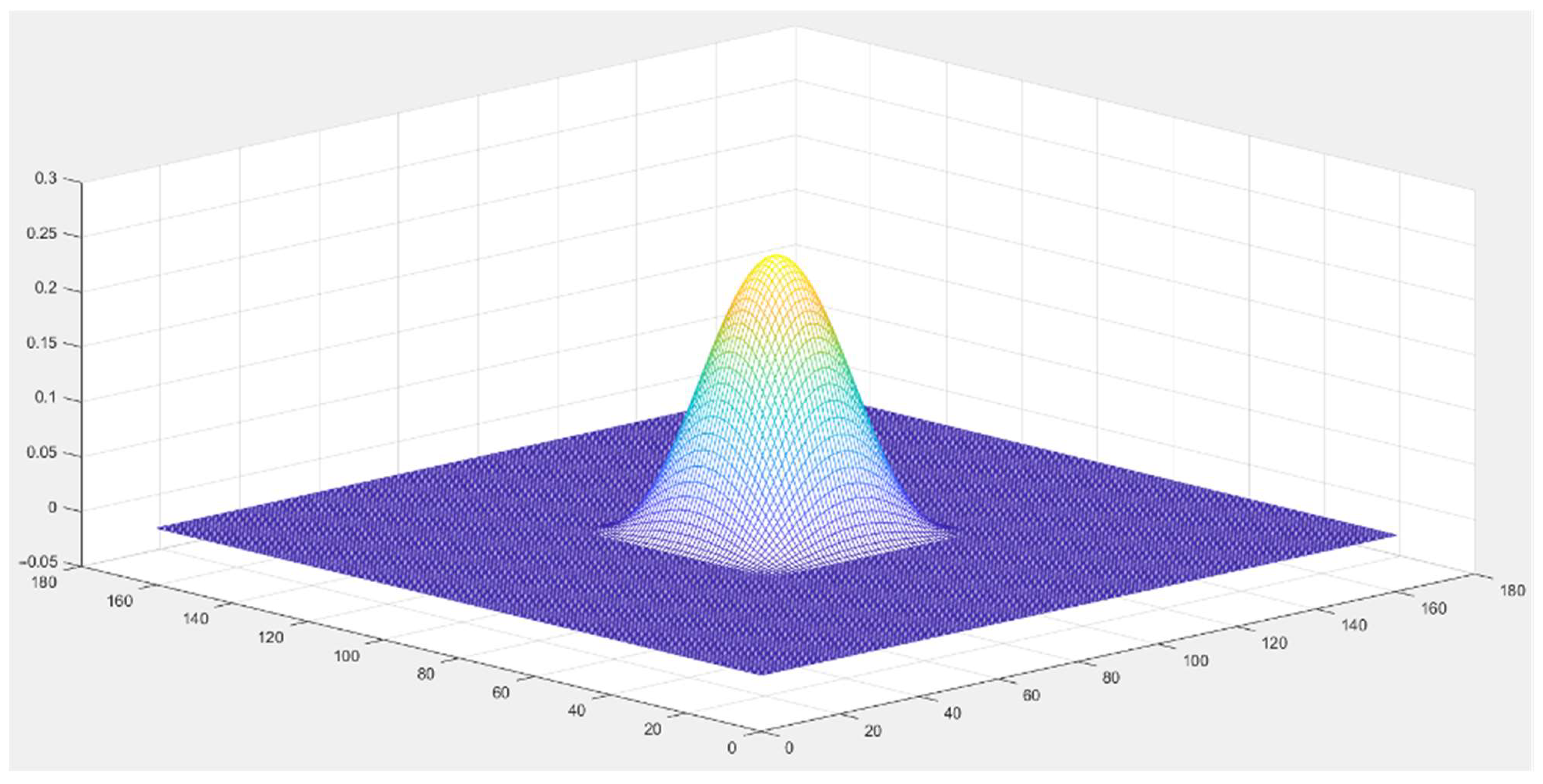
An example of solving problem (5) using the iterative extension method, when $a_1=1,$ is as follows:

$${\Omega }_1=(1;2)\times (1;2),\hspace{0.17em}\hspace{0.17em}{\Omega }_{{\rm I}{\rm I}}=(0;b)\times (0;b)\backslash [1;2]\times [1;2],\Pi =(0;b)\times (0;b),\hspace{0.17em}\hspace{0.17em}3<b\le 19/6,$$

and the boundaries of the regions have the following parts:

$$\begin{gathered} {\Gamma }_{1,0}=\left\{1,\hspace{0.17em}\hspace{0.17em}2\right\}\times (1;2)\cup (1;2)\times \left\{1,\hspace{0.17em}\hspace{0.17em}2\right\}, \\ {\Gamma }_{{\rm I}{\rm I},1}=\left\{b\right\}\times (0;b)\cup (0;b)\times \left\{b\right\},\hspace{0.17em}\hspace{0.17em}{\Gamma }_{{\rm I}{\rm I},2}=\left\{0\right\}\times (0;b)\cup (0;b)\times \left\{0\right\}, \\ {\Gamma }_{{\rm I}{\rm I},3}=\left\{1,\hspace{0.17em}\hspace{0.17em}2\right\}\times (1;2)\cup (1;2)\times \left\{1,\hspace{0.17em}\hspace{0.17em}2\right\}, \\ {\Gamma }_1=\left\{b\right\}\times (0;b)\cup (0;b)\times \left\{b\right\},\hspace{0.17em}\hspace{0.17em}{\Gamma }_2=\left\{0\right\}\times (0;b)\cup (0;b)\times \left\{0\right\}. \end{gathered}$$

In this square area and an encircling stripe, a grid with nodes is defined:

$$(x_i;y_j)=\left((i-1,5)h;(j-1,5)h\right),\hspace{0.17em}\hspace{0.17em}h=3/(n-2),n=3m+2,\hspace{0.17em}\hspace{0.17em}m\in \mathbb{N},\hspace{0.17em}\hspace{0.17em}m\ge 3,\hspace{0.17em}\hspace{0.17em}b=3+0,5h,\hspace{0.17em}\hspace{0.17em}i=1,2\dots ,n,\hspace{0.17em}\hspace{0.17em}j=1,2\dots ,n.$$

With the right side expressed as follows:

$$\begin{gathered} {\stackrel{⌣}{f}}_1=512(3{(x-1)}^2{(x-2)}^2+ \\ +(6x^2-18x+13)(6y^2-18y+13)+3{(y-1)}^2{(y-2)}^2)+64{(x-1)}^2{(x-2)}^2{(y-1)}^2{(y-2)}^2 \end{gathered}$$

The solution to the original problem has the following form:

$${\stackrel{⌣}{u}}_1=64{(x-1)}^2{(x-2)}^2{(y-1)}^2{(y-2)}^2.$$

When solving a problem on a computer, the estimate is given as ${\rm E}=0.001$. The graphs of the last approximation and the exact solution almost coincide (Figure 1).

3. Analysis of Shielded Harmonic System

Let us consider a screened harmonic system in the three-dimensional case in variational form:

$${\stackrel{⌣}{u}}_{\omega }\in {\stackrel{⌣}{H}}_{\omega }:\hspace{0.17em}\hspace{0.17em}{\mathrm{A}}_{\omega }({\stackrel{⌣}{u}}_{\omega },{\stackrel{⌣}{v}}_{\omega })=F_{\omega }({\stackrel{⌣}{v}}_{\omega })\hspace{0.17em}\hspace{0.17em}\forall {\stackrel{⌣}{v}}_{\omega }\in {\stackrel{⌣}{H}}_{\omega }, F_{\omega }\in {H^{\prime }}^{\omega }, \omega \in \left\{1,{\rm I}{\rm I}\right\}, {\Omega }_{\omega }\subset {ℝ}^3,$$

(9)

where the Sobolev functions space is

$${\stackrel{⌣}{H}}_{\omega }={\stackrel{⌣}{H}}_{\omega }({\Omega }_{\omega })=\left\{{\stackrel{⌣}{v}}_{\omega }\in W_2^1(\Omega ):\hspace{0.17em}\hspace{0.17em}{\left.{\stackrel{⌣}{v}}_{\omega }\right|}_{{\Gamma }_1}=0\right\}$$

on a flat bounded area ${\Omega }_{\omega }$ with a boundary given as

$$\hspace{0.17em}\mathsf{\partial }{\Omega }_{\omega }=\hspace{0.17em}{\overline{s}}_{\omega },\hspace{0.17em}\hspace{0.17em}{s}_{\omega }={\Gamma }_{\omega ,1}\cup {\Gamma }_{\omega ,2},\hspace{0.17em}\hspace{0.17em}{\Gamma }_{\omega ,i}\cap {\Gamma }_{\omega ,j}=\mathsf{\varnothing }, \mathrm{if} \hspace{0.17em}i\ne j,\hspace{0.33em}\hspace{0.33em}i,j=1,2,$$

and the scalar product is

$${\mathrm{A}}_{\omega }({\stackrel{⌣}{u}}_{\omega },{\stackrel{⌣}{v}}_{\omega })={\displaystyle \underset{{\Omega }_{\omega }}{\int }({\stackrel{⌣}{u}}_{\omega x}{\stackrel{⌣}{v}}_{\omega x}+{\stackrel{⌣}{u}}_{\omega y}{\stackrel{⌣}{v}}_{\omega y}+{\stackrel{⌣}{u}}_{\omega z}{\stackrel{⌣}{v}}_{\omega z}+{\kappa }_{\omega }{\stackrel{⌣}{u}}_{\omega }{\stackrel{⌣}{v}}_{\omega })d{\Omega }_{\omega }}.$$

When $\hspace{0.17em}\omega =\hspace{0.17em}1,\hspace{0.17em}\hspace{0.17em}{\kappa }_1\ge 0,\hspace{0.33em}{\Gamma }_{1,1}=\mathsf{\varnothing }$, a solvable problem of a screened harmonic system in the three-dimensional case is considered. When $\hspace{0.17em}\omega =\hspace{0.17em}{\rm I}{\rm I},\hspace{0.17em}\hspace{0.17em}{\kappa }_{{\rm I}{\rm I}}\ge 0$, a fictitious problem of a screened harmonic system in the three-dimensional case is considered.

The extended harmonic system is

$$\stackrel{⌣}{u}\in \stackrel{⌣}{V}:\hspace{0.17em}\hspace{0.17em}{\mathrm{A}}_1(\stackrel{⌣}{u},I_1\stackrel{⌣}{v})+{\mathrm{A}}_{{\rm I}{\rm I}}(\stackrel{⌣}{u},\stackrel{⌣}{v})=F_1(I_1\stackrel{⌣}{v})\hspace{0.17em}\hspace{0.17em}\forall \stackrel{⌣}{v}\in \stackrel{⌣}{V},$$

(10)

where the extended solution space of the extended problem considered is the Sobolev space

$$\stackrel{⌣}{V}=\stackrel{⌣}{V}(\Pi )=\left\{\stackrel{⌣}{v}\in W_2^1(\Pi ):\hspace{0.17em}\hspace{0.17em}{\left.\stackrel{⌣}{v}\right|}_{{\Gamma }_1}=0\right\},$$

and the regions are ${\Omega }_1,\hspace{0.33em}{\Omega }_{{\rm I}{\rm I}}$ such that ${\overline{\Omega }}_1\cup {\overline{\Omega }}_{{\rm I}{\rm I}}=\Pi$, ${\Omega }_1\cap {\Omega }_{{\rm I}{\rm I}}=\mathsf{\varnothing }$, and the boundary of a region $\Pi$ also consists of the closure of unions of open disjoint areas:

$$\hspace{0.17em}\mathsf{\partial }\Pi =\hspace{0.17em}\overline{s},\hspace{0.17em}\hspace{0.17em}s={\Gamma }_1\cup {\Gamma }_2,\hspace{0.17em}\hspace{0.17em}{\Gamma }_i\cap {\Gamma }_j=\mathsf{\varnothing },\hspace{0.17em}i\ne j,\hspace{0.33em}\hspace{0.33em}i,j=1,2,$$

and a non-empty intersection of boundaries of the first and second areas is the closure of the intersection of the corresponding parts of the boundaries of these areas:

$$\mathsf{\partial }{\Omega }_1\cap \mathsf{\partial }{\Omega }_{{\rm I}{\rm I}}=\overline{S}, S={\Gamma }_{1,1}\cap {\Gamma }_{{\rm I}{\rm I},2}=\mathsf{\varnothing }.$$

The extended solution space contains a subspace of solutions to the extended problem

$${\stackrel{⌣}{V}}_1={\stackrel{⌣}{V}}_1\left(\Pi \right)=\left\{{\stackrel{⌣}{v}}_1\in \stackrel{⌣}{V}:{\stackrel{⌣}{v}}_1{|}_{\Pi \backslash {\Omega }_1}=0\right\}.$$

The extended problem uses arbitrary projecting operators of the extended space onto the subspace of solutions to the extended problem:

$$I_1:{\stackrel{⌣}{V}}_1\mapsto {\stackrel{⌣}{V}}_1,\hspace{0.33em}{\stackrel{⌣}{V}}_1=im\hspace{0.17em}{I}_1,\hspace{0.33em}{I}_1=I_1^2.$$

The extended screened harmonic system in a three-dimensional case is considered on a finite-dimensional subspace of the Sobolev space. The discretization of the extended harmonic system is analyzed when

$$\begin{gathered} \Pi =\left(0;b_1\right)\times \left(0;b_2\right)\times \left(0;b_3\right), \\ {\Gamma }_1=\left\{b_1\right\}\times \left(0;b_2\right)\times \left(0;b_3\right)\cup \left(0;b_1\right)\times \left\{b_2\right\}\times \left(0;b_3\right)\cup \left(0;b_1\right)\times \left(0;b_2\right)\times \left\{b_3\right\}, \\ {\Gamma }_2=\left\{0\right\}\times \left(0;b_2\right)\times \left(0;b_3\right)\cup \left(0;b_1\right)\times \left\{0\right\}\times \left(0;b_3\right)\cup \left(0;b_1\right)\times \left(0;b_2\right)\times \left\{0\right\}, \\ {b}_1,b_2,b_3\in \left(0;+\infty \right). \end{gathered}$$

A grid with nodes is defined in a rectangular area:

$$\begin{gathered} \left(x_i;y_j;z_p\right)=\left(\left(i-1.5\right)h_1;\left(j-1.5\right)h_2;\left(p-1.5\right)h_3\right), \\ {h}_1=b_1/\left(m-1.5\right), h_2=b_2/\left(n-1.5\right), h_3=b_3/\left(K-1.5\right), \\ i=1,2,\dots ,m,\hspace{0.33em}j=1,2,\dots ,n,\hspace{0.33em}p=1,2,\dots ,K,\hspace{0.33em}m-2,\hspace{0.33em}n-2,\hspace{0.33em}K-2\in \mathbb{N}. \end{gathered}$$

Grid functions are introduced:

$$\begin{gathered} v_{i,j,p}=v\left(x_i;y_j;z_p\right)\in ℝ,\hspace{0.33em}i=1,2,\dots ,m,\hspace{0.33em}j=1,2,\dots ,n,\hspace{0.33em}p=1,2,\dots ,K, \\ m-2,\hspace{0.33em}n-2,\hspace{0.33em}K-2\in \mathbb{N}. \end{gathered}$$

The completion of grid functions with linear basis functions is applied.

$$\begin{gathered} {\Phi }^{i,j,p}\left(x;y;z\right)={\Psi }^{1,i}\left(x\right){\Psi }^{2,j}\left(y\right){\Psi }^{3,p}\left(z\right), \\ i=2,\dots ,m,\hspace{0.33em}j=2,\dots ,n,\hspace{0.33em}p=2,\dots ,K,\hspace{0.33em}m-2,\hspace{0.33em}n-2,\hspace{0.33em}K-2\in \mathbb{N}, \\ {\Psi }^{1,i}\left(x\right)=\left[2/i\right]\Psi \left(x/h_1-i+3.5\right)+\Psi \left(x/h_1-i+2.5\right), \\ {\Psi }^{2,j}\left(y\right)=\left[2/j\right]\Psi \left(y/h_2-j+3.5\right)+\Psi \left(y/h_2-j+2.5\right), \\ {\Psi }^{3,p}\left(z\right)=\left[2/p\right]\Psi \left(z/h_3-p+3.5\right)+\Psi \left(z/h_3-p+2.5\right), \\ \Psi \left(z\right)=\left\{\begin{array}{c}z,\hspace{1em}z\in \left[0;1\right],\\ 2-z,\hspace{1em}z\in \left[1;2\right],\\ 0,\hspace{1em}z\in \left(0;2\right).\end{array}\right. \end{gathered}$$

The basis functions outside the rectangular region are considered to be zero:

$$\begin{gathered} {\Phi }^{i,j,p}\left(x;y;z\right)=0,\hspace{0.33em}\left(x;y;z\right)\notin \Pi , \\ i=2,\dots ,m,\hspace{0.33em}j=2,\dots ,n,\hspace{0.33em}p=2,\dots ,K,\hspace{0.33em}m-2,\hspace{0.33em}n-2,\hspace{0.33em}K-2\in \mathbb{N}. \end{gathered}$$

Linear combinations of basis functions define a finite-dimensional subspace in the extended solution space.

$$\tilde{V}=\left\{\tilde{v}={\displaystyle \sum _{i=2}^{m-1}{\displaystyle \sum _{j=2}^{n-1}{\displaystyle \sum _{p=2}^{K-1}{v}_{i,j,p}{\Phi }^{i,j,p}\left(x;y;z\right)}}}\right\}\subset \stackrel{⌣}{V}.$$

The extended system is considered in Euclidean space. The approximated extended system problem is considered in matrix form as a system of linear algebraic equations. We approximate the problem for an extended system using a finite-dimensional subspace and obtain a system of equations.

$$\overline{u}\in {ℝ}^N:B\overline{u}=\overline{f},\hspace{0.33em}\overline{f}\in {ℝ}^N.$$

(11)

Let us consider that the projection operator onto the solution space of the extended problem nullifies the coefficients of basis functions whose supports are not completely contained in the first domain. We obtain the extended system problem in matrix form if we define the extended matrix and the extended right-hand side of the system as follows:

$$\begin{gathered} 〈B\overline{u},\overline{v}〉=A_1\left(\tilde{u},I_1\tilde{v}\right)+A_{{\rm I}{\rm I}}\left(\tilde{u},\tilde{v}\right)\hspace{0.33em}\forall \tilde{u},\tilde{v}\in \tilde{V},\hspace{0.33em}〈\overline{f},\overline{v}〉=F_1\left(I_1\tilde{v}\right)\hspace{0.33em}\forall \tilde{v}\in \tilde{V}, \\ \hspace{0.33em}〈\overline{f},\overline{v}〉=\left(\overline{f},\overline{v}\right)h_1{h}_2{h}_3=\overline{f}\overline{v}{h}_1{h}_2{h}_3, \\ \overline{v}=\left(v_1,v_2,\dots ,v_N\right)’\in {ℝ}^N,\hspace{0.33em}N=\left(m-2\right)\left(n-2\right)\left(K-2\right). \end{gathered}$$

In this case, the basis functions whose supports lie entirely in the first region are enumerated first. Then, the basis functions whose supports intersect the boundary of the first region and the second region together are enumerated. Finally, the basis functions whose supports lie entirely in the second region are enumerated. With this numbering, the resulting vectors have the following form:

$$\overline{v}=\left({\overline{v}}_1^{\prime },{\overline{v}}_2^{\prime },{\overline{v}}_3^{\prime }\right)\prime ,\hspace{0.33em}\hspace{0.33em}\overline{u}=\left({\overline{u}}_1^{\prime },{\overline{0}}^{\prime },{\overline{0}}^{\prime }\right)\prime ,\hspace{0.33em}\hspace{0.33em}\overline{f}=\left({\overline{f}}_1^{\prime },{\overline{0}}^{\prime },{\overline{0}}^{\prime }\right)\prime .$$

The matrix has a well-known structure:

$$B=\left[\begin{array}{ccc}{A}_{11}& A_{12}& 0\\ 0& A_{02}& A_{23}\\ 0& A_{32}& A_{33}\end{array}\right].$$

The extended problem is solved in matrix form:

$$B\overline{u}=\overline{f},\hspace{0.33em}\left[\begin{array}{ccc}{A}_{11}& A_{12}& 0\\ 0& A_{02}& A_{23}\\ 0& A_{32}& A_{33}\end{array}\right]\left[\begin{array}{c}\overline{u_1}\\ \overline{0}\\ \overline{0}\end{array}\right]=\left[\begin{array}{c}\overline{f_1}\\ \overline{0}\\ \overline{0}\end{array}\right].$$

The solution to the original problem in matrix form and the zero solution to the fictitious problem in matrix form are

$$A_{11}\overline{u_1}={\overline{f}}_1,\hspace{0.33em}\left[\begin{array}{cc}{A}_{02}& A_{23}\\ A_{32}& A_{33}\end{array}\right]\left[\begin{array}{c}\overline{u_2}\\ \overline{u_3}\end{array}\right]=\left[\begin{array}{c}\overline{0}\\ \overline{0}\end{array}\right],\hspace{0.33em}\left[\begin{array}{c}\overline{u_2}\\ \overline{u_3}\end{array}\right]=\left[\begin{array}{c}\overline{0}\\ \overline{0}\end{array}\right].$$

The matrices generated by scalar products are defined as

$$〈A_1\overline{u},\overline{v}〉=A_1\left(\tilde{u},\tilde{v}\right),\hspace{0.33em}〈A_{{\rm I}{\rm I}}\overline{u},\overline{v}〉=A_{{\rm I}{\rm I}}\left(\tilde{u},\tilde{v}\right)\hspace{0.33em}\forall \tilde{u},\tilde{v}\in \tilde{V}.$$

These matrices have the following structure:

$$A_{{\rm I}}=\left[\begin{array}{ccc}{A}_{11}& A_{12}& 0\\ A_{21}& A_{20}& 0\\ 0& 0& 0\end{array}\right],A_{{\rm I}{\rm I}}=\left[\begin{array}{ccc}0& 0& 0\\ 0& A_{02}& A_{23}\\ 0& A_{32}& A_{33}\end{array}\right].$$

A subspace of vectors is introduced:

$$\overline{V_1}=\left\{\overline{v}={\left({{\overline{v}}_1}^{\prime },{{\overline{v}}_2}^{\prime },{{\overline{v}}_3}^{\prime }\right)}^{\prime }\in {ℝ}^N:{\overline{v}}_2=\overline{0,}\hspace{0.33em}{\overline{v}}_3=\overline{0}\right\}.$$

Additionally, a subspace of vectors is defined:

$$\overline{V_2}=\left\{\overline{v}={\left({{\overline{v}}_1}^{\prime },{{\overline{v}}_2}^{\prime },{{\overline{v}}_3}^{\prime }\right)}^{\prime }\in {ℝ}^N:A_{11}{\overline{v}}_1+A_{12}{\overline{v}}_2=\overline{0,}\hspace{0.33em}{A}_{32}{\overline{v}}_2+A_{33}{\overline{v}}_3=\overline{0}\right\}.$$

An asymptotically optimal analysis of the extended system is performed based on the method of iterative extensions [13,14]. To solve problem (11), a method of iterative extensions is applied. The extended matrix is defined as the sum of the first matrix and the second matrix, multiplied by a positive parameter.

$$\begin{gathered} C=A_{{\rm I}}+\gamma A_{{\rm I}{\rm I}}, \\ \left[\begin{array}{ccc}{C}_{11}& C_{12}& 0\\ C_{21}& C_{22}& C_{23}\\ 0& C_{32}& C_{33}\end{array}\right]=\left[\begin{array}{ccc}{A}_{11}& A_{12}& 0\\ A_{21}& A_{20}& 0\\ 0& 0& 0\end{array}\right]+\gamma \left[\begin{array}{ccc}0& 0& 0\\ 0& A_{02}& A_{23}\\ 0& A_{32}& A_{33}\end{array}\right], \gamma \in \left(0;+\infty \right). \end{gathered}$$

It is assumed that the continuation provisions comply with the following:

$$\begin{gathered} \exists {\gamma }_1\in \left(0;+\infty \right),{\gamma }_2\in \left[{\gamma }_1;+\infty \right):{\gamma }_1^2〈C{\overline{v}}_2,C{\overline{v}}_2〉\le 〈A_{{\rm I}{\rm I}}{\overline{v}}_2,A_{{\rm I}{\rm I}}{\overline{v}}_2〉\le {\gamma }_2^2〈C{\overline{v}}_2,C{\overline{v}}_2〉\hspace{0.33em}\forall {\overline{v}}_2\in {\overline{V}}_2, \\ \exists \alpha \in \left[0;+\infty \right):〈A_{{\rm I}}{\overline{v}}_2,A_{{\rm I}}{\overline{v}}_2〉\le {\alpha }^2〈A_{{\rm I}{\rm I}}{\overline{v}}_2,A_{{\rm I}{\rm I}}{\overline{v}}_2〉\hspace{0.33em}\forall {\overline{v}}_2\in {\overline{V}}_2. \end{gathered}$$

The method of iterative extensions is a generalization of the fictitious domain method [12], where additional parameters are used when choosing extended matrices, and the iterative parameters are selected with the method of minimal residuals [15].

$${\overline{u}}^k\in {ℝ}^N:C({\overline{u}}^k-{\overline{u}}^{k-1})=-{\tau }_{k-1}(B{\overline{u}}^{k-1}-\overline{f}), k\in \mathbb{N},$$

(12)

$$\forall {\overline{u}}^0\in {\overline{V}}_1, \gamma >\alpha , {\tau }_0=1, {\tau }_{k-1}=〈{\overline{r}}^{k-1},{\overline{\eta }}^{k-1}〉/〈{\overline{\eta }}^{k-1},{\overline{\eta }}^{k-1}〉, k\in \mathbb{N}\backslash \left\{1\right\},$$

where, to calculate the iterative parameters, residuals, corrections, and equivalent residuals are sequentially calculated.

$${\overline{r}}^{k-1}=B{\overline{u}}^{k-1}-\overline{f}, {\overline{w}}^{k-1}=C^{-1}{\overline{r}}^{k-1}, {\overline{\eta }}^{k-1}=B{\overline{w}}^{k-1}, k\in \mathbb{N}.$$

The norm generated by the extended matrix is

$${‖\overline{v}‖}_{C^2}=\sqrt{〈C^2\overline{v},\overline{v}〉}\hspace{0.33em}\forall \overline{v}\in {ℝ}^N.$$

Theorem 2. 

For the method of iterative extensions (12) when analyzing a screened harmonic system in the three-dimensional case, the convergence is estimated as

$${‖{\overline{u}}^k-\overline{u}‖}_{C^2}\le \epsilon {‖{\overline{u}}^0-\overline{u}‖}_{C^2},\epsilon =2\left({\gamma }_2/{\gamma }_1\right){\left(\alpha /\gamma \right)}^{k-1},k\in \mathbb{N}.$$

An algorithm for solving the problem of and extended system in Euclidean space is given. When choosing iterative parameters, the method of minimal residuals is used.

I. Start with the zero initial approximation.

$$\forall {\overline{u}}^0\in {\overline{V}}_1, {\tau }_0=1.$$

II. Calculate the residual.

$${\overline{r}}^{k-1}=B{\overline{u}}^{k-1}-\overline{f}, k\in \mathbb{N}.$$

III. Calculate the value of the squared norm of the initial absolute error, which is preserved throughout all calculations.

$${{\rm E}}_{k-1}=〈{\overline{r}}^{k-1},{\overline{r}}^{k-1}〉, k\in \mathbb{N}.$$

IV. Calculate the correction.

$${\overline{w}}^{k-1}:C{\overline{w}}^{k-1}={\overline{r}}^{k-1}$$

V. Calculate the equivalent residual.

$${\overline{\eta }}^{k-1}=B{\overline{w}}^{k-1}, k\in \mathbb{N}\backslash \left\{1\right\}.$$

VI. Calculate the optimal value of the iterative parameter.

$${\tau }_{k-1}=〈{\overline{r}}^{k-1},{\overline{\eta }}^{k-1}〉/〈{\overline{\eta }}^{k-1},{\overline{\eta }}^{k-1}〉, k\in \mathbb{N}\backslash \left\{1\right\}.$$

VII. Find the new approximation.

$${\overline{u}}^k={\overline{u}}^{k-1}-{\tau }_{k-1}{\overline{w}}^{k-1}, k\in \mathbb{N}.$$

VIII. Check the iteration stop criterion for a given estimation of the relative error.

$${{\rm E}}_{k-1}\le {{\rm E}}^2{{\rm E}}_0, k\in \mathbb{N}\backslash \left\{1\right\}, E\in \left(0;1\right).$$

An example of solving problem (9) with the method of iterative extensions is given in the following domains:

$$\begin{gathered} {\Omega }_1=(0;2.5)\times (0;2.5)\times (0;2.5)\backslash [1.5;2.5)\times [1.5;2.5)\times [1.5;2.5), \\ {\Omega }_2=(1.5;2.5)\times (1.5;2.5)\times (1.5;2.5), \end{gathered}$$

with

$$\begin{gathered} {\stackrel{⌣}{f}}_1=((392-384x)(64y^3-196y^2+225)(64z^3-196z^2+225)+ \\ +(64x^3-196x^2+225)(392-384y)(64z^3-196z^2+225)+ \\ +(64x^3-196x^2+225)(64y^3-196y^2+225)(392-384z))/{225}^3, \\ {\stackrel{⌣}{u}}_1=(64x^3-196x^2+225)(64y^3-196y^2+225)(64z^3-196z^2+225)/{225}^3. \end{gathered}$$

The projected last approximation to the solution is displayed in Figure 1 with the specified $n=54,$ and the evaluation criterion ${\rm E}=0.001$. The red grid represents projected solution ${\stackrel{⌣}{u}}_1,$ and the blue surface represents the projected last approximation (Figure 2).

4. Conclusions

A new method of iterative extensions is developed, which is asymptotically optimal in terms of the number of operations, with automation for the optimal selection of iterative parameter values during information processing. This method is designed for the analysis of the shielded harmonic system in a three-dimensional case and the shielded biharmonic system.

The method of iterative extensions for shielded biharmonic systems and shielded harmonic systems in the three-dimensional case is implemented in the form of an iterative algorithm with a stop criterion when a predetermined and required accuracy is achieved.

The problems under consideration are linear and stationary, but the methods for solving them are nonlinear and nonstationary. This may be related to the study of single wave solutions using an improved algebraic method for the new extended Sakovich equations in fluid dynamics [16].

The developed method and algorithm of iterative extensions allow for generalizations for the analysis of a wide range of other systems that describe various stationary physical systems.

References

1. Bank, R.E.; Rose, D.J. Marching algorithms for elliptic boundary value problems. SIAM J. Numer. Anal. 1977, 14, 792–829. [Google Scholar] [CrossRef]
2. Ushakov, A.; Zagrebina, S.; Aliukov, S.; Alabugin, A.; Osintsev, K. A Review of Mathematical Models of Elasticity Theory Based on the Methods of Iterative Factorizations and Fictitious Components. Mathematics 2023, 11, 420. [Google Scholar] [CrossRef]
3. Ushakov, A.L. Research of the boundary value problem for the Sophie Germain Equations in a cyber-physical system. In Studies in Systems, Decision and Control; Springer: Berlin/Heidelberg, Germany, 2021; Volume 338, pp. 51–63. [Google Scholar]
4. Aubin, J.P. Approximate Solution of Elliptic Boundary Value Problems; Mir: Moscow, Russia, 1977; 383p. [Google Scholar]
5. Oganesyan, L.A.; Rukhovetz, L.A. Variational Difference Methods of Solving Elliptic Equations; AN ArmSSR: Yerevan, Armenia, 1979. [Google Scholar]
6. Landau, L.D. Elasticity Theory; Nauka: Moscow, Russia, 1965. [Google Scholar]
7. Dyakonov, E.G. Minimizing computational work. In Asymptotically Optimal Algorithms for Elliptic Problems; Nauka: Moscow, Russia, 1989; 272p. [Google Scholar]
8. Matsokin, A.M.; Nepomnyashchikh, S.V. Fictitious space method and explicit continuation operators. J. Comput. Math. Math. Phys. 1993, 33, 52–68. [Google Scholar]
9. Sorokin, S.B. Reconditioning in the numerical solution of the Dirichlet problem for a biharmonic equation. Sib. J. Comput. Math. 2011, 14, 205–213. [Google Scholar]
10. Sorokin, S.B. Analytical solution of a generalized spectral problem in the method of recalculating boundary conditions for a biharmonic equation. Sib. J. Comput. Math. 2013, 16, 267–274. [Google Scholar] [CrossRef]
11. Sorokin, S.B. Exact constants of energy equivalence in the method of recalculating boundary conditions for the biharmonic equation. Bull. Novosib. State Univ. Ser. Math. Mech. Comput. Sci. 2013, 13, 113–121. [Google Scholar]
12. Marchuk, G.I.; Kuznetsov, Y.A.; Matsokin, A.M. Fictitiois Domain and Domain Decomposition Methods. Russ. J. Numer. Anal. Math. Model. 1986, 1, 3–35. [Google Scholar] [CrossRef]
13. Ushakov, A.L.; Meltsaykin, E.A. Analysis of Biharmonic and Harmonic Models by the Methods of iterative Extensions. Bull. South Ural. State Univ. Ser. Math. Model. Program. Comput. Softw. 2022, 15, 51–66. [Google Scholar] [CrossRef]
14. Eremchuk, M.P.; Ushakov, A.L. Method of iterative Extensions for Analysis of a screened Harmonic systems. J. Comput. Eng. Math. 2023, 10, 3–16. [Google Scholar]
15. Samarsky, A.A.; Nikolaev, E.S. Methods for Solving Grid Functions; Science: Moscow, Russia, 1978. [Google Scholar]
16. Sakovich, S. A new Painlevé-integrable equation possessing KdV-Type solitons. Nonlinear Phenom Complex Syst. 2019, 22, 299–304. [Google Scholar]
Figure 1. Graphs of the exact solution and iterative solution.
Mathematics 12 00918 g001
Figure 2. Projected solution and projected last approximation.
Mathematics 12 00918 g002
Disclaimer/Publisher’s Note: The statements, opinions and data contained in all publications are solely those of the individual author(s) and contributor(s) and not of MDPI and/or the editor(s). MDPI and/or the editor(s) disclaim responsibility for any injury to people or property resulting from any ideas, methods, instructions or products referred to in the content.