Abstract
This paper discusses the approximate distributions of eigenvalues of a singular Wishart matrix. We give the approximate joint density of eigenvalues by Laplace approximation for the hypergeometric functions of matrix arguments. Furthermore, we show that the distribution of each eigenvalue can be approximated by the chi-square distribution with varying degrees of freedom when the population eigenvalues are infinitely dispersed. The derived result is applied to testing the equality of eigenvalues in two populations.
MSC:
62E15; 62H10
1. Introduction
The Wishart matrix is a symmetric random matrix defined by the sum of squares and cross-products of samples from a multivariate normal distribution. It becomes non-singular when the dimension is smaller than or equal to the number of observations; otherwise, it is singular. The distributions for the Wishart matrix and its eigenvalues have been used in many areas of science and technology, including multivariate analysis, Bayesian statistics, random matrix theory, and wireless communications. Some exact distributions of eigenvalues for a Wishart matrix are represented by the hypergeometric functions of matrix arguments. James [1] classified multivariate statistics problems into five categories based on hypergeometric functions. However, the convergence of these functions is slow, and their numerical computation is cumbersome when sample sizes or dimensions are large. Consequently, the derivation of approximate distributions of eigenvalues has received a great deal of attention. Sugiyama [2] derived the approximate distribution for the largest eigenvalue through the integral representation of the confluent hypergeometric function. Sugiura [3] showed that the asymptotic distribution of the individual eigenvalues is expressed by a normal distribution for a large sample size. The chi-square approximation was discussed when the population eigenvalues are infinitely dispersed in Kato and Hashiguchi [4] and Takemura and Sheena [5]. Approximations for hypergeometric functions have been developed and applied to the multivariate distribution theory in Butler and Wood [6,7,8]. Butler and Wood [6] provided the Laplace approximation for the hypergeometric functions of a single matrix argument. The numerical accuracies for that approximation were shown in the computation of noncentral moments of Wilk’s lambda statistic and the likelihood ratio statistic for testing block independence. This approximation was extended to the case of two matrix arguments in Butler and Wood [7]. All the results addressed above were carried out for eigenvalue distributions for a non-singular Wishart matrix.
Recently, the distribution of eigenvalues for the non-singular case has been extended to the singular case; see Shimizu and Hashiguchi [9] and Shinozaki et al. [10]. Shimizu and Hashiguchi [9] showed the exact distribution of the largest eigenvalue for a singular case is represented in terms of the confluent hypergeometric function as well as the non-singular case. The generalized representation for the non-singular and singular cases under the elliptical model was provided by Shinozaki et al. [10].
This paper is organized as follows. In Section 2, we apply the Laplace approximation introduced by Butler and Wood [7] to the joint density of eigenvalues of a singular Wishart matrix. Furthermore, we show that the approximation for the distribution of the individual eigenvalues can be expressed by the chi-square distribution with varying degrees of freedom when the population covariance matrix has spiked eigenvalues. Section 3 discusses the equality of the individual eigenvalues in two populations. Finally, we evaluate the precision of the chi-square approximation by comparing it to the empirical distribution through Monte Carlo simulation in Section 4.
2. Approximate Distributions of Eigenvalues of a Singular Wishart Matrix
Suppose that an real Gaussian random matrix X is distributed as , where O is the zero matrix, is a positive symmetric matrix, and ⊗ is the Kronecker product. This means that the column vectors of X are independently and identically distributed (i.i.d.) from with sample size n, where 0 is the m-dimensional zero vector. The eigenvalues of are denoted by , and . Subsequently, we define the singular Wishart matrix as , where and its distribution is denoted by . The spectral decomposition of W is represented as , where with , and the matrix is satisfied by . The set of all matrices with orthonormal columns is called the Stiefel manifold, denoted by , where . The volume of is represented by
For the definition of the above exterior product , see page 63 of Muirhead [11]. If , Stiefel manifold coincides with the orthogonal groups . Uhlig [12] gave the density of W as
where and . Srivastava [13] represented the joint density of eigenvalues of W in a form that includes an integral over the Stiefel manifold;
where and .
The above integral over the Stiefel manifold was evaluated by Shimizu and Hashiguchi [9] as the hypergeometric functions of the matrix arguments. We approximate (1) by Laplace approximation for the hypergeometric functions of two matrix arguments provided by Butler and Wood [7].
For a positive integer k, let denote a partition of k with and . The set of all partitions with less than or equal to m is denoted by . The Pochhammer symbol for a partition is defined as , where and . For integers, and real symmetric matrices A and B, we define the hypergeometric function of two matrix arguments as
where , and is the zonal polynomial indexed by with the symmetric matrix A; see the details provided in Chapter 7 of Muirhead [11]. The hypergeometric functions with a single matrix are defined as
The special cases and of (3) are called the confluent and Gauss hypergeometric functions, respectively. Butler and Wood [6]. proposed a Laplace approximation of and through their integral expressions. They showed that the accuracy of that approximation is greater than the previous results. This approximation was extended to the complex case in Butler and Wood [8]. The important property of (2) is the integral representation over the orthogonal group.
where is the invariant measure on the orthogonal group . Integral representations (4) are a useful tool for obtaining an approximation of . Asymptotic expansions of are given in Anderson [14] when both two positive definite matrix arguments are widely spaced. Constantine and Muirhead [15] gave the asymptotic behavior of when the population eigenvalues are multiple. From the integral expression (4), Butler and Wood [7] provided Laplace approximations for .
Lemma 1.
Let the two diagonal matrices be and , where , , and have multiplicity , in which . Let . Then the Laplace approximation of is given as
where and Hessian J is defined in Butler and Wood [7].
Shimizu and Hashiguchi [9] showed the following relationship
for an matrix , where is an symmetric matrix and O is the zero matrix. From (5), the joint density (1) can be rewritten by
where is the matrix and the symbol “∝” means that a constant required for scaling is removed. Applying Laplace’s method to the above joint density, we have an approximation for the joint density of eigenvalues.
Proposition 1.
The joint density of eigenvalues of a singular Wishart matrix by Laplace approximation is expressed by
where .
Proof.
In order to derive the approximate distributions of individual eigenvalues, we define the spiked covariance model that implies the first k-th eigenvalues of are infinitely dispersed, namely
where . Under the condition of (9) when , Takemura and Sheena [5] proved that the distribution of individual eigenvalues for a non-singular Wishart matrix is approximated by a chi-square distribution. The improvement for that approximation, that is, when the condition listed in (9) cannot be assumed, was discussed in Tsukada and Sugiyama [16]. The following lemma was provided by Nasuda et al. [17] and Takemura and Sheena [5] in the non-singular case and could be easily extended to the singular case.
Lemma 2.
Let , where and be the eigenvalues of W. If , we have
in the sense that , ,
where .
From Proposition 1 and Lemma 2, we obtain the chi-square approximation that is the main result of this paper.
Theorem 1.
Let , where and be the eigenvalues of W. If , it holds that
where is a chi-square distribution with degrees of freedom and the symbol “” means convergence in the distribution.
Proof.
Corollary 1 shows the chi-square approximation when all population eigenvalues are infinitely dispersed.
Corollary 1.
Let , where and are the eigenvalues of W. If , it holds that
Proof.
The proof is provided in the Appendix A. □
In the context of the High Dimension-Low Sample Size (HDLSS) setting, the asymptotic behavior of the eigenvalue distribution of a sample covariance matrix was discussed in Ahn et al. [18], Bolivar-Cime and Perez-Abreu [19], Jung and Marron [20]. Jung and Marron [20] showed that the spiked sample eigenvalues are approximated by the chi-square distribution with a degree of freedom of n. In contrast, Theorem 1 provides the approximation of the distribution of individual eigenvalues by a chi-square distribution with varying degrees of freedom.
3. Application to Test for Equality of the Individual Eigenvalues
This section discusses testing for equality of individual eigenvalues of the covariance matrix in two populations. For testing problems, we give the approximate distribution of the statistic based on the derived results from the previous section.
Let an Gaussian random matrix be distributed as , where and . The eigenvalues of are denoted by , where . We denote the eigenvalues of by , where . For fixed j, we consider the test of the equality of the individual eigenvalues in two populations as
Sugiyama and Ushizawa [21] reduced (11) to the equality of variance test for the principal components and proposed a testing procedure using the Ansari-Bradley test. Takeda [22] proposed the test statistic with for (11) and derived the exact distribution of . Since Johnstone [23] indicated that the first few eigenvalues are very large compared to the others in the large dimensional setting, it is essential to understand how the distribution for the first few eigenvalues is constructed. We provide the exact density function of with in the same way as Takeda [22].
Theorem 2.
Let and be two independent Wishart matrices with distribution and , respectively, where . Then we have the density of as
where , and
Proof.
As the dimension increases, it is difficult to perform the numerical computation of (12) due to the high computational complexity. From Theorem 1, we provide the approximate distribution for (12) by F-distribution.
Corollary 2.
Let and be two independent Wishart matrices with distribution and , respectively, where and are the eigenvalues of . If the first k-th eigenvalues of are spiked, then we have
where F is an F distribution with and degrees of freedom.
4. Simulation Study
We investigate the accuracy of the approximation for the derived distributions. In the simulation study, we consider the following population covariance matrix:
where . In the large-dimensional setting, mainly the accuracy of the approximate distributions for the largest and second eigenvalues was investigated; see Iimori et al. [24]. In (15), we set as Case 1 and as Case 2. These two cases imply that the population covariance matrix has two spiked eigenvalues. Parameter in (9) is smaller in Case 1 than in Case 2. We denote and as the chi-square distributions with n and degrees of freedom, which are the approximate distributions of the largest and second eigenvalues, respectively. The empirical distribution based on Monte Carlo simulations is denoted by . Table 1 and Table 2 show the -percentile points of the distributions of and for and , respectively. From the simulation study, we know that sufficient accuracy of approximation for the largest eigenvalue has already been obtained in Case 2. Case 1 is more accurate than Case 2 for the second eigenvalue. It is seen that the desired accuracy can be achieved when the parameter is small.

Table 1.
Percentile points of the distributions of and of (Case 1).
Table 2.
Percentile points of the distributions of and of (Case 2).
Table 3 and Table 4 present the chi-square probabilities for Case 1 in 90% 95% 99% percentile points denoted as , , and from the empirical distribution. We denote and as the chi-square approximation of the distributions for the largest and second largest eigenvalues, respectively. In this simulation study, we set , and . It can be observed that all probabilities are close to the true theoretical probabilities.
Table 3.
Approximate probabilities of based on the empirical percentile points (Case 1).
Table 4.
Approximate probabilities of based on the empirical percentile points (Case 1).
Finally, we provide the graph of the density of F distribution in Corollary 2 compared to the empirical distribution function. In Figure 1, we superimpose the graph of the F approximation with the histogram of for and in Case 2. The vertical line and histograms show the empirical distribution of the based on iteration, respectively. The solid line is the density function of the F distribution. From the points of , we can confirm that the approximate probability is 0.950.
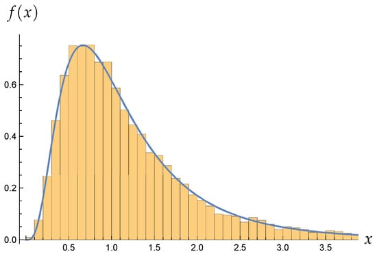
Figure 1.
and .
5. Concluding Remarks
In this study, we provided the approximate distribution of eigenvalues of the singular Wishart matrix, which is similar to the result of Takemura and Sheena [5] for the non-singular case. Through numerical experiments, we confirmed that the approximation accuracy is sufficient when the parameter is small. The distribution approximation proposed by Tsukada and Sugiyama [16] might be useful to improve the derived approximate results when is not assumed. As a part of future work, it would be desirable to examine the robustness of the chi-square approximation to normality assumption.
Author Contributions
Conceptualization, K.S.; methodology, K.S. and H.H.; software, K.S.; validation, H.H.; investigation, K.S. and H.H.; writing—original draft, K.S.; writing—review and editing, H.H. All authors have read and agreed to the published version of the manuscript.
Funding
This work was supported by JSPS KAKENHI Grant Numbers 23K19015 and 23K11016.
Data Availability Statement
No new data were created or analyzed in this study. Data sharing is not applicable to this article.
Conflicts of Interest
The authors declare no conflict of interest.
Correction Statement
This article has been republished with a minor correction to the Document Type. This change does not affect the scientific content of the article.
Appendix A
Proof of Corollary 1
References
- James, A.T. Distribution of matrix variates and latent roots derived from normal samples. Ann. Math. Stat. 1964, 35, 475–501. [Google Scholar] [CrossRef]
- Sugiyama, T. Approximation for the distribution of the largest latent root of a Wishart matrix. Aust. J. Stat. 1972, 14, 17–24. [Google Scholar] [CrossRef]
- Sugiura, N. Derivatives of the characteristic root of a symmetric or a hermitian matrix with two applications in multivariate analysis. Commun. Stat. Theory Methods 1973, 1, 393–417. [Google Scholar] [CrossRef]
- Kato, H.; Hashiguchi, H. Chi-square approximations for eigenvalue distributions and confidential interval construction on population eigenvalues. Bull. Comput. Stat. Jpn. 2014, 27, 11–28. [Google Scholar]
- Takemura, A.; Sheena, Y. Distribution of eigenvalues and eigenvectors of Wishart matrix when the population eigenvalues are infinitely dispersed and its application to minimax estimation of covariance matrix. J. Multivar. Anal. 2005, 94, 271–299. [Google Scholar] [CrossRef]
- Butler, R.W.; Wood, T.A. Laplace approximations for hypergeometric functions with matrix argument. Ann. Stat. 2002, 30, 1155–1177. [Google Scholar] [CrossRef]
- Butler, R.W.; Wood, T.A. Laplace approximations to hypergeometric functions of two matrix arguments. J. Multivar. Anal. 2005, 94, 1–18. [Google Scholar] [CrossRef]
- Butler, R.W.; Wood, T.A. Laplace approximations for hypergeometric functions with Hermitian matrix argument. J. Multivar. Anal. 2022, 192, 105087. [Google Scholar] [CrossRef]
- Shimizu, K.; Hashiguchi, H. Heterogeneous hypergeometric functions with two matrix arguments and the exact distribution of the largest eigenvalue of a singular beta-Wishart matrix. J. Multivar. Anal. 2021, 183, 104714. [Google Scholar] [CrossRef]
- Shinozaki, A.; Shimizu, K.; Hashiguchi, H. Generalized heterogeneous hypergeometric functions and the distribution of the largest eigenvalue of an elliptical Wishart matrix. Random Matrices Theory Appl. 2022, 11, 2250034. [Google Scholar] [CrossRef]
- Muirhead, R.J. Aspects of Multivariate Statistical Theory; Wiley: New York, NY, USA, 1982. [Google Scholar]
- Uhlig, H. On Singular Wishart and singular multivariate beta distributions. Ann. Stat. 1994, 22, 395–405. [Google Scholar] [CrossRef]
- Srivastava, M.S. Singular Wishart and multivariate beta distributions. Ann. Stat. 2003, 31, 1537–1560. [Google Scholar] [CrossRef]
- Anderson, G.A. An asymptotic expansion for the distribution of the latent roots of the estimated covariance matrix. Ann. Math. Stat. 1965, 36, 1153–1173. [Google Scholar] [CrossRef]
- Constantine, A.G.; Muirhead, R.T. Asymptotic expansions for distributions of latent roots in multivariate analysis. J. Multivar. Anal. 1976, 3, 369–391. [Google Scholar] [CrossRef]
- Tsukada, S.; Sugiyama, T. Distribution approximation of covariance matrix eigenvalues. Comm. Statist. Simul. Comput. 2023, 52, 4313–4325. [Google Scholar] [CrossRef]
- Nasuda, R.; Shimizu, K.; Hashiguchi, H. Asymptotic behavior of the distributions of eigenvalues for beta-Wishart ensemble under the dispersed population eigenvalues. Commun. Stat. Theory Methods 2023, 52, 7840–7860. [Google Scholar] [CrossRef]
- Ahn, J.; Marron, J.S.; Muller, K.M.; Chi, Y. The high-dimension, low-sample-size geometric representation holds under mild conditions. Biometrika 2007, 94, 760–766. [Google Scholar] [CrossRef]
- Bolivar-Cime, A.; Perez-Abreu, V. PCA and eigen-inference for a spiked covariance model with largest eigenvalues of same asymptotic order. Braz. J. Probab. Stat. 2014, 28, 255–274. [Google Scholar] [CrossRef]
- Jung, S.; Marron, J.S. PCA consistency in high dimension, low sample size context. Ann. Stat. 2009, 37, 4104–4130. [Google Scholar] [CrossRef]
- Sugiyama, T.; Ushizawa, K. A non-parametric method to test equality of intermediate latent roots of two populations in a principal component analysis. J. Jpn. Stat. Soc. 1998, 28, 227–235. [Google Scholar] [CrossRef][Green Version]
- Takeda, Y. Permutation test for equality of each characteristic root in two populations. J. Jpn. Soc. Comput. Stat. 2001, 14, 1–10. [Google Scholar] [CrossRef]
- Johnstone, I.M. On the distribution of the largest eigenvalue in principal components analysis. Ann. Stat. 2001, 29, 295–327. [Google Scholar] [CrossRef]
- Iimori, T.; Ogura, T.; Sugiyama, T. On the distribution of the second-largest latent root for certain high dimensional Wishart matrices. Int. J. Knowl. Eng. Soft Data Paradig. 2013, 4, 187–197. [Google Scholar] [CrossRef]

Disclaimer/Publisher’s Note: The statements, opinions and data contained in all publications are solely those of the individual author(s) and contributor(s) and not of MDPI and/or the editor(s). MDPI and/or the editor(s) disclaim responsibility for any injury to people or property resulting from any ideas, methods, instructions or products referred to in the content. |
© 2024 by the authors. Licensee MDPI, Basel, Switzerland. This article is an open access article distributed under the terms and conditions of the Creative Commons Attribution (CC BY) license (https://creativecommons.org/licenses/by/4.0/).