Article

Adaptive Fuzzy Backstepping Control for Itô-Type Nonlinear Switched Systems Subject to Unknown Hysteresis Input

Jinan Campus (Swinburne College), Shandong University of Science and Technology, Jinan 250031, China
*
Author to whom correspondence should be addressed.
Mathematics 2024, 12(7), 1070; https://doi.org/10.3390/math12071070
Submission received: 4 March 2024 / Revised: 31 March 2024 / Accepted: 31 March 2024 / Published: 2 April 2024

Abstract

:
The adaptive fuzzy backstepping control problem is studied for Itô-type nonlinear switched systems subject to unknown hysteresis input. Compared with existing works, the unknown hysteresis and stochastic disturbances are considered in the pure-feedback switched systems. The mean value theorem tackles the non-affine functions. The backstepping technique introduces an auxiliary virtual controller. In addition, the Nussbaum function is employed to solve the difficulty caused by the unknown hysteresis under arbitrary switching. Based on a fuzzy logic system and backstepping technique, a new adaptive control proposal is obtained, which ensures that the system states satisfy semiglobally uniformly ultimately bounded (SGUUB) in probability and that the tracking error converges to a region of the origin. Finally, we provide two examples to show the validity of the presented scheme.

1. Introduction and Related Work

1.1. Introduction

As hybrid systems, switched systems have received much attention recently [1,2,3,4,5,6,7,8,9,10,11,12,13,14,15,16,17]. A lot of outstanding results have been published; for instance, the switched system is widely applied in aircraft and air traffic systems [1], circuit and power systems [2], robot manipulator systems [3], and networked control systems [4]. It is widely known that the hysteresis phenomenon also often exists in many physical and engineering systems, such as networked control systems and circuit and power systems, e.g., [15,16].
In recent decades, nonlinear system control has received great concern from researchers due to its wide application; for instance, the optimization problem of prescribed performance tracking control was investigated for a class of strictly feedback nonlinear systems [18]; some new regressor-free adaptive controllers were proposed for cooperative robotic arms [19]. There always exist stochastic disturbances in practical physical plants [20]. The investigation of stochastic nonlinear systems has received considerable attention [21,22,23]. Among various kinds of stochastic nonlinear systems, one of the most important types is Itô stochastic nonlinear systems [24,25]. The backstepping design technique was first introduced for such systems [24]. Based on the results of [24], the output-feedback control problem was investigated [25]. Fuzzy control is a successful control approach for many complex nonlinear systems [26]. Fuzzy logic systems are commonly used in fuzzy control because they can approximate unknown nonlinear functions [27].
However, according to the authors, few results have been reported for stochastic nonlinear pure-feedback switched systems with stochastic disturbances and unknown hysteresis. More recently, the adaptive neural network control problem was investigated for stochastic pure-feedback switched systems with unknown hysteresis [28]. For nonlinear switched systems with unknown hysteresis, Liu et al. [29] proposed an adaptive finite-time tracking control scheme. However, these works only considered non-stochastic systems.
This paper provides an improved adaptive fuzzy control scheme based on the above observations. The developed control method is more general. The stochastic disturbances and unknown hysteresis are all considered for the pure-feedback switching systems. The non-affine functions are solved via the mean value theorem. An auxiliary virtual controller is introduced in the provided control scheme. The new properties of the Nussbaum function resolve the unknown direction hysteresis under the arbitrary switch. The novel adaptive fuzzy control scheme assures that system signals remain SGUUB in probability, and the tracking error converges to a region of the origin.
The others are arranged as below. Section 2 states the problem and preparations. In Section 3, an adaptive fuzzy tracking control is designed, and the main results are presented. Two examples are provided in Section 4. Finally, Section 5 summarizes the work.

1.2. Related Work

In this section, we first review the literature concerning switched systems and then the hysteresis nonlinearity problem.
For switched systems, researchers have widely investigated the stability analysis problem [5,6,7,8,9]. In [5], Yuan et al. presented the fuzzy adaptive tracking control for nonlinear systems via output feedback. Zhao et al. in [6] proposed a feasible control approach for nonlinear systems with unmeasured states. Two kinds of controllers are designed for nonlinear switched systems with unknown functions [7]. Recently, Xiong et al. [8] discussed the adaptive fuzzy fault-tolerant tracking problem by output feedback for a family of nonlinear switched systems with uncertainty. H filtering is considered for discrete-time linear switched systems in [9]. For nonlinear switched systems with uncertainty, the authors of [10] proposed an event-triggered adaptive fuzzy control scheme. For non-affine nonlinear systems with actuator faults, the authors of [11] considered an event-triggered adaptive fuzzy control problem. However, switched systems may have many complications due to the interaction between continuous and discrete dynamics [12,13]. Switching between subsystems could lead to instability [14]. Therefore, studies on stability for switched systems are more challenging than those for systems.
Due to the non-differentiability of hysteresis nonlinearity, the system performance is sometimes greatly aggravated and often shows undesired errors or vibrations, even leading to system instability [17,30]. In recent years, many results have been published for a series of hysteresis forms, for example, the Prandtl–Ishlinskii hysteresis model [31,32], Preisach model [33], Duhem hysteresis operator [34], backlash-like hysteresis (BLH) [35,36], and so on. Among them, the BLH model was widely used because it better represents the hysteresis nonlinearity and facilitates the control design. Recently, many notable results have been published [37,38,39,40,41,42]. Ref. [37] studied an adaptive fault-tolerant control design for a flexible Timoshenko arm with actuator failures, BLH, and external disturbances. Zhu et al. [38] designed the event-triggered controller for nonlinear systems with unknown BLH. In [39], an adaptive neural network control is proposed for an unknown two-degree-of-freedom helicopter system with unknown BLH and output constraints. The tracking control problem of nonlinear switched systems was solved with hysteresis input and arbitrary switching in finite-time intervals [40].
However, according to the authors, few results have been reported for stochastic nonlinear pure-feedback switched systems with stochastic disturbances and unknown hysteresis. To address this problem, we use a fuzzy logic system and backstepping technique and develop a new adaptive control proposal to ensure the system states satisfying SGUUB.

2. Problem Statement and Preliminaries

2.1. Problem Formulation

Consider the following equation:
d x = g ( x , t ) d t + f ( x , t ) d ω , x R n , t 0
where ω is 1-dimensional standard Brownian motion, which is defined on the complete probability space ( Ω , F , { F t } t 0 , P ) , where Ω is a sample space, F denotes a σ -field, { F t } t 0 is a filtration, and P represents a probability measure. x denotes the state, g and f satisfy locally Lipschitz conditions for x and g ( 0 , t ) = 0 , f ( 0 , t ) = 0 .
Definition 1 
([20]). A continuous function N ( ζ ) is called Nussbaum function, if it satisfies
lim s + s u p 1 s 0 s N ( ζ ) d ζ = + , lim s i n f 1 s 0 s N ( ζ ) d ζ = .
Definition 2. 
( I t o ^ formula) [21] For system (1) and any given V ( x , t ) C 2 , 1 , the following formula is called I t o ^ formula
L V = V t + V x g + 1 2 T r { f T 2 V x 2 f } ,
where L is the differential operator, T r ( A ) denotes the trace of matrix A R n × n , 1 2 T r { f T 2 V 2 x f } is an I t o ^ correction term.
Remark 1. 
In a later section, the I t o ^ formula is used to compute the differential of the Lyapunov function candidate. In I t o ^ correction term 1 2 T r { f T 2 V 2 x f } , the existence of the second-order differential 2 V 2 x makes the controller design much more difficult than that of the deterministic system.
Definition 3
(SGUUB) [41] The trajectory x ( t ) of system (1) is said to be SGUUB in pth moment, if for some compact set Ω R n and any initial state x 0 = x ( t 0 ) , there exist a constant ε > 0 , and a time constant T ˜ = T ˜ ( ε , x 0 ) such that E [ x ( t ) p ] < ε , for all t > t 0 + T ˜ , where E denotes the mathematic expectation operator. In particular, when p = 2 , it is usually called SGUUB in the mean square.
Lemma 1 
([22]). For system (1), if exist V ( x , t ) C 2 , 1 , smooth functions ϑ ( t ) and ξ ( x , t ) , Nussbaum even function N ( · ) satisfying
e c t V ( x , t ) ( η + M ( t ) ) e c t + 0 t ( ξ ( x , τ ) N ( ϑ ) ϑ ˙ + ϑ ˙ ) e c τ d τ ,
then V ( x , t ) , ϑ ( t ) and 0 t ( ξ ( x , τ ) N ( ϑ ) ϑ ˙ + ϑ ˙ ) d τ are bounded in probability, where 0 < ξ ( x , t ) l < , l , c are constants, η is a nonnegative stochastic variable, M ( t ) is a real valued continuous local martingale with M ( 0 ) = 0 .
Lemma 2 
([23]). For any θ ( t ) 0 , t t 0 , θ ^ ˙ ( t 0 ) 0 , then
θ ^ ˙ ( t ) = γ θ ^ ( t ) + κ ρ ( t ) ,
where constants γ , κ and function ρ ( t ) are positive.
Lemma 3 
([42]). (Young’s inequality). For x , y R , the following inequality holds,
x y ε s s | x | s + 1 h ε h | y | h ,
where ε > 0 , s > 1 , h > 1 , and ( s 1 ) ( h 1 ) = 1 .

2.2. Problem Formulation

In this section, the following switched system is considered
d x i = ( f i , σ ( t ) ( x ¯ i , x i + 1 ) + g i , σ ( t ) ( x ) ) d t + ψ i , σ ( t ) T ( x ¯ i ) d w , d x n = ( f n , σ ( t ) ( x ¯ n , u ) + g n , σ ( t ) ( x ) ) d t + ψ n , σ ( t ) T ( x ¯ n ) d w , y = x 1 , i Z n 1 = { 1 , 2 , , n 1 } ,
where x = [ x 1 , x 2 , , x n ] T R n and x ¯ i = [ x 1 , x 2 , , x i ] R i stand for the states, y R denotes the output, σ ( t ) is a continuous switching signal, where t [ 0 , ) , σ ( t ) M = { 1 , 2 , , m } . σ ( t ) = k ( k M ) indicates the k-th subsystem. w is explained in (1). f i , k ( · ) , g i , k ( · ) and ψ i , k ( · ) , i Z n are unknown smooth nonlinear functions. u ( t ) R is the input. An unknown Bouc–Wen hysteresis [43] satisfies
u ( t ) = H ( v ) = μ 1 v ( t ) + μ 2 ς ( t ) ,
where unknown hysteresis parameters μ 1 and μ 2 have the same symbol and the direction of hysteresis is controlled by μ 1 , for example, if μ 1 > 0 , then the direction of u ( t ) is positive. The input v ( t ) R and the auxiliary variable ς ( t ) satisfy
d ς = d v β | ς | n 1 ς | d v | χ | ς | n d v v ˙ f ( ς , v ˙ ) d t ,
where t [ 0 , ) , ς ( t 0 ) = 0 , parameters χ , n and β are unknown and satisfy n > 1 , β > | χ | . The shape and amplitude of u ( t ) are shown by χ , and the smoothness is determined by n for the transition from the initial slope to the slope of the asymptote. f ( ς , v ˙ ) = 1 s g n ( v ˙ ) β | ς | n 1 ς χ | ς | n , where ς in [43] satisfies
| ς | 1 β + χ n .
In the following, for system (4), an adaptive controller is designed, which ensures y tracks to a reference signal y d and all closed-loop system signals remain SGUUB in probability.
A continuous function f ( x ) , which is defined on a compact set Ω , is approximated by a fuzzy logic system (FLS). By singleton fuzzifier, center-average defuzzifier, and product inference methods, the fuzzy rules [44] are introduced as below:
R l : If x 1 is F 1 l … and x n is F n l , then y is G l , l Z N , where x = [ x 1 , x 2 , , x n ] T denotes the input of the fuzzy systems, y R is the output, F i l and G l are fuzzy sets, and N is the rule number. Meanwhile, the output of the fuzzy system is
y ( x ) = Σ l = 1 N Φ l Π i = 1 n μ F i l ( x i ) Σ l = 1 N [ Π i = 1 n μ F i l ( x i ) ] ,
where Φ l = max y R μ F i l ( x i ) , Φ = ( Φ 1 , Φ 2 , , Φ N ) T , the μ F i l ( x i ) , i Z n is the fuzzy membership function, which is constructed in the simulation example.
Remark 2. 
It is worth noting that μ F i l ( x i ) is usually chosen as the Gaussian basis function, which has clear physical significance such that the shape of each Gaussian function is determined by two parameters: the central point and the standard deviation. The central point and the standard deviation need to be determined. In general, the central points of membership functions are designed to be uniformly distributed over the universe of discourse by applying the trial-and-error approach. From the control performance point of view, a low standard deviation leads to the controller with high sensitivity; a high one leads to the controller with low sensitivity. Considering the practical application, the standard deviation is usually set as 2 in each membership function. Therefore, the membership function of x i is chosen as μ F i l ( x i ) = exp [ ( x i ϱ i l ) 2 π i l ] . where ϱ i l and π i l are the center and width.
Define the fuzzy basis function
ξ l ( x ) = Π i = 1 n μ F i l ( x i ) Σ l = 1 N [ Π i = 1 n μ F i l ( x i ) ] ,
and let
Y ( x ) = ( ξ 1 ( x ) , ξ 2 ( x ) , , ξ N ( x ) ) T .
Then y ( x ) is be reformulated as
y ( x ) = Φ T Y ( x ) .
Lemma 4 
([27]). Consider a continuous function f ( x ) , x Ω , for any ε > 0, there exists an FLS (7) such that
sup x Ω | f ( x ) Φ T Y ( x ) | ε ,
where weight vector Ω R N is a compact set, ε is fuzzy approximate error with ε 0 as l .
To facilitate the control design in Part 3, we give the following assumptions.
Assumption 1 
([23]). Let y ¯ d ( i ) = [ y d , y d ( 1 ) , y d ( 2 ) , , y d ( i ) ] T , i Z n , where y d ( i ) is the i- t h derivative of y d . y d and y d ( i ) are continuous and bounded. In addition, for system (4), let
h i , k ( x ¯ i , x i + 1 ) = f i , k ( x ¯ i , x i + 1 ) x i + 1 , x n + 1 = u , i Z n .
Assumption 2 
([23]). Given unknown constants b m and b M , the following holds
0 < b m | h i , k ( x ¯ i , x i + 1 ) | b M < ,
where x ¯ i R i , i Z n .
Remark 3. 
For i Z n 1 , the signs of { h i , k ( x ¯ i , x i + 1 ) } i Z n 1 are known; however, when i = n , h n , k ( x ¯ n , u ) is unknown.
For simplicity, without loss of generality, let h i , k ( x ¯ i , x i + 1 ) b m , where i Z n 1 . By the mean value theorem, one has
f i , k ( x ¯ i , x i + 1 ) f i , k ( x ¯ i , x i + 1 0 ) = h i , k ( x ¯ i , ξ i ) ( x i + 1 x i + 1 0 ) ,
where ( x 1 0 , x 2 0 , , x n 0 , v 0 ) T is an equilibrium point, let H ( v ) = u = x n + 1 , H ( v 0 ) = u 0 = x n + 1 0 , ξ i is a point between x i + 1 0 and x i + 1 . Based on the above, then (4) is rewritten as
d x i = ( f i , k ( x ¯ i , x i + 1 0 ) + h i , k ( x ¯ i , ξ i ) ( x i + 1 x i + 1 0 ) + g i , k ( x ) ) d t + ψ i , k T ( x ¯ i ) d w , d x n = ( f n , k ( x ¯ n , u 0 ) + h n , k ( x ¯ n , ξ n ) ( u u 0 ) + g n , k ( x ) ) d t + ψ n , k T ( x ¯ n ) d w , k M , y = x 1 , i = 1 , 2 , , n 1 .

3. Adaptive Fuzzy Tracking Control Design

In this part, an adaptive fuzzy control scheme is presented for (10) via a backstepping technique combined with a Nussbaum-type function. The backstepping procedure needs n steps, in which the coordinate transformation is needed at each step:
z 1 = x 1 y d , z i = x i α i 1 , i Z n ,
where α i 1 is an intermediate control function. To convenient the following design, define a constant θ i = max { Φ i , k b m } , where Φ i , k ( i Z n , k M ) is a FLS used to approximate an unknown function f i ¯ .
Remark 4. 
In the existing backstepping control schemes, all the elements need to be estimated online for weighting vectors. Given a n-th order nonlinear system, if N fuzzy sets for all the variables are used in the fuzzy controller, there are n N parameters to be estimated online. This implies that the online learning time becomes long. By estimating the Euclidean norm Φ i , k , the number of the adaptive parameters is reduced to n in this paper. Therefore, this algorithm can reduce the computation burden.
Step 1. Based on (11), the time derivative of z 1 is
d z 1 = ( f 1 , k ( x ¯ 1 , x 2 0 ) + h 1 , k ( x ¯ 1 , ξ 1 ) ( x 2 x 2 0 ) + g 1 ( x ) y ˙ d ) d t + ψ 1 , k T ( x ¯ 1 ) d w .
Define Lyapunov function
V 1 = 1 4 z 1 4 + b m 2 λ 1 θ ˜ 1 2 ,
where θ ˜ 1 = θ 1 θ ^ 1 denotes the parameter error, λ 1 is a positive designed constant (PDC). Combining (2) with (11) and (12), we can obtain
L V 1 = z 1 3 ( f 1 , k ( x 1 , x 2 0 ) + h 1 , k ( x ¯ 1 , ξ 1 ) ( z 2 + α 1 x 2 0 ) + g 1 ( x ) y ˙ d ) + 3 2 z 1 2 ψ 1 , k T ψ 1 , k b m λ 1 θ ˜ 1 θ ^ ˙ 1 .
According to Lemma 3 and (9), it is obtained easily
3 2 z 1 2 ψ 1 , k T ψ 1 , k 3 4 r 1 2 z 1 4 ψ 1 , k 4 + 3 4 r 1 2 ,
h 1 , k ( x ¯ 1 , ξ 1 ) z 1 3 z 2 3 4 b M z 1 4 + b M 4 z 2 4 ,
where r 1 is a PDC. We substitute (15) and (16) into (14), then
L V 1 z 1 3 ( f 1 , k ( x 1 , x 2 0 ) + 3 4 b M z 1 + h 1 , k ( x ¯ 1 , ξ 1 ) ( α 1 x 2 0 ) ) + g 1 ( x ) y ˙ d + 3 4 r 1 2 z 1 ψ 1 , k 4 ) + b M 4 z 2 4 + 3 4 r 1 2 b m λ 1 θ ˜ 1 θ ^ ˙ 1 .
Let f ¯ 1 , k = f 1 , k + 3 4 b M z 1 + g 1 ( x ) y ˙ d + 3 4 r 1 2 z 1 ψ 1 , k 4 + ( k 1 + 3 4 ) z 1 , where k 1 is a PDC. Then (17) is rewritten as
L V 1 z 2 4 z 1 3 h 1 , k ( x ¯ 1 , ξ 1 ) ( α 1 x 2 0 ) + z 1 3 f ¯ 1 , k k 1 z 1 4 3 4 z 1 4 b m λ 1 θ ˜ 1 θ ^ ˙ 1 + 3 4 r 1 2 + b M 4 .
For any given positive constant ε 1 , combining (7) with (8), there exists Φ 1 , k T Y 1 ( X 1 ) such that
f ¯ 1 , k = Φ 1 , k T Y 1 ( X 1 ) + δ 1 , k ( X 1 ) ,
where | δ 1 , k ( X 1 ) | ε 1 , X 1 = ( x 1 , y d , y ˙ d ) . By Lemma 3, it is concluded that
z 1 3 f ¯ 1 , k = z 1 3 Φ 1 , k T Φ 1 , k Φ 1 , k Y 1 ( X 1 ) + z 1 3 δ 1 , k ( X 1 ) b m z 1 6 2 a 1 2 Φ 1 , k 2 b m Y 1 T Y 1 + 1 2 a 1 2 + 3 4 z 1 4 + 1 4 ε 1 4 = b m 2 a 1 2 z 1 6 θ 1 Y 1 T Y 1 + 1 2 a 1 2 + 3 4 z 1 4 + 1 4 ε 1 4 ,
where a 1 is a designed constant, θ 1 = max { Φ 1 , k b m , k M } is unknown constant.
The virtual control signal and the adaptation law are constructed as follows
α 1 = k 1 z 1 1 2 a 1 2 θ ^ 1 z 1 3 Y 1 T Y 1 + x 2 0 ,
θ ^ ˙ 1 = γ 1 θ ^ 1 + λ 1 2 a 1 2 z 1 6 Y 1 T Y 1 , θ ^ 1 ( 0 ) 0 ,
where γ 1 is a PDC.
Combining (20) with (3) and (9), one obtains
z 1 3 h 1 , k ( x ¯ 1 , ξ 1 ) ( α 1 x 2 0 ) k 1 b m z 1 4 b m 2 a 1 2 z 1 6 θ ^ 1 Y 1 T Y 1 .
Substituting (19)–(22) into (18), one has
L V 1 k 1 ( 1 + b m ) z 1 4 + b M 4 z 2 4 + 3 4 r 1 2 + 1 4 ε 1 2 + b m γ 1 λ 1 θ ˜ 1 θ ^ 1 + a 1 2 2 .
It is noted that
b m γ 1 λ 1 θ ˜ 1 θ ^ 1 b m γ 1 2 λ 1 θ ˜ 1 2 + b m γ 1 2 λ 1 θ 1 2 ,
so, the Formula (23) shows that
L V 1 k 1 ( 1 + b m ) z 1 4 + b M 4 z 2 4 + 3 4 r 1 2 + 1 4 ε 1 2 b m γ 1 2 λ 1 θ ˜ 1 2 + b m γ 1 2 λ 1 θ 1 2 + a 1 2 2 .
Let ϱ 1 = 3 4 r 1 2 + a 1 2 2 + 1 4 ε 1 4 + b m γ 1 2 λ 1 θ 1 2 , c 1 = k 1 ( 1 + b m ) , then Equation (25) is equivalent to
L V 1 c 1 z 1 4 b m γ 1 2 λ 1 θ ˜ 1 2 + ϱ 1 + b M 4 z 2 4 .
Step 2. Because of z 2 = x 2 α 1 , it is obtained that
d z 2 = ( f 2 , k ( x ¯ 2 , x 3 0 ) + h 2 , k ( x ¯ 2 , ξ 2 ) ( x 3 x 3 0 ) + g 2 ( x ) L α 1 ) d t + ( ψ 2 , k α 1 x 1 ψ 1 , k ) T d ω ,
where
L α 1 = α 1 x 1 [ f 1 , k ( x ¯ 1 , x 2 0 ) + h 1 , k ( x ¯ 1 , ξ 1 ) ( x 2 x 2 0 ) + g 2 ( x ) ] + α 1 θ ^ 1 θ ^ ˙ 1 + i = 0 1 α 1 y d , k ( i ) y d , k ( i + 1 ) + 1 2 2 α 1 x 1 2 ψ 1 , k T ψ 1 , k .
Define the Lyapunov function as
V 2 = V 1 + 1 4 z 2 4 + b m 2 λ 2 θ ˜ 2 2 ,
where θ ˜ 2 = θ 2 θ ^ 2 , λ 2 is a PDC.
Combining (27) with (2) and (11), one obtains
L V 2 = L V 1 + z 2 3 ( f 2 , k ( x ¯ 2 , x 3 0 ) + h 2 , k ( x ¯ 2 , ξ 2 ) ( z 3 + α 2 x 3 0 ) + g 2 ( x ) L α 1 ) + 3 2 z 2 2 ( ψ 2 , k α 1 x 1 ψ 1 , k ) T ( ψ 2 , k α 1 x 1 ψ 1 , k ) b m λ 2 θ ˜ 2 θ ^ ˙ 2 .
It is noticed that
3 2 z 2 2 ψ 2 , k α 1 x 1 ψ 1 , k 2 3 4 r 2 2 z 2 4 ψ 2 , k α 1 x 1 ψ 1 , k 4 + 3 4 r 2 2 ,
h 2 , k ( x ¯ 2 , ξ 2 ) z 2 3 z 3 3 4 b M z 2 4 + b M 4 z 3 4 ,
where constant r 2 is designed later. (26), (29) and (30) are substituted into (28), then
L V 2 c 1 z 1 4 b m γ 1 2 λ 1 θ ˜ 1 2 + ϱ 1 + 3 4 r 2 2 + z 2 3 ( f 2 , k ( x ¯ 2 , x 3 0 ) + h 2 , k ( x ¯ 2 , ξ 2 ) ( α 2 x 3 0 ) + b M z 2 + g 2 ( x ) L α 1 ) + 3 4 r 2 2 z 2 ψ 2 , k α 1 x 1 ψ 1 , k 4 + b M 4 z 3 4 b m λ 2 θ ˜ 2 θ ^ ˙ 2 .
Let f ¯ 2 , k = f 2 , k + b M z 2 + g 2 ( x ) L α 1 + 3 4 r 2 2 z 2 ψ 2 , k α 1 x 1 ψ 1 , k 4 + ( k 2 + 3 4 ) z 2 , where k 2 is a PDC, then, (31) is equivalent to
L V 2 c 1 z 1 4 b m γ 1 2 λ 1 θ ˜ 1 2 + z 2 3 h 2 , k ( x ¯ 2 , ξ 2 ) ( α 2 x 3 0 ) k 2 z 2 4 + ϱ 1 + 3 4 r 2 2 + z 2 3 f ¯ 2 , k 3 4 z 2 4 + b M 4 z 3 4 b m λ 2 θ ˜ 2 θ ^ ˙ 2 .
Because f ¯ 2 , k relies on the unknown function f 2 , k , ψ 1 , k and ψ 2 , k , f ¯ 2 , k cannot be applied in practice. Therefore, Φ 2 , k T Y 2 ( X 2 ) is applied to approximate f ¯ 2 , k , together with (8), then f ¯ 2 , k is written as
f ¯ 2 , k = Φ 2 , k T Y 2 ( X 2 ) + δ 2 , k ( X 2 ) ,
where | δ 2 , k ( X 2 ) | ε 2 , X 2 = [ x ¯ 2 T , θ ^ 1 , y ¯ d ( 2 ) T ] T Ω z 2 R 6 , ε 2 is an unknown constant.
Then, from Lemma 3, we have
z 2 3 f ¯ 2 , k b m 2 a 2 2 z 2 6 θ 2 Y 2 T Y 2 + 1 2 a 2 2 + 3 4 z 2 4 + 1 4 ε 2 4 ,
where θ 2 = max { Φ 2 , k b m , k M } is unknown and a 2 is a PDC.
Similar to (20) and (21), construct the virtual control signal
α 2 = k 2 z 2 1 2 a 2 2 θ ^ 2 z 2 3 Y 2 T Y 2 + x 3 0 ,
the adaptation law is designed as
θ ^ ˙ 2 = γ 2 θ ^ 2 + λ 2 2 a 2 2 z 2 6 Y 2 T Y 2 , θ ^ 2 ( 0 ) 0 ,
where γ 2 is a PDC.
Similar to (22) and (24), it is derived that
z 2 3 h 2 , k ( x ¯ 2 , ξ 2 ) ( α 2 x 3 0 ) k 2 b m z 2 4 b m 2 a 2 2 z 2 6 θ ^ 2 Y 2 T Y 2 ,
b m γ 2 λ 2 θ ˜ 2 θ ^ 2 b m γ 2 2 λ 2 θ ˜ 2 2 + b m γ 2 2 λ 2 θ 2 2 .
Substituting (33)–(37) into (32), we have
L V 2 j = 1 2 ( c j z j 4 + b m γ j 2 λ j θ ˜ j 2 ) + j = 1 2 ϱ j + 1 4 b M z 3 4 ,
where ϱ j = 3 4 r j 2 + a j 2 2 + 1 4 ε j 4 + b m γ j 2 λ j θ j 2 , c j = k j ( 1 + b m ) .
Step i ( i = 3 , , n 1 ) . From z i = x i α i 1 and I t o ^ s formula, one concludes that
d z i = ( f i , k ( x ¯ i , x i + 1 0 ) + h i , k ( x ¯ i , ξ i ) ( x i + 1 x i + 1 0 ) + g i ( x ) L α i 1 ) d t + ( ψ i , k j = 1 i 1 α i 1 x j ψ j , k ) T d ω ,
where
L α i 1 = j = 1 i 1 α i 1 x j [ f j , k ( x ¯ j , x j + 1 0 ) + h j , k ( x ¯ j , ξ j ) ( x j + 1 x j + 1 0 ) + g j ( x ) ] + j = 1 i 1 α i 1 θ ^ j θ ^ ˙ j + j = 0 i 1 α i 1 y d , k ( j ) y d , k ( j + 1 ) + 1 2 p , q = 1 i 1 2 α i 1 x p x q ψ p , k T ψ q , k .
Define Lyapunov function
V i = V i 1 + 1 4 z i 4 + b m 2 λ i θ ˜ i 2 ,
where θ ˜ i = θ i θ ^ i , λ i is a PDC. Similar to Step 2, it is obtained that
L V i = L V i 1 + z i 3 ( f i , k ( x ¯ i , x i + 1 0 ) + h i , k ( x ¯ i , ξ i ) ( z i + 1 + α i x i + 1 0 ) + g i ( x ) L α i 1 ) + 3 2 z i 2 ( ψ i , k j = 1 i 1 α i 1 x j ψ j , k ) T ( ψ i , k j = 1 i 1 α i 1 x j ψ j , k ) b m λ i θ ˜ i θ ^ ˙ i .
Similar to (29) and (30), we have that
3 2 z i 2 ψ i , k j = 1 i 1 α i 1 x j ψ j , k 2 3 4 r i 2 z i 4 ψ i , k j = 1 i 1 α i 1 x j ψ j , k 4 + 3 4 r j 2 ,
h i , k ( x ¯ i , ξ i ) z i 3 z i + 1 3 4 b M z i 4 + b M 4 z i + 1 4 ,
where r i is a designed constant.
We substitute (39) and (40) into (38), and obtain
L V i j = 1 i 1 ( c j z j 4 + b m γ j 2 λ j θ ˜ j 2 ) + j = 1 i 1 ϱ j + 3 4 r i 2 k i z i 4 3 4 z i 4 + z i 3 f ¯ i , k + z i 3 g i ( x ) + z i 3 h i , k ( x ¯ i , ξ i ) ( α i x i + 1 0 ) + b M 4 z i + 1 4 b m λ i θ ˜ i θ ^ ˙ i ,
where
f ¯ i , k = f i , k + b M z i + g i ( x ) L α i 1 + 3 4 r i 2 z i ψ i , k j = 1 i 1 α i 1 x j ψ j , k 4 + ( k i + 3 4 ) z i ,
k i is a PDC.
Similarly, Φ i T Y i ( X i ) is used to approximate f ¯ i , k , by (8), we can derive that
f ¯ i , k = Φ i , k T Y i ( X i ) + δ i , k ( X i ) ,
where | δ i , k ( X i ) | ε i , X i = [ x ¯ i T , θ ^ ¯ i 1 T , y ¯ d ( i ) T ] T Ω z i R 3 i , θ ^ ¯ i 1 T = [ θ ^ 1 , θ ^ 2 , , θ ^ i 1 ] T , constant ε i is unknown.
Then, according to Lemma 3, one has
z i 3 f ¯ i , k b m 2 a i 2 z i 6 θ i Y i T Y i + 1 2 a i 2 + 3 4 z i 4 + 1 4 ε i 4 ,
where θ i = max { Φ i , k b m , k M , i = 3 , , n 1 } , a i is a designed constant.
Similar to (20) and (21), construct the virtual control signal
α i = k i z i 1 2 a i 2 θ ^ i z i 3 Y i T Y i + x i + 1 0 ,
the adaptation law is designed as
θ ^ ˙ i = γ i θ ^ i + λ i 2 a i 2 z i 6 Y i T Y i , θ ^ i ( 0 ) 0 ,
where γ i is a PDC.
Furthermore, the following inequalities are obtained:
z i 3 h i , k ( x ¯ i , ξ i ) ( α i x i + 1 0 ) k i b m z i 4 b m 2 a i 2 z i 6 θ ^ i Y i T Y i ,
b m γ i λ i θ ˜ i θ ^ i b m γ i 2 λ i θ ˜ i 2 + b m γ i 2 λ i θ i 2 .
Substituting (42)–(46) into (41), we have
L V i j = 1 i ( c j z j 4 + b m γ j 2 λ j θ ˜ j 2 ) + j = 1 i ϱ j + 1 4 b M z i + 1 4 ,
where ϱ j = 3 4 r j 2 + a j 2 2 + 1 4 ε j 4 + b m γ j 2 λ j θ j 2 , c j = k j ( 1 + b m ) , j Z i .
Step n. Let x n + 1 0 = u 0 , x n + 1 = u , based on z n = x n α n 1 , we have
d z n = ( f n , k ( x ¯ n , u 0 ) + h n , k ( x ¯ n , ξ n ) ( u u 0 ) + g n ( x ) L α n 1 ) d t + ( ψ n , k j = 1 n 1 α n 1 x j ψ j , k ) T d ω ,
where
L α n 1 = j = 1 n 1 α n 1 x j [ f j , k ( x ¯ j , x j + 1 0 ) + h j , k ( x ¯ j , ξ j ) ( x j + 1 x j + 1 0 ) + g j ( x ) ] + j = 1 n 1 α n 1 θ ^ j θ ^ ˙ j + j = 0 n 1 α n 1 y d , k ( j ) y d , k ( j + 1 ) + 1 2 p , q = 1 n 1 2 α n 1 x p x q ψ p , k T ψ q , k .
Define Lyapunov function
V n = V n 1 + 1 4 z n 4 + b m 2 λ n θ ˜ n 2 ,
where θ ˜ n = θ n θ ^ n , λ n is a PDC. Similar to Step 1, it is obtained that
L V n = L V n 1 + z n 3 ( f n , k ( x ¯ n , u 0 ) + h n , k ( x ¯ n , ξ n ) ( H ( v ) u 0 ) + g n ( x ) L α n 1 ) + 3 2 z n 2 ( ψ n , k j = 1 n 1 α n 1 x j ψ j , k ) T ( ψ n , k j = 1 n 1 α n 1 x j ψ j , k ) b m λ n θ ˜ n θ ^ ˙ n .
Similar to (39), we derive the following inequality
3 2 z n 2 ψ n , k j = 1 n 1 α n 1 x j ψ j , k 2 3 4 r n 2 z n 4 ψ n , k j = 1 n 1 α n 1 x j ψ j , k 4 + 3 4 r n 2 ,
where r n is a designed constant. According to (5), there is
z n 3 h n , k ( x ¯ n , ξ n ) ( H ( v ) u 0 ) = z n 3 h n , k ( x ¯ n , ξ n ) ( H ( v ) H ( v 0 ) ) = z n 3 h n , k ( x ¯ n , ξ n ) ( μ 1 ( v v 0 ) + μ 2 ( ς ς 0 ) ) .
As μ 1 and h n , k ( x ¯ n , ξ n ) are unknown, we introduce a Nussbaum-type function
N ( ι ) = ι 2 c o s ( ι ) ,
where ι ˙ = γ v ¯ z n 3 , γ is a PDC.
The control law is designed as
v = N ( ι ) v ¯ + v 0 ,
where v ¯ is the auxiliary virtual controller to be designed. Then
z n 3 h n ( x ¯ n , ξ n ) μ 1 ( v v 0 ) = z n 3 ( h n , k μ 1 N ( ι ) + 1 ) v ¯ + z n 3 v ¯ .
Substituting (51)–(53) into (50), we have
z n 3 h n , k ( x ¯ n , ξ n ) ( H ( v ) u 0 ) = 1 γ ( h n , k μ 1 N ( ι ) + 1 ) ι ˙ + z n 3 v ¯ + z n 3 h n , k μ 2 ( ς ς 0 ) .
According to the inequalities (6) and (9), one has
z n 3 h n , k μ 2 ( ς ς 0 ) 3 4 b M μ 2 4 z n 4 + 1 4 b M ( 2 ( β + χ ) 3 n ) .
Combining (47) with (49) and (54), (55), the Formula (48) can be expressed as
L V n j = 1 n 1 ( c j z j 4 + b m γ j 2 λ j θ ˜ j 2 ) + j = 1 n 1 ϱ j + 3 4 r n 2 + z n 3 f ¯ n , k + z n 3 v ¯ + 1 γ ( h n , k μ 1 N ( ι ) + 1 ) ι ˙ 3 4 z n 4 + 1 2 b M ( β + χ ) 3 n ,
where
f ¯ n , k = f n , k ( x ¯ n , u 0 ) + 1 4 b M z n + g n ( x ) L α n 1 + 3 4 r n 2 z n ψ n , k j = 1 n 1 α n 1 x j ψ j , k 4 + 3 4 b M μ 2 4 z n + 3 4 z n .
Similar to (42), it is shown that
z n 3 f ¯ n , k b m 2 a n 2 z n 6 θ n Y n T Y n + 1 2 a n 2 + 3 4 z n 4 + 1 4 ε n 4 ,
where θ n = max { Φ n , k b m , k M } , a n is a designed parameter.
Construct the virtual control signal and the adaptation law as
v ¯ = k n z n 1 2 a n 2 θ ^ n z n 3 Y n T Y n ,
θ ^ ˙ n = γ n θ ^ n + λ n 2 a n 2 z n 6 Y n T Y n , θ ^ n ( 0 ) 0 .
Substituting (57)–(59) into (56), we have
L V n j = 1 n 1 ( c j z j 4 + b m γ j 2 λ j θ ˜ j 2 ) + j = 1 n 1 ϱ j + 3 4 r n 2 + 1 2 a n 2 + 1 4 ε n 4 + 1 γ ( h n , k μ 1 N ( ι ) + 1 ) ι ˙ + 1 2 b M ( β + χ ) 3 n k n z n 4 + z n 3 g n ( x ) + b m λ n θ ˜ n θ ^ ˙ n .
Similar to (37), one has
b m γ n λ n θ ˜ n θ ^ n b m γ n 2 λ n θ ˜ n 2 + b m γ n 2 λ n θ n 2 .
Take the inequality (61) into (60), the following result holds
L V n j = 1 n ( c j z j 4 + b m γ j 2 λ j θ ˜ j 2 ) + j = 1 n ϱ j + 1 γ ( h n , k μ 1 N ( ι ) + 1 ) ι ˙ + 1 2 b M ( β + χ ) 3 n ,
where ϱ j = 3 4 r j 2 + a j 2 2 + 1 4 ε j 4 + b m γ j 2 λ j θ j 2 , c j = k j ( 1 + b m ) , j Z n 1 , c n = k n .
According to the above, we have the following theorem.
Theorem 1. 
Under Assumptions 1 and 2, consider system (4) with (5) and y d ( t ) . Suppose that function f ¯ i , k is approximated by Φ i , k T Y i ( X i ) for i Z n . By designing the virtual control signals (20), (34), (43) and (58), the adaptation law (21), (35), (44) and (59), the control law (52), for any z i ( 0 ) , θ i ^ ( t ) , all the signals remain SGUUB in probability, the tracking error converges to a region of the origin, the variable z j converges to Ω z , which satisfies
Ω z = { z j | j = 1 n E [ | z j | 4 ] 4 ρ } ,
where E ( · ) denotes the expectation operator.
Proof. 
Let c = m i n { 4 c j , γ j , j Z n } , d = 1 2 b M ( β + χ ) 3 n + j = 1 n ϱ j , and Lyapunov function V = V n , then
L V c V + 1 γ ( h n , k μ 1 N ( ι ) + 1 ) ι ˙ + d , t 0 .
Moreover,
d ( e c t V ) = e c t ( c V + L V ) d t + e c t M ( t ) d ω ,
where M ( t ) = V z 1 ψ 1 , k T ( x 1 ) + i = 2 n V z i ( ψ i , k ( x ¯ i ) j = 1 i 1 α i 1 x j ψ i , k ( x ¯ i ) ) T . □
Combining (63) with (64), we have
d ( e c t V ) e c t ( 1 γ ( h n , k μ 1 N ( ι ) + 1 ) ι ˙ + d ) d t + e c t M ( t ) d ω .
Then, integrating (65) from 0 to t, it is obtained that
e c t V ( t ) V ( 0 ) + 0 t e c τ ( 1 γ ( h n , k μ 1 N ( ι ) + 1 ) ι ˙ d τ + d c e c t + 0 t e c τ M ( τ ) d ω ,
furthermore,
V ( t ) d c + e c t [ V ( 0 ) + 0 t e c τ M ( τ ) d ω + S ( t ) ] ,
where S ( t ) = 0 t e c τ 1 γ ( h n , k μ 1 N ( ι ) + 1 ) ι ˙ d τ .
Define R ( x , t ) = 1 γ h n , k μ 1 , according to the Formula (9), we have 0 < | R ( x , t ) | r < + , where r = 1 γ b M | μ 1 | is a constant. Therefore, together with Lemma 1, it is not hard to see that e c t S ( t ) , ι ( t ) , and V ( t ) are SGUUB in probability. From the definition of V ( t ) , we obtain that z i and θ ˜ j remain SGUUB in probability. Meanwhile, u ( t ) and v ( t ) are also SGUUB in probability. Therefore, all the signals of switched systems are SGUUB in probability.
Let σ = s u p 0 t | E ( h n , k μ 1 N ( ι ) + 1 ) ι ˙ e c τ | d τ , we have
e c t 0 t | E ( h n , k μ 1 N ( ι ) + 1 ) ι ˙ e c τ | d τ 0 t | E ( h n , k μ 1 N ( ι ) + 1 ) ι ˙ e c ( t τ ) | d τ σ .
Combining (66) with (67), one has
E [ V ( t ) ] d c + σ γ + E [ V ( 0 ) ] .
Let
ρ = d c + σ γ + E [ V ( 0 ) ] ,
then, we obtain
E ( i = 1 n z i 4 ) 4 E [ V ( t ) ] 4 ρ .
By (68), it is concluded that there exists a compact set Ω z to make the variable z j and the system tracking error converge to Ω z .

4. Numerical Example

Two examples are given to show the significance of the adaptive backstepping control method presented in this section.
Example 1. 
Consider the nonlinear switched systems as below:
d x 1 = ( f 1 , σ ( t ) ( x ¯ 1 , x 2 ) + g 1 , σ ( t ) ( x ) ) d t + ψ 1 , σ ( t ) T ( x ¯ 1 ) d w , d x 2 = ( f 2 , σ ( t ) ( x ¯ 2 , x 3 ) + g 2 , σ ( t ) ( x ) ) d t + ψ 2 , σ ( t ) T ( x ¯ 2 ) d w , d x 3 = ( f 3 , σ ( t ) ( x ¯ 3 , u ) + g 3 , σ ( t ) ( x ) ) d t + ψ 3 , σ ( t ) T ( x ¯ 3 ) d w , y = x 1 ,
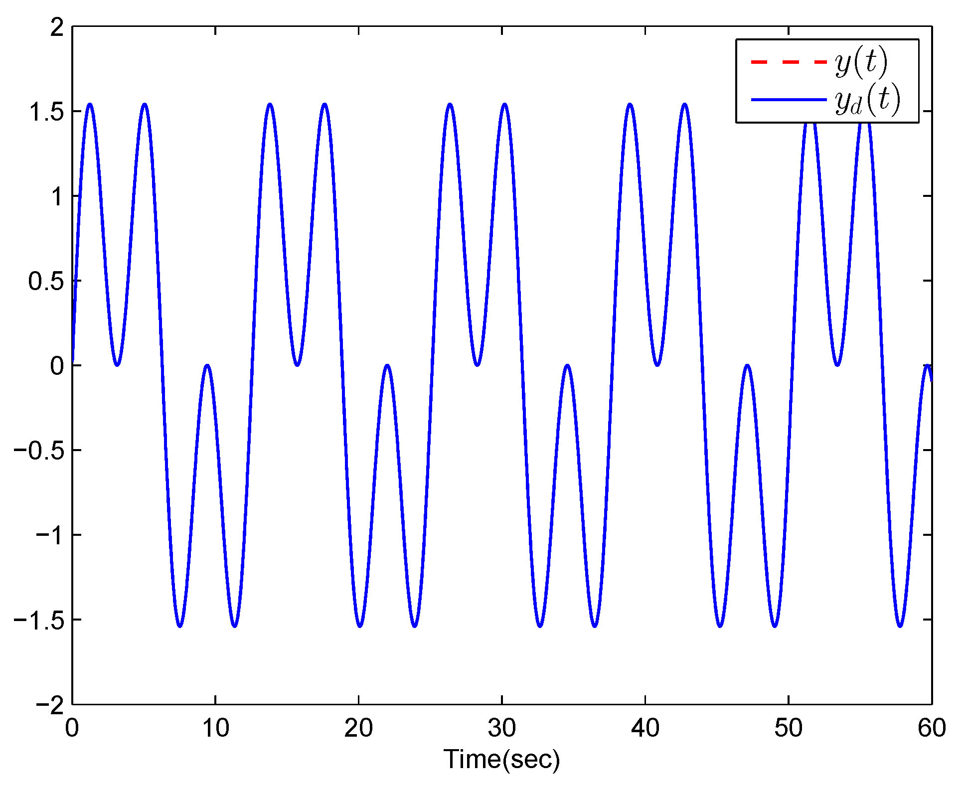
where σ ( t ) { 1 , 2 } , f 11 = x 1 ( 1 + x 1 2 ) , f 12 = x 1 2 x 2 , f 21 = x 2 , f 22 = x 2 0.01 x 3 , f 31 = ( 1 + x 3 2 ) u x 1 2 x 3 , f 32 = x 3 2 x 2 2 u , g 11 = s i n x 1 , g 12 = x 1 + x 1 s i n x 2 , g 21 = 0.1 x 1 2 , g 22 = 0.1 x 1 2 s i n x 2 , g 31 = x 3 2 s i n x 2 , g 32 = 0.01 x 1 s i n x 2 x 3 2 , ψ 11 = 0.2 ( x 1 2 + x 2 2 ) , ψ 21 = 0.5 x 2 2 , ψ 21 = 2 x 1 2 , ψ 22 = x 1 2 x 2 , ψ 31 = x 1 2 , ψ 32 = x 1 2 x 3 , where x 1 , x 2 and x 3 are the states, y is the output, u = H ( v ) defined in (5) with μ 1 = 1 , μ 2 = 2 , β = 1 , χ = 2 . The aim is to design a virtual control signal v ¯ ( t ) such that all the signals are SGUUB in probability and the output y follows the reference signal y d = 0.5 s i n ( t ) + s i n ( 0.5 t ) under arbitrary switching.
By Remark 2, to design the fuzzy controller, the membership functions are constructed as follows:
μ F i 1 ( x i ) = e x p ( ( x i + 1 ) 2 / 2 ) ; μ F i 2 ( x i ) = e x p ( ( x i + 1.5 ) 2 / 2 ) ;
μ F i 3 ( x i ) = e x p ( ( x i + 0.5 ) 2 / 2 ) ; μ F i 4 ( x i ) = e x p ( ( x i ) 2 / 2 ) ; μ F i 5 ( x i ) = e x p ( ( x i 1 ) 2 / 2 ) ;
μ F i 6 ( x i ) = e x p ( ( x i 1.5 ) 2 / 2 ) ; μ F i 7 ( x i ) = e x p ( ( x i 0.5 ) 2 / 2 ) , i = 1 , 2 , 3 .
From Theorem 1, let
α i = k i z i 1 2 a i 2 θ ^ i z i 3 Y i T ( X i ) Y i ( X i ) + x i + 1 0 , i = 1 , 2 , k = 1 , 2 , 3 , v = N ( ι ) v ¯ + v 0 v ¯ = k 3 z 3 1 2 a 3 2 θ ^ 3 z 3 3 Y 3 T ( X 3 ) Y 3 ( X 3 ) , N ( ι ) = ι 2 c o s ( ι ) , ι ˙ = γ v ¯ z n 3 , θ ^ ˙ i = γ i θ ^ i + λ i 2 a i 2 z i 6 Y i T ( X i ) Y i ( X i ) , i = 1 , 2 , 3
where z 1 = x 1 y d , z 2 = x 2 α 1 , z 3 = x 3 α 2 , X 1 = [ x 1 , y d , y ˙ d ] T , X 2 = [ x ¯ 2 T , θ ^ 1 , y ¯ d ( 2 ) T ] T , X 3 = [ x ¯ 3 T , θ ^ 1 , θ ^ 2 , y ¯ d ( 3 ) T ] T . The parameters are chosen as follows: k 1 = 2 , k 2 = 3 , k 3 = 2 , a 1 = a 2 = a 3 = 3 , λ 1 = 5 , λ 2 = 3 , λ 3 = 1 , γ 1 = 0.6 , γ 2 = 2 , γ 3 = 2 , x 2 0 = x 3 0 = v 0 = 0 , γ = 120 . The simulation is run under [ x 1 ( 0 ) , x 2 ( 0 ) , x 3 ( 0 ) ] T = [ 0 , 0.2 , 2 ] T , [ θ ^ 1 ( 0 ) , θ ^ 2 ( 0 ) , θ ^ 3 ( 0 ) ] T = [ 0.3 , 0.3 , 3 ] T .
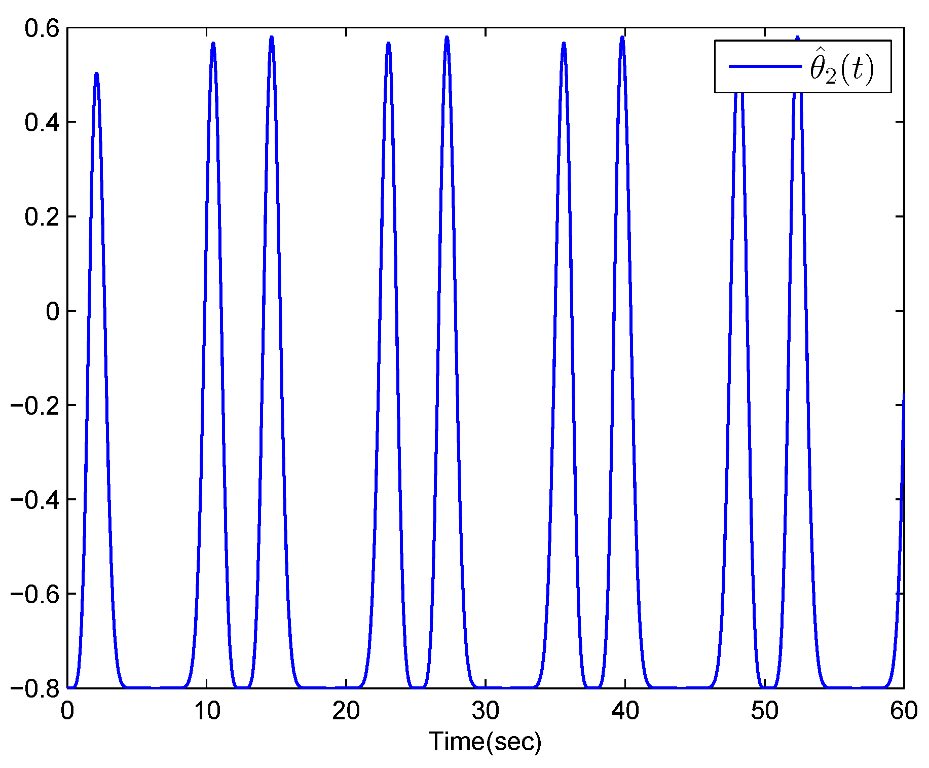
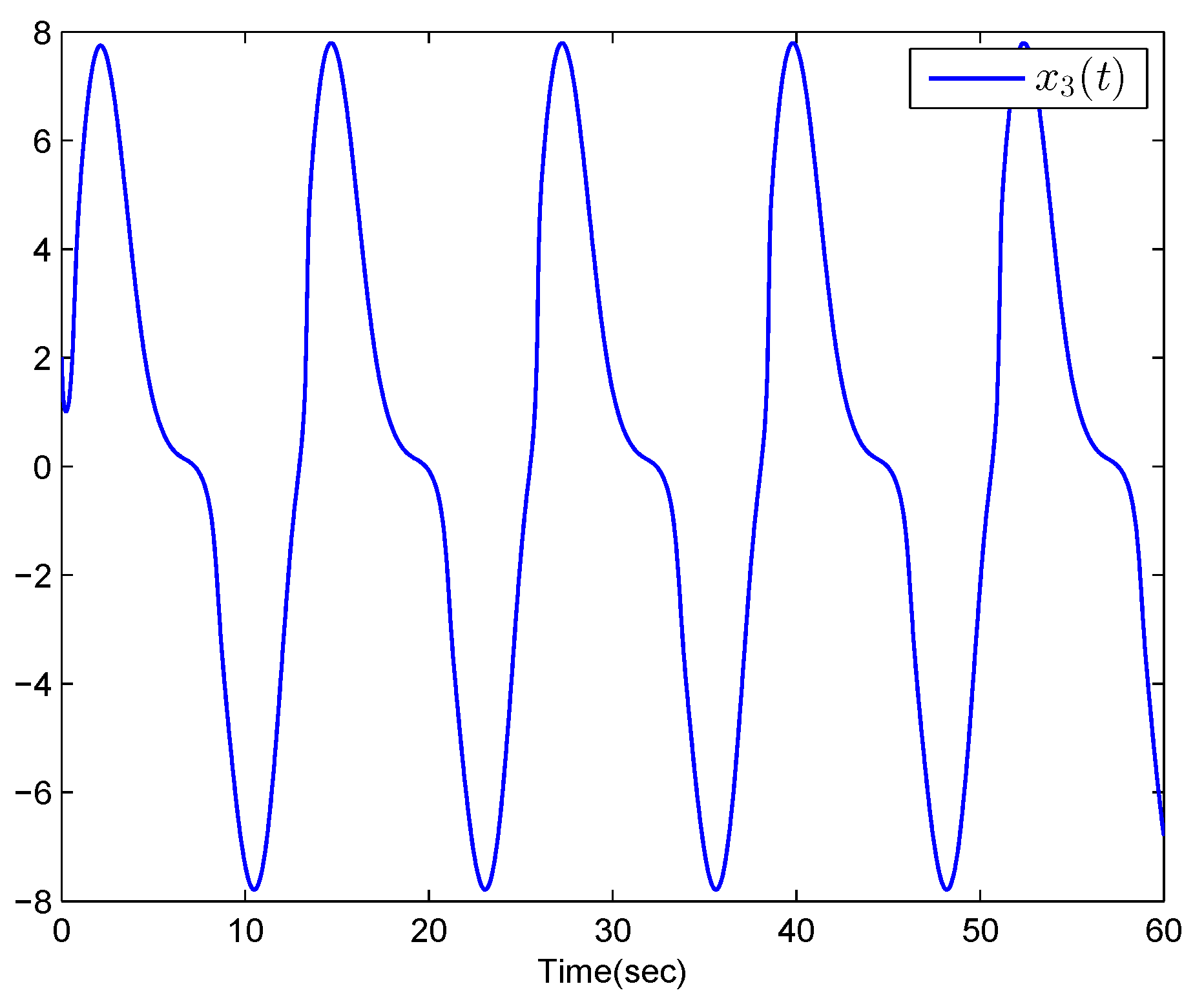
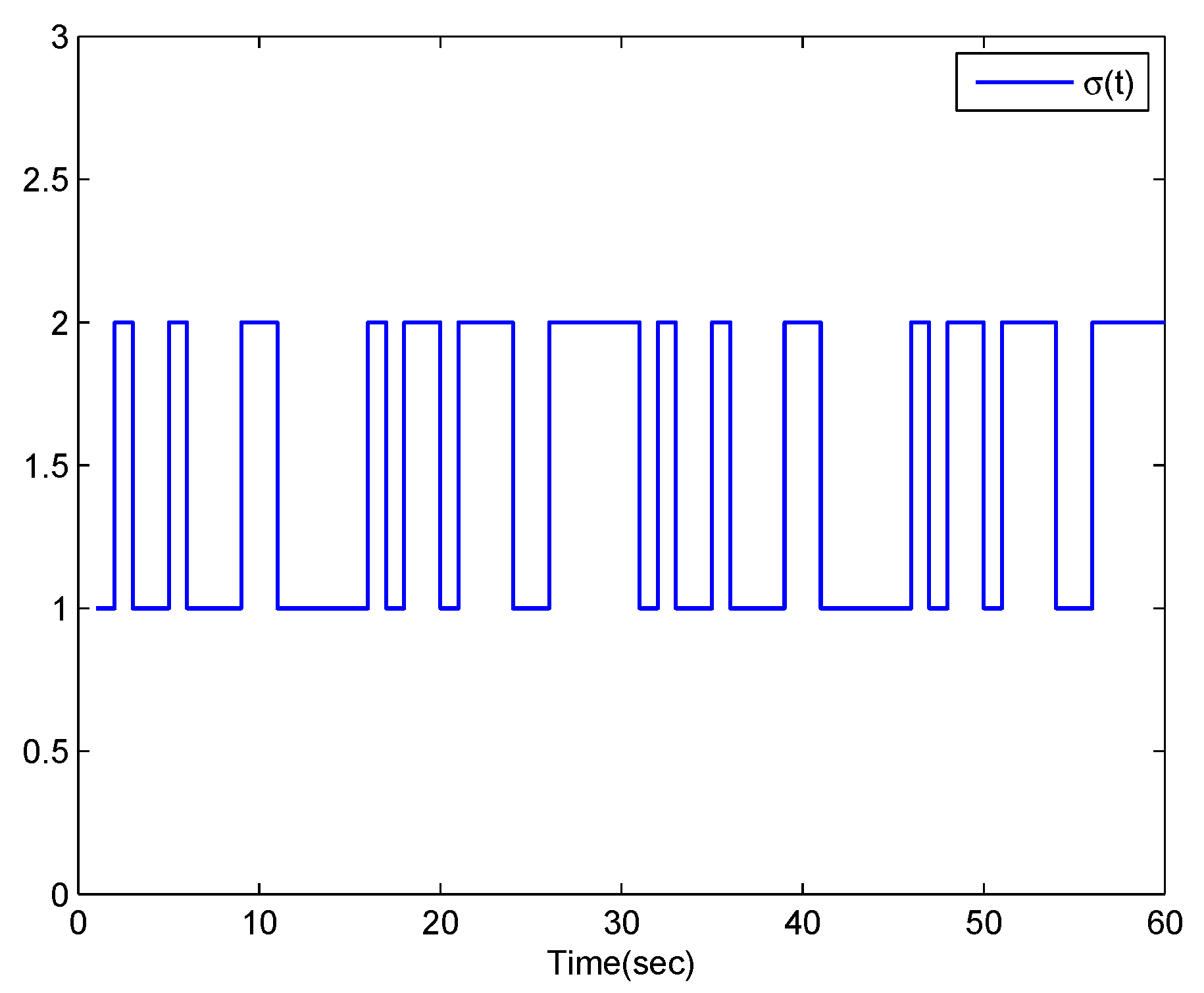
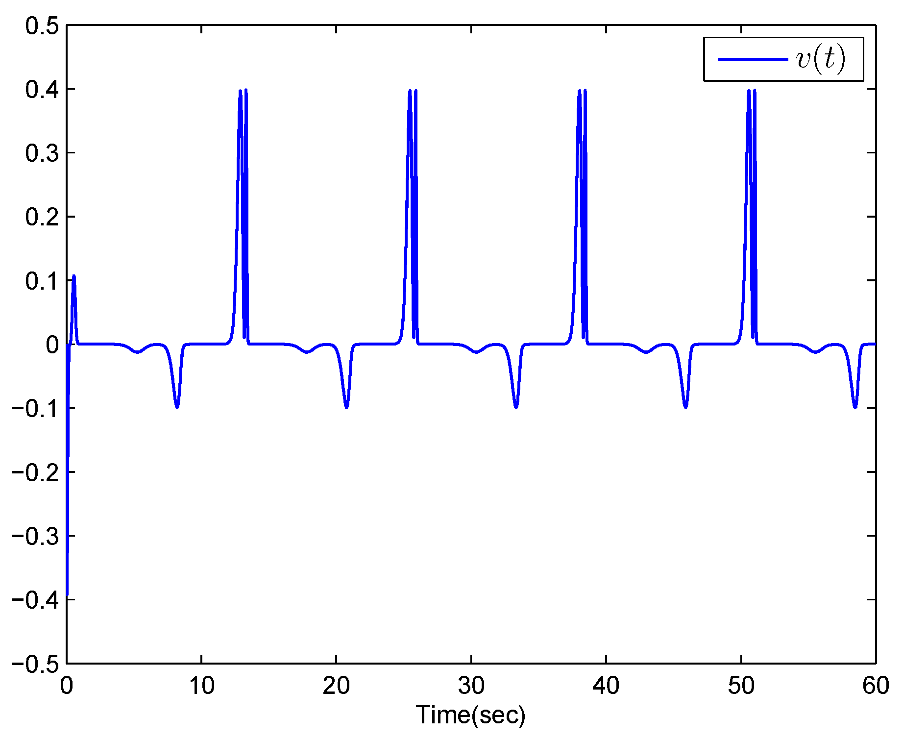
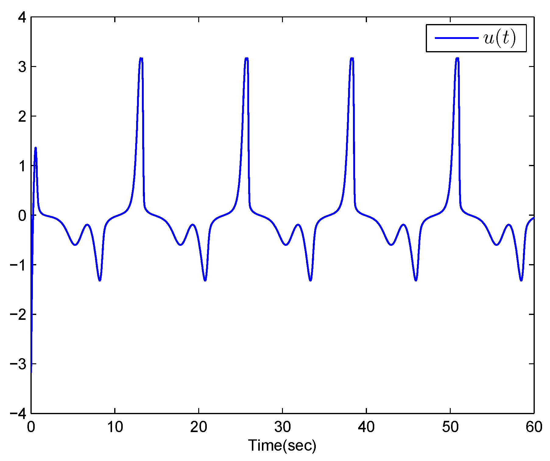
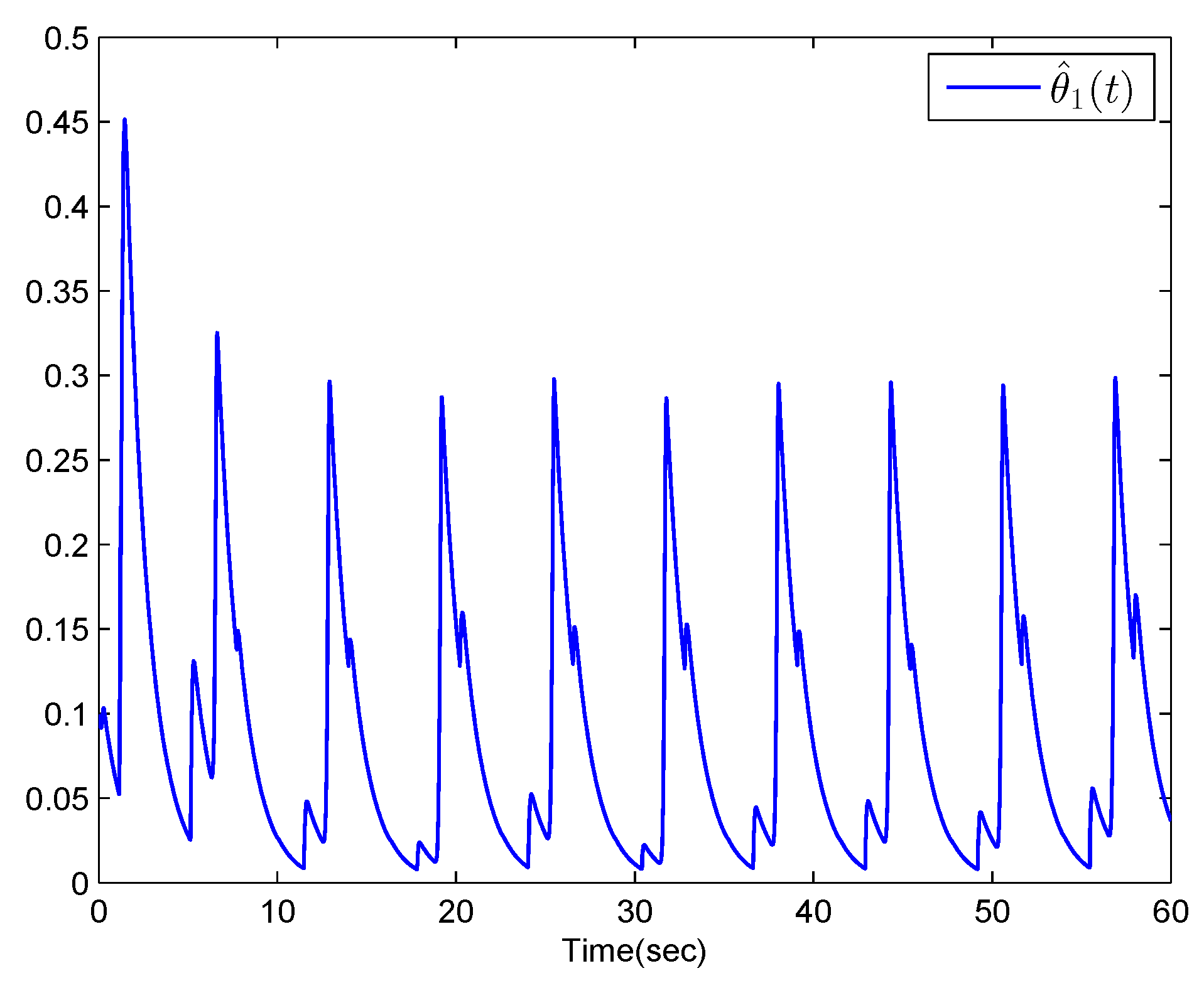
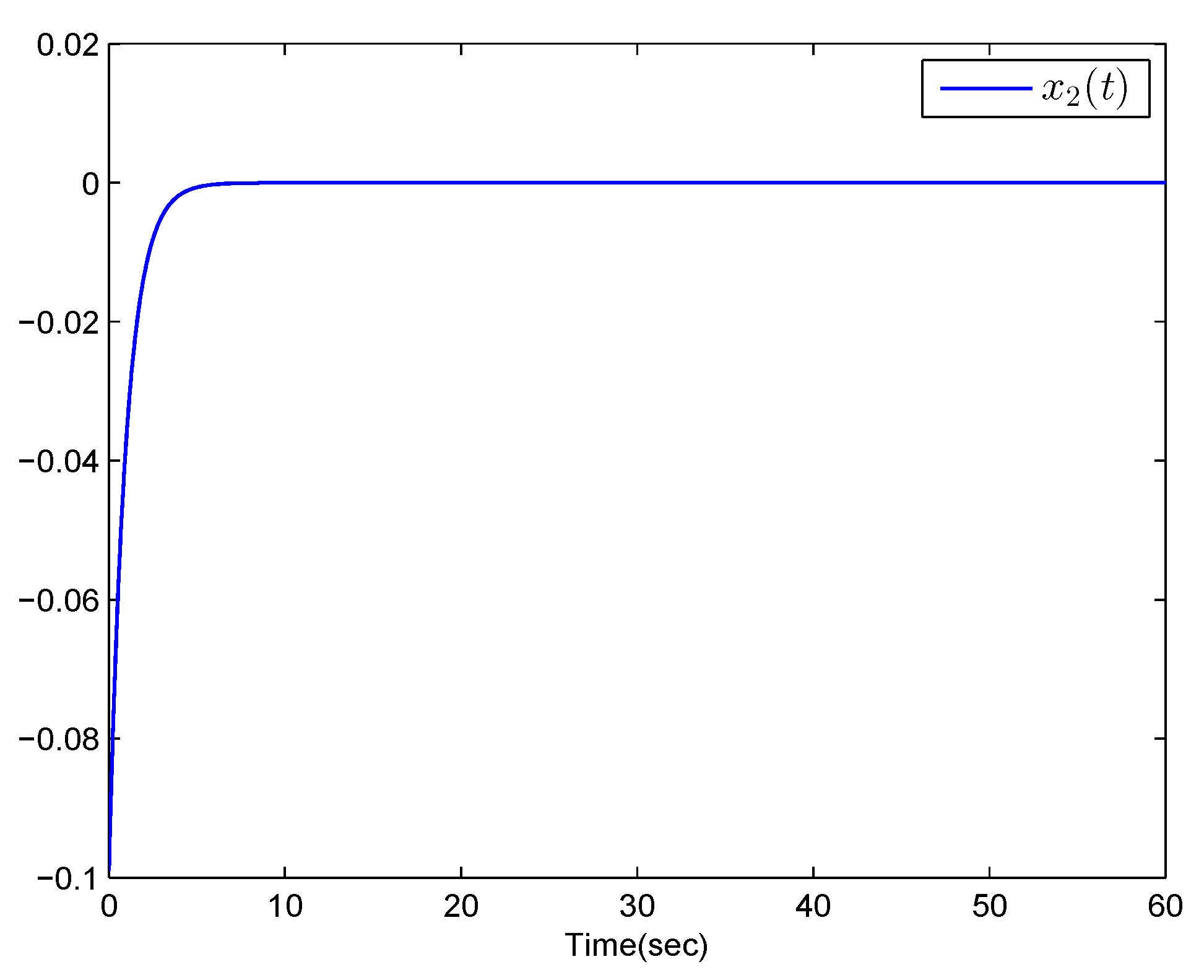
Figure 1, Figure 2, Figure 3, Figure 4, Figure 5, Figure 6, Figure 7, Figure 8 and Figure 9 display the simulation results. The trajectories of system output y and reference signal y d are shown in Figure 1. It can be seen that a good tracking performance can be obtained. Figure 2, Figure 3 and Figure 4, respectively, show the trajectories of the adaptive parameters θ ^ 1 , θ ^ 2 and θ ^ 3 . The boundness of state variables x 2 and x 3 is displayed in Figure 5 and Figure 6. Figure 7 shows the evolution of switching signal σ ( t ) . Figure 8 and Figure 9, respectively, show the trajectories of control input v ( t ) and system input u ( t ) . From the simulation results, it can be clearly seen that the proposed adaptive control method can guarantee that all the signals of the closed-loop systems remain bounded and the output tracking error converges to a small neighborhood of zero.
Example 2. 
Consider the continuous stirred tank reactor with two modes feed stream [45], and an unknown Bouc–Wen hysteresis u defined in (5). Therefore, the following switched stochastic nonlinear system is considered:
d x 1 = ( f 1 , σ ( t ) ( x 1 , x 2 ) d t + ψ 1 , σ ( t ) T ( x 1 , x 2 ) d w , d x 2 = u d t , y = x 1 , σ ( t ) { 1 , 2 } ,
where f 1 , 1 ( x 1 , x 2 ) = x 2 x 1 + s i n x 1 , f 1 , 2 ( x 1 , x 2 ) = x 2 x 1 2 x 2 , ψ 1 , 1 ( x 1 , x 2 ) = 0.5 x 1 2 + x 2 2 , ψ 1 , 2 ( x 1 , x 2 ) = 0.5 x 2 .
The fuzzy membership functions are chosen in Example 1, and the reference signal is y d ( t ) = s i n ( 0.5 t ) + s i n ( 1.5 t ) . In the following, designed parameters and initial condition are μ 1 = 1 , μ 2 = 2 , β = 2 , χ = 1 , k 1 = 2 , k 2 = 4 , a 1 = 3 , a 2 = 2 , λ 1 = 5 , λ 2 = 3 , γ 1 = γ 2 = 1 , x 2 0 = v 0 = 0 , [ x 1 ( 0 ) , x 2 ( 0 ) ] T = [ 0 , 0.3 ] T , [ θ ^ 1 ( 0 ) , θ ^ 2 ( 0 ) ] T = [ 0.2 , 0.3 ] T .
Similarly, based on Theorem 1, the simulation results are presented in Figure 10, Figure 11, Figure 12, Figure 13, Figure 14 and Figure 15. Figure 10 shows the evolution of switching signal σ ( t ) . Figure 11 presents the system output y and the reference signal y d . Figure 12, Figure 13 and Figure 14 show that the state variable and adaptive parameters are bounded, respectively. Figure 15 shows the trajectories of control input v ( t ) . Both analytic results and simulation results indicate that the output signal tracks the reference signal, and all the signals remain bounded.

5. Conclusions

An adaptive tracking control problem was proposed for nonlinear stochastic switched systems with unknown hysteresis. The stochastic noises and the unknown hysteresis have been coexisting. By introducing an auxiliary virtual controller and a Nussbaum function, the unknown direction hysteresis is addressed. The proposed scheme can guarantee that all the closed-loop system signals are SGUUB in probability and that the tracking error converges to a small neighborhood of the origin. Our future work will focus on saturation nonlinearity in both control design and stability analysis for switched stochastic nonlinear systems.

Author Contributions

Conceptualization and Methodology, Y.L.; Writing—original draft and Data curation, X.W.; Funding acquisition, Writing—review and editing, Y.L. All authors have read and agreed to the published version of the manuscript.

Funding

This work was supported by the National Natural Science Foundation of China (No. 61972236), Shandong Provincial Natural Science Foundation (No. ZR2022MF233).

Data Availability Statement

The data presented in this study are available on request from the corresponding author.

Acknowledgments

The authors are grateful to the referees for their constructive suggestions.

Conflicts of Interest

The authors declare no conflict of interest.

References

  1. Li, Z.; Wen, C.; Soh, Y. Switched controllers and their applications in bilinear systems. Automatica 2001, 37, 477–481. [Google Scholar] [CrossRef]
  2. Homaee, O.; Zakariazadeh, A.; Jadid, S. Real-time voltage control algorithm with switched capacitors in smart distribution system in presence of renewable generations. Int. J. Electr. Power 2014, 54, 187–197. [Google Scholar] [CrossRef]
  3. Jeon, D.; Tomizuka, M. Learning hybrid force and position control of robot manipulators. IEEE Trans. Robot. Autom. 1993, 9, 423–431. [Google Scholar] [CrossRef]
  4. Zhao, J.; Hill, D.; Liu, T. Synchronization of complex dynamical networks with switching topology: A switched system point of view. Automatica 2009, 45, 2502–2511. [Google Scholar] [CrossRef]
  5. Yuan, X.; Chen, B.; Lin, C. Fuzzy adaptive fuzzy output-feedback tracking control for nonlinear strict-feedback systems in prescribed finite time. J. Frankl. Inst. 2021, 358, 7309–7332. [Google Scholar] [CrossRef]
  6. Zhao, D.; Ouyang, X.; Zhao, N.; Zhang, F. Event-triggered low-computation adaptive output-feedback fuzzy tracking control of uncertain nonlinear systems. ISA Trans. 2023, 144, 86–95. [Google Scholar] [CrossRef]
  7. Zhao, X.; Zheng, X.; Niu, B.; Liu, L. Adaptive tracking control for a class of uncertain switched nonlinear systems. Automatica 2015, 52, 185–191. [Google Scholar] [CrossRef]
  8. Xiong, Y.; Wu, Y.; Li, S.; Xiang, Z. Adaptive fuzzy output feedback fault-tolerant tracking control of switched uncertain nonlinear systems with sensor faults. J. Frankl. Inst. 2021, 358, 5771–5794. [Google Scholar] [CrossRef]
  9. Zhang, L.; Zhuang, S.; Shi, P. Non-weighted quasi-time-dependent H filtering for switched linear systems with persistent dwell-time. Automatica 2015, 54, 201–209. [Google Scholar] [CrossRef]
  10. Zeng, D.; Liu, Z.; Chen, C.; Zhang, T. Event-triggered fuzzy adaptive control of nonlinear switched systems with predefined accuracy and mismatched switching. Fuzzy Set Syst. 2022, 443, 283–307. [Google Scholar] [CrossRef]
  11. Wu, Y.; Zhang, G.; Wu, L. Command filter-based adaptive fuzzy switching event-triggered control for non-affine nonlinear systems with actuator faults. Inf. Sci. 2023, 638, 118991. [Google Scholar] [CrossRef]
  12. Zhao, J.; Hill, D. On stability, L2-gain and H control for switched systems. Automatica 2008, 44, 1220–1232. [Google Scholar] [CrossRef]
  13. Muller, M.; Liberzon, D. Input/output-to-state stability and state-norm estimators for switched nonlinear systems. Automatica 2012, 48, 2029–2039. [Google Scholar] [CrossRef]
  14. Lin, H.; Antsaklis, P. Stability and stabilizability of switched linear systems: A survey of recent results. IEEE Trans. Autom. Control 2009, 54, 308–322. [Google Scholar] [CrossRef]
  15. Komurcugil, H.; Ozdemir, S.; Sefa, I.; Altin, N.; Kukrer, O. Sliding-mode control for single-phase grid-connected LCL-filtered vsi with double-band hysteresis scheme. IEEE Trans. Ind. Electron. 2016, 63, 864–873. [Google Scholar] [CrossRef]
  16. Tan, X.; Baras, J. Modeling and control of hysteresis in magnestrictive actuators. Automatica 2004, 40, 1469–1480. [Google Scholar] [CrossRef]
  17. Wen, C.; Zhou, J. Decentralized adaptive stabilization in the presence of unknown backlash-like hysteresis. Automatica 2007, 43, 426–440. [Google Scholar] [CrossRef]
  18. Chen, G.; Dong, J. Approximate optimal adaptive prescribed performance control for uncertain nonlinear systems with feature information. IEEE Trans. Syst. Man Cybern. Syst. 2024, 54, 2298–2308. [Google Scholar] [CrossRef]
  19. Ebeigbe, D.; Nguyen, T.; Richter, H.; Simon, D. Robust Regressor-free control of rigid robots using function approximations. IEEE Trans. Control Syst. Technol. 2020, 28, 1433–1446. [Google Scholar] [CrossRef]
  20. Yang, Y.; Liu, G.; Li, Q.; Ahn, G. Multiple adaptive fuzzy Nussbaum-type functions design for stochastic nonlinear systems with fixed-time performance. Fuzzy Set Syst. 2024, 476, 108767. [Google Scholar] [CrossRef]
  21. Oksendal, B. Stochastic Differential Equations: An Introduction with Applications, 5th ed.; Springer: New York, NY, USA, 2000. [Google Scholar] [CrossRef]
  22. Yu, Z.; Li, S.; Yu, Z.; Li, F. Adaptive neural output feedback control for nonstrict-feedback stochastic nonlinear systems with unknown backlash-like hysteresis and unknown control directions. IEEE Trans. Neural Netw. Learn. Syst. 2018, 29, 1147–1160. [Google Scholar] [CrossRef]
  23. Wang, F.; Liu, Z.; Zhang, Y.; Chen, C. Adaptive fuzzy control for a class of stochastic pure-feedback nonlinear systems with unknown hysteresis. IEEE Trans. Fuzzy. Syst. 2016, 24, 140–152. [Google Scholar] [CrossRef]
  24. Deng, H.; Krstic, M. Output-feedback stochastic nonlinear stabilization. IEEE Trans. Autom. Control 1999, 44, 328–333. [Google Scholar] [CrossRef]
  25. Deng, H.; Krstic, M. Output-feedback stabilization of stochastic nonlinear systems driven by noise of unknown covariance. Syst. Control Lett. 2000, 39, 173–182. [Google Scholar] [CrossRef]
  26. Feng, G. A survey on analysis and design of model-based fuzzy control systems. IEEE Trans. Fuzzy Syst. 2006, 14, 676–697. [Google Scholar] [CrossRef]
  27. Li, D.; Dong, J. Fuzzy control based on reinforcement learning and subsystem error derivatives for strict-feedback systems with an observer. IEEE Trans. Fuzzy Syst. 2023, 31, 2509–2521. [Google Scholar] [CrossRef]
  28. Namadchian, Z.; Rouhani, M. Adaptive prescribed performance neural network control for switched stochastic pure-feedback systems with unknown hysteresis. Neurocomputing 2021, 429, 151–165. [Google Scholar] [CrossRef]
  29. Liu, S.; Zhang, L.; Niu, B.; Zhao, X.; Ahmad, A. Adaptive neural finite-time hierarchical sliding mode control of uncertain under-actuated switched nonlinear systems with backlash-like hysteresis. Inf. Sci. 2022, 599, 147–169. [Google Scholar] [CrossRef]
  30. Xu, S.; Wang, Z.; Fan, X.; Xiong, B. Experimental investigations of hypersonic inlet unstart/restart process and hysteresis phenomenon caused by angle of attack. Aerosp. Sci. Technol. 2023, 126, 107621. [Google Scholar] [CrossRef]
  31. Hao, S.; Pan, Y.; Zhu, Y.; Cao, L. Event-based adaptive tracking control for robotic systems with deferred position constraints and unknown backlash-like hysteresis. ISA Trans. 2023, 142, 289–298. [Google Scholar] [CrossRef]
  32. Zhang, C.; Zhou, M.; Nie, L.; Zhang, X.; Su, C. Prandtl-Ishlinskii model based event-triggered prescribed control: Design and application to piezoelectric-driven micropositioning stage. Mech. Syst. Signal Process. 2023, 200, 110562. [Google Scholar] [CrossRef]
  33. Mayergoyz, I. The Preisach Model for Hysteresis; Springer: Berlin, Germany, 1991. [Google Scholar]
  34. Wang, G.; Chen, G. Identification of piezoelectric hysteresis by a novel Duhem model based neural network. Sens. Actuators A Phys. 2017, 264, 282–288. [Google Scholar] [CrossRef]
  35. Ibrir, S.; Su, C. Adaptive stabilization of a class of feedforward nonlinear systems subject to unknown backlash-hysteresis inputs. IEEE Trans. Control Syst. Technol. 2017, 25, 1180–1192. [Google Scholar] [CrossRef]
  36. Chen, X.; Li, S.; Wang, R.; Xiang, Z. Event-Triggered output feedback adaptive control for nonlinear switched interconnected systems with unknown control coefficients. Appl. Math. Comput. 2023, 445, 127854. [Google Scholar] [CrossRef]
  37. Zhao, Z.; Liu, Z.; He, W.; Hong, K.; Li, H. Boundary adaptive fault-tolerant control for a flexible Timoshenko arm with backlash-like hysteresis. Automatica 2021, 130, 109690. [Google Scholar] [CrossRef]
  38. Zhu, Z.; Pan, Y.; Zhou, Q.; Lu, C. Event-triggered adaptive fuzzy control for stochastic nonlinear systems with unmeasured states and unknown backlash-like hysteresis. IEEE Trans. Fuzzy Syst. 2021, 29, 1273–1283. [Google Scholar] [CrossRef]
  39. Zhao, Z.; Zhang, J.; Liu, Z.; Mu, C.; Hong, K. Adaptive neural network control of an uncertain 2-DOF helicopter with unknown backlash-like hysteresis and output constraints. IEEE Trans. Neural Netw. Learn. Syst. 2023, 34, 10018–10027. [Google Scholar] [CrossRef]
  40. Fu, C.; Wang, Q.; Yu, J.; Lin, C. Neural network-based finite-time command filtering control for switched nonlinear systems with backlash-like hysteresis. IEEE Trans. Neural Netw. Learn. Syst. 2021, 32, 3268–3273. [Google Scholar] [CrossRef] [PubMed]
  41. Ji, H.; Xi, H. Adaptive output-feedback tracking of stochastic nonlinear systems. IEEE Trans. Autom. Control 2006, 51, 355–360. [Google Scholar] [CrossRef]
  42. Deng, H.; Kristic, M. Stochastic nonlinear stabilization-I: A backstepping design. Syst. Control Lett. 1997, 32, 143–150. [Google Scholar] [CrossRef]
  43. Zhou, J.; Wen, C.; Li, T. Adaptive output feedback control of uncertain nonlinear systems with hysteresis nonlinearity. IEEE Trans. Autom. Control. 2012, 57, 2627–2633. [Google Scholar] [CrossRef]
  44. Takagi, T.; Sugeno, M. Fuzzy identification of systems and its applications to modeling and control. IEEE Trans. Syst. Man Cybern. 1985, 15, 116–132. [Google Scholar] [CrossRef]
  45. Niu, B.; Qin, T.; Fan, X. Adaptive neural network tracking control for a class of switched stochastic pure-feedback nonlinear systems with backlash-like hysteresis. Int. J. Syst. Sci. 2016, 47, 3378–3393. [Google Scholar] [CrossRef]
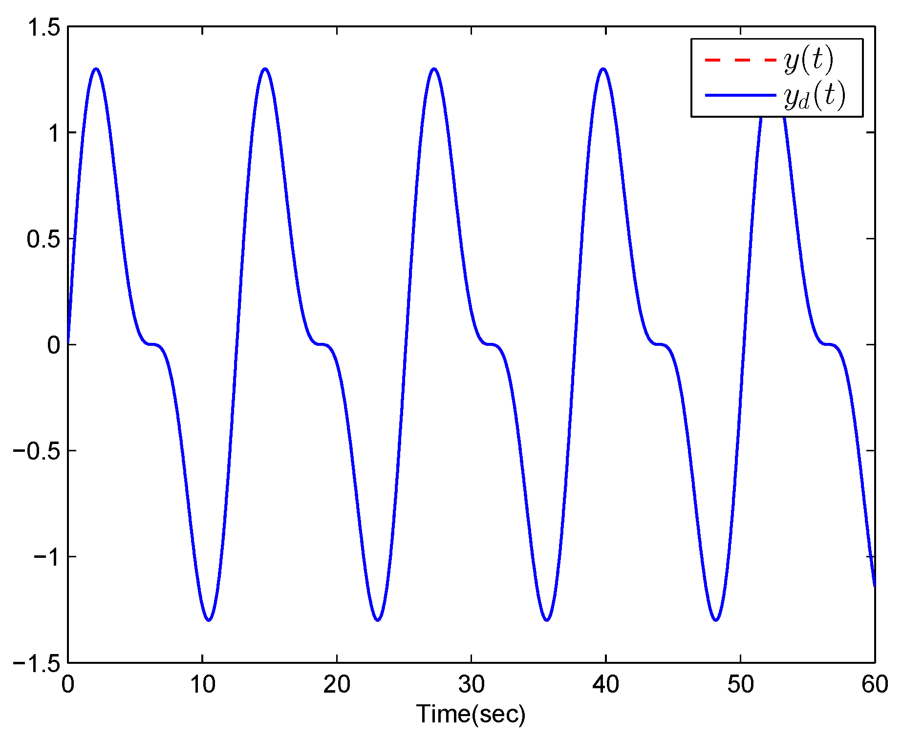
Figure 1. Trajectories of y ( t ) and y d ( t ) .
Mathematics 12 01070 g001
Figure 2. Adaptive parameter θ ^ 1 ( t ) .
Mathematics 12 01070 g002
Figure 3. Adaptive parameter θ ^ 2 ( t ) .
Mathematics 12 01070 g003
Figure 4. Adaptive parameter θ ^ 3 ( t ) .
Mathematics 12 01070 g004
Figure 5. State variable x 2 ( t ) .
Mathematics 12 01070 g005
Figure 6. State variable x 3 ( t ) .
Mathematics 12 01070 g006
Figure 7. Switching signal σ ( t ) .
Mathematics 12 01070 g007
Figure 8. Control input signal v ( t ) .
Mathematics 12 01070 g008
Figure 9. System input u ( t ) .
Mathematics 12 01070 g009
Figure 10. Switching signal σ ( t ) in Example 2.
Mathematics 12 01070 g010
Figure 11. Trajectories of y ( t ) and y d ( t ) in Example 2.
Mathematics 12 01070 g011
Figure 12. Adaptive parameter θ ^ 1 ( t ) in Example 2.
Mathematics 12 01070 g012
Figure 13. Adaptive parameter θ ^ 2 ( t ) in Example 2.
Mathematics 12 01070 g013
Figure 14. State variable x 2 ( t ) in Example 2.
Mathematics 12 01070 g014
Figure 15. Control input signal v ( t ) in Example 2.
Mathematics 12 01070 g015
Disclaimer/Publisher’s Note: The statements, opinions and data contained in all publications are solely those of the individual author(s) and contributor(s) and not of MDPI and/or the editor(s). MDPI and/or the editor(s) disclaim responsibility for any injury to people or property resulting from any ideas, methods, instructions or products referred to in the content.