Turing Instability and Spatial Pattern Formation in a Model of Urban Crime

Abstract

A nonlinear crime model is generalized by introducing self- and cross-diffusion terms. The effect of diffusion on the stability of non-negative constant steady states is applied. In particular, the cross-diffusion-driven instability, called Turing instability, is analyzed by linear stability analysis, and several Turing patterns driven by the cross-diffusion are studied through numerical investigations. When the Turing–Hopf conditions are satisfied, the type of instability highlighted in the ODE model persists in the PDE system, still showing an oscillatory behavior.

1. Introduction

Crime and criminal activities have a wide influence on society and its development. Criminal activities not only endanger the safety of the population, but also slow down the economic process of the community. Various factors contribute to committing crime, for example, immigration of criminals and the learning of criminal behavior through interactions between criminally predisposed individuals and delinquent individuals. It is often observed that contact with criminal and delinquent individuals can produce criminal behaviors in the individuals involved and stimulate them to commit a crime [1]. Numerous scholars have conducted empirical and practical studies on various aspects of crime growth and prevention. Just as some examples, in [2], the author examined and discussed the trend and models of robbery and its various consequences in Ghana between 1982 and 1983; in [3], the authors studied the socioeconomic and demographic factors that influenced the spread of crime in Germany and found that higher economic well-being corresponds to higher crime rates.

Economic investigations into the importance of the spread of crime in society took off in the late 1960s when several economists (a small sampling includes [3,4,5,6]) turned their attention to the field of crime. In [4], a model, based on the theory of deterrence, predicted how changes in the probability and severity of sanctions may affect crime. In [3], considering a time allocation model, a descriptive analysis of crime and the potential factors contributing to crime in Germany are given. In [5], the relationship between crime and geographic space is explored, in relation to property crimes and violence, using population density in United States. The containment of the spread of crime in urban societies remains a major challenge. Empirical evidence suggests that crimes may be recurrent and proliferate if left unchecked; therefore, any kind of investigation can provide information or tools that may prove useful in its prevention and control. Mathematical modeling is a powerful tool that has been employed and developed to examine the spread of crime. One of the main targets to be achieved is to understand the conditions that allow crime to disappear from or persist within a community. Recent research has highlighted that applied mathematics may help us to understand criminal activity. Differential equations, the self-exciting point process, agent-based modeling and adversarial evolutionary games are different approaches to modeling crime activity. The study of the dynamics of the spread of crime is not untouched by predator–prey dynamics. It is a well-known fact that the interaction of criminally minded individuals with non-criminal individuals can be represented as the interaction of a predatory population with a population of prey. There are various useful studies that have dealt with quantitative models of crime which are able to represent the behavior of interacting populations in relative societies [7,8,9,10]. In particular, in [7], the authors analyzed a system of three ordinary differential equations to account for the time evolution of three sociological species, called owners, criminals and security guards. In [8], a model is constructed, based on the well-known predator–prey model, to analyze the interaction between the criminal population and the non-criminal one. Furthermore, a law enforcement term, an important part of any country’s political and social systems, is incorporated in the model, and its effect is studied. The elimination or the persistence of crime is discussed via two parameters, law enforcement and the saturation constant. In [10], a diffusion-type differential equations model that captures the dynamics that describe the behavior in time of serious and minor crime is studied, and numerical solutions are compared with the crime data for the Greater Manchester area, highlighting a satisfactory agreement. In [11], a deterministic mathematical model based on nonlinear ordinary differential equations, considering education programs as a valid means of estimating the population-level impact on crime prevalence, is studied. The model is fitted with prison data (reported from July 2021 to June 2022) by the State of Illinois in the United States.

In recent years, there has been increasing interest in developing mathematical tools to understand and predict the spatial patterns of urban crime [12,13,14,15,16,17,18,19]. Several researchers have determined suitable models for analyzing intervention strategies that decrease delinquent behavior and promote social development. As a first modeling step, the population is spatially distributed over a geographical region in a homogeneous manner; only temporal variability is considered under the scheme. The formation of crime clusters suggests that criminally minded individuals do not always distribute themselves uniformly in space and time but often congregate in small clusters. Many criminal events, such as those relating to drugs, robberies, burglaries, etc., often originate from situations of aggregation or particular distributions. In fact, the composition or the distribution of the population has a relevant impact on the propagation of crime within the society. Although criminality is an aspect now present in all societies, some places have a greater propensity for crime than others. For example, data on residential burglaries show high-crime places bounded by low-crime areas. Several studies indicate that crime in a place involves more crime in that and neighboring places, leading to residential burglary hotspots; this finding emerged from real data. The observation that residential burglaries are not spatially homogeneously distributed and that certain neighborhoods have a greater propensity for crime than others led Short et al. [15,16,20] to study the dynamics of residential burglary hotspots. In particular, starting from the discrete system, the authors derived a continuum model; the two approaches are in good quantitative agreement for large system sizes. Through a linear stability analysis, they found the parameter values leading to the formation of stable hotspots.

Among the various approaches that can be found in the literature to describe the distribution of different species, populations or groups of individuals in various contexts, in space at different times, and due to local interaction and diffusion, are reaction–diffusion models. In particular, reaction–diffusion equations are often used to model spatial effects in many fields of applied mathematics, such as ecology [21,22,23], biology and medicine [24], economics [25], epidemiology [26,27] and social sciences [28,29]. Though these various fields and systems may seem completely different, the mathematics describing the pattern formation in them is surprisingly similar. The study of reaction–diffusion systems may be faced using numerical or analytical methods from the theory of partial differential equations and dynamic systems. In [30], the authors considered models representing social interactions between ordinary individuals, drug users/dealers and policemen, starting from a model proposed by Epstein in [31] and introducing two modified models. They take into account an additional cross–diffusion term and some logistic effects. In the above paper, they analyze the Turing instability from an analytical point of view and increase some patterns, choosing the values of the parameters close enough to those used in [31].

In this paper, we follow this line of research, starting from the continuous model of crime introduced in [12], which incorporates the law enforcement term. In [12], the authors developed a model based on the prey–predator interaction in order to study the dynamics between the criminal and non-criminal individuals living in a specific society. More precisely, a predator–prey model with a Holling type II functional response and logistic growth rate in the non-criminal population is introduced. The considered functional response is characterized by a decelerating intake rate, which is derived from assuming that the criminally minded individuals are prevented by their capacity from victimizing the non-criminal individuals. Moreover, as law enforcement is the appropriate measure for controlling the crime rate in a community, in [12], it is considered in the criminally minded population. The role of population density in the reduction or increase in crime has been the subject of debate for a long time [32]. Whenever social, political, economic and environmental aspects are considered and observed, it is easy to find the interaction between two different and contrasting mentalities (as, for example, in the case in question: non-criminal mentality and criminal mentality) which, among other things, contributes to the degradation of society. In a given place or country, modeling how different mentalities influence criminality can be a valid starting point for scholars in the field. The basic assumption in [12] is that the only way for new criminally minded individuals to emerge is their interactions with existing criminally minded individuals. In this line of research, we place our study. $C_P\left(t\right)$ denotes the criminally minded population density and $N_P\left(t\right)$ the non-criminally minded population density at time t. In [12], the following system is introduced:

$$\left\{\begin{array}{c}{\displaystyle \frac{d{N}_P}{dt}=\mu \left(1-\frac{N_P}{K}\right)N_P-a\frac{N_P{C}_P}{\sigma +N_P},}\hfill \\ \\ {\displaystyle \frac{d{C}_P}{dt}=-\gamma C_P+b\frac{N_P{C}_P}{\sigma +N_P}-L_C{C}_P.}\hfill \end{array}\right.$$

(1)

The parameters $\mu ,a,b,\gamma ,\sigma ,K$ and $L_C$, all positive, are defined as follows:

• $\mu$: per capita growth rate (the intrinsic rate of increase) of non-criminal individuals in the absence of criminal ones $C_P$;
• a: the rate at which $C_P$ victimizes $N_P$ (i.e., maximum capture/predation rate);
• $\gamma$: natural mortality rate of $C_P$ in the absence of non-criminal individuals $N_P$;
• b: conversion rate of non-criminal population $N_P$ into criminal population $C_P$;
• $\sigma$: the half saturation constant (the value at which the half of the rate constant (a) is attained);
• K: the carrying capacity of the non-criminal population in the absence of a criminal one;
• $L_C$: measure of the effect of the enforcement law on $C_P$.

Moreover, the function ${\displaystyle \mathrm{\Phi }=\frac{a{N}_P}{\sigma +N_P}}$ denotes the rate at which the criminal population victimizes/captures the non-criminal one (the Holling type II functional response of $C_P$).

In particular, in [12], the authors study the existence of equilibrium points and perform analysis of linear stability. In addition, they investigate the direction and stability of Hopf bifurcation. In this paper, we generalize (1) by introducing self- and cross-diffusion terms. Self-diffusion terms model the random movements of individuals, which are conditioned by the presence/scarcity of individuals belonging to the other population in an assigned domain. In order to include this aspect, spatial population models can contain cross-diffusion terms. The experimental analysis has highlighted that cross-diffusion can play an important role in pattern formation, also in models where self-diffusion alone does not induce spatial instability. It must certainly be said, for the sake of completeness, that, in the literature, there are various interesting models with various effects that allow for certain dynamics to be better described, such as the effects of memory, as, for example, in [33,34], by considering fractional-order models. Our aim, however, in this paper, is, starting from a continuous predator–prey model already applied in the literature, to introduce the diffusion terms and investigate the pattern formation using a simple linear stability analysis. In some cases, the explicit introduction of a space variable can modify the forecasts of the non-spatial counterpart model. The spatial diffusion plays a relevant role in the process of population evolution and in many other fields of applied mathematics ([35,36,37,38,39,40,41,42,43,44,45]); spatial patterns are of high relevance and importance as they may help to better describe the spatial and temporal distribution of the involved populations, thus providing important hints on the behavior of communities. Motivated by such considerations, we take into account the following system:

$$\left\{\begin{array}{cc}{\displaystyle \frac{\partial N_P}{\partial t}=\mu \left(1-\frac{N_P}{K}\right)N_P-a\frac{N_P{C}_P}{\sigma +N_P}+{\gamma }_{11}\Delta N_P+{\gamma }_{12}\Delta C_P}\hfill & \\ \hfill & (\mathbf{x},t)\in \mathrm{\Omega }\times {\mathbb{R}}^{+}\hfill \\ {\displaystyle \frac{\partial C_P}{\partial t}=-\gamma C_P+b\frac{N_P{C}_P}{\sigma +N_P}-L_C{C}_P+{\gamma }_{21}\Delta N_P+{\gamma }_{22}\Delta C_P}\hfill \end{array}\right.$$

(2)

where $N_P(\mathbf{x},t),C_P(\mathbf{x},t)$ denote the non-criminally minded and the criminally minded population densities, respectively; $(\mathbf{x},t)$ are the space and time variables; $\mathrm{\Omega }$ is a bounded open subset of ${\mathbb{R}}^n(n=1,2,3)$ with the internal cone property; $\Delta$ is the Laplacian operator; ${\gamma }_{ij},i,j=1,2$ are the (constant) diffusion coefficients with the coercivity condition

$$\mathrm{\Gamma }:={\gamma }_{11}{\gamma }_{22}-{\gamma }_{12}{\gamma }_{21}>0.$$

(3)

The self-diffusion coefficients ${\gamma }_{11}$ and ${\gamma }_{22}$ are assumed as positive, while the cross-diffusion coefficients ${\gamma }_{12}$ and ${\gamma }_{21}$ may be positive, negative or zero.

To (2), we append the initial conditions

$$N_P(\mathbf{x},0)=N_P^0\left(\mathbf{x}\right),C_P(\mathbf{x},0)=C_P^0\left(\mathbf{x}\right),\mathbf{x}\in \mathrm{\Omega },$$

(4)

and the following homogeneous Neumann boundary conditions:

$$\nabla N_P·\mathbf{n}=\nabla C_P·\mathbf{n}=0\mathrm{on}\partial \mathrm{\Omega }\times {\mathbb{R}}^{+}$$

(5)

with $\mathbf{n}$ being the outward unit normal vector to $\partial \mathrm{\Omega }$.

In this paper, we focus our attention on the qualitative aspects of the mathematical modeling of crime rather than quantitative ones with data.

The plan of the paper is the following: In Section 2, the existence of socially meaningful constant steady states is analyzed, and the linear stability/instability is applied. In Section 3, the action of self- and cross-diffusion on the stability of equilibria, highlighting both the stabilizing and destabilizing effect, is investigated. The conditions guaranteeing the occurrence of Turing instability are determined, and the Turing–Hopf instabilities are investigated. Some numerical simulations, depicting the obtained results, are shown in Section 4, highlighting the rich dynamics of population interactions. In the Conclusions section (Section 5), a summary of the obtained results is presented. The paper ends with an Appendix A in which sketches of the proof of the main theorems are given.

2. Preliminaries

The constant steady solutions of (2) are the non-negative solutions of the following system:

$$\left\{\begin{array}{c}{\displaystyle N_P\left[\mu \left(1-\frac{N_P}{K}\right)-a\frac{C_P}{\sigma +N_P}\right]=0}\hfill \\ \\ {\displaystyle C_P\left[-\gamma +b\frac{N_P}{\sigma +N_P}-L_C\right]=0}\hfill \end{array}\right.$$

(6)

System (6) admits the trivial equilibrium $E_0=(0,0)$, the crime-free equilibrium $E_1=(K,0)$ and the internal equilibrium $E^{\ast }=(N_P^{\ast },C_P^{\ast })$ given by

$${\displaystyle N_P^{\ast }=\frac{\sigma (\gamma +L_C)}{b-(\gamma +L_C)},C_P^{\ast }=\frac{\mu \sigma }{a}\left[1-\frac{\sigma (\gamma +L_C)}{K[b-(\gamma +L_C)]}\right]\left[\frac{b}{b-(\gamma +L_C)}\right].}$$

(7)

The condition

$${\displaystyle (\gamma +L_C)<\frac{Kb}{K+\sigma }}$$

(8)

ensures that the internal equilibrium $E^{\ast }$ is feasible.

By introducing the perturbation $(N,C)$ to the generic spatially homogeneous equilibrium $\overline{E}=({\overline{N}}_P,{\overline{C}}_P)$ as

$$N=N_P-{\overline{N}}_P,C=C_P-{\overline{C}}_P,$$

(9)

from (2), the following perturbation equations can be obtained:

$$\left\{\begin{array}{c}{\displaystyle \frac{\partial N}{\partial t}=\mu \left(1-\frac{2{\overline{N}}_P}{K}\right)N-a\left(\frac{{\overline{N}}_P}{\sigma +{\overline{N}}_P}\right)C+{\gamma }_{11}\Delta N+{\gamma }_{12}\Delta C+g_1,}\hfill \\ \\ {\displaystyle \frac{\partial C}{\partial t}=\frac{\sigma b{\overline{C}}_P}{{(\sigma +{\overline{N}}_P)}^2}N+\left[b\left(\frac{{\overline{N}}_P}{\sigma +{\overline{N}}_P}\right)-(\gamma +L_C)\right]C+{\gamma }_{21}\Delta N+{\gamma }_{22}\Delta C+g_2}\hfill \end{array}\right.$$

(10)

with

$${\displaystyle g_1=-\frac{\mu N^2}{K}-a(C+{\overline{C}}_P)f_1,g_2=b{f}_1\left[{\displaystyle C-\frac{{\overline{C}}_{P}N}{(\sigma +{\overline{N}}_P)}}\right]}$$

(11)

and

$${\displaystyle f_1=\frac{\sigma N}{(\sigma +N+{\overline{N}}_P)(\sigma +{\overline{N}}_P)}.}$$

(12)

Disregarding the nonlinear terms in (10), we obtain the linearized system in the neighborhood of $\overline{E}=({\overline{N}}_P,{\overline{C}}_P)$ as follows:

$${\displaystyle \frac{\partial }{\partial t}\left(\begin{array}{c}N\hfill \\ C\hfill \end{array}\right)=\left(\begin{array}{cc}{a}_{11}\hfill & a_{12}\hfill \\ a_{21}\hfill & a_{22}\hfill \end{array}\right)\left(\begin{array}{c}N\hfill \\ C\hfill \end{array}\right)+\left(\begin{array}{cc}{\gamma }_{11}\hfill & {\gamma }_{12}\hfill \\ {\gamma }_{21}\hfill & {\gamma }_{22}\hfill \end{array}\right)\Delta \left(\begin{array}{c}N\hfill \\ C\hfill \end{array}\right)}$$

(13)

where

$$\left\{\begin{array}{cc}{\displaystyle a_{11}=\mu \left(1-\frac{2{\overline{N}}_P}{K}\right),}\hfill & {\displaystyle a_{12}=-a\left(\frac{{\overline{N}}_P}{\sigma +{\overline{N}}_P}\right)}\hfill \\ \hfill \\ {\displaystyle a_{21}=\frac{\sigma b{\overline{C}}_P}{{(\sigma +{\overline{N}}_P)}^2},}\hfill & {\displaystyle a_{22}=\left[b\left(\frac{{\overline{N}}_P}{\sigma +{\overline{N}}_P}\right)-(\gamma +L_C)\right],}\hfill \end{array}\right.$$

(14)

and

$$\left(\begin{array}{c}N\hfill \\ C\hfill \end{array}\right)=\left(\begin{array}{c}{N_P}^k\hfill \\ {C_P}^k\hfill \end{array}\right)exp(\lambda t+i\mathbf{k}·\mathbf{x})$$

(15)

with $\mathbf{k}=(k_x,k_y)$, ${\displaystyle k=\left|\mathbf{k}\right|=\sqrt{k_x^2+k_y^2}}$ wavenumber. To (13), we append the following conditions:

$$\left\{\begin{array}{c}N(\mathbf{x},0)=N_0\left(\mathbf{x}\right),C(\mathbf{x},0)=C_0\left(\mathbf{x}\right),\mathbf{x}\in \mathrm{\Omega }\hfill \\ \\ \nabla C·\mathbf{n}=\nabla N·\mathbf{n}=0,\mathrm{o}n\partial \mathrm{\Omega }\times {\mathbb{R}}^{+}.\hfill \end{array}\right.$$

(16)

When the diffusion is absent, denoted by

$$\begin{array}{cc}{\displaystyle I_1^0}=a_{11}+a_{22},\hfill & I_2^0=a_{11}{a}_{22}-a_{12}{a}_{21},\hfill \end{array}$$

(17)

the necessary and sufficient conditions ensuring the linear stability of the generic equilibrium $\overline{E}$ are as follows [46]:

$$\begin{array}{cc}{I}_1^0<0,\hfill & I_2^0>0.\hfill \end{array}$$

(18)

Remark 1.

Let us remark that the constant steady states of (2) are the steady states of (1).

The stability analysis and the conditions ensuring the stability of all the equilibria of (1) can be found in [12]. For the sake of completeness, such stability conditions can be summarized in the following proposition.

Proposition 1.

For system (1), the following apply:

(i) 

$E_0$ is always unstable;

(ii) 

$E_1$ is stable if ${\displaystyle L_C>-\gamma +\frac{Kb}{K+\sigma }}$;

(iii) 

If we assume (8) holds, then $E^{\ast }$ exists, and it is stable if ${\displaystyle L_C>-\gamma +\frac{Kb}{K+2\sigma }}$, while it is unstable if ${\displaystyle L_C<-\gamma +\frac{Kb}{K+2\sigma }}$.

Moreover, the Hopf bifurcation occurs at point $E^{\ast }$ in system (1) when

$${\displaystyle L_C=-\gamma +\frac{Kb}{K+2\sigma }.}$$

(19)

Remark 2.

It is worth highlighting that the stability condition for $E_1$ implies the non-existence of the internal equilibrium $E^{\ast }.$

Remark 3.

Using (14), evaluated for $E^{\ast }$, it follows that $a_{22}=0$. Then, $I_2^0\left(E^{\ast }\right)=-a_{12}{a}_{21}>0$ for all values of parameters, ensuring the existence of the internal equilibrium. The necessary and sufficient condition for linear stability of $E^{\ast }$ reduces to $I_1^0\left(E^{\ast }\right)=a_{11}<0$ according to Proposition 1.

Remark 4.

In view of (iii) of Proposition 1 and Remark 3, the spatially homogeneous equilibrium $E^{\ast }$, (linearly) stable for $I_1^0\left(E^{\ast }\right)<0,$ loses its stability when $I_1^0\left(E^{\ast }\right)=0$, and a limit cycle can arise surrounding the unstable steady state for $0<I_1^0\left(E^{\ast }\right)<<1.$ The periodic solution has period $T=\frac{2\pi }{\omega },$ where $\omega =\sqrt{I_2^0\left(E^{\ast }\right)}$ is the angular frequency.

3. Diffusion-Driven Stability/Instability

Now, we consider system (2) with diffusion. In particular, we refer to the perturbation systems (13)–(16) linearized around $\overline{E}$.

The characteristic equation which provides the eigenvalue $\lambda$ as a function of the wavenumber k is

$${\lambda }^2-I_1\lambda +I_2=0$$

(20)

with

$$\left\{\begin{array}{c}{I}_1=I_1^0-k^2({\gamma }_{11}+{\gamma }_{22})\hfill \\ \\ I_2=\mathrm{\Gamma }{k}^4+q_{\overline{E}}{k}^2+I_2^0\hfill \end{array}\right.$$

(21)

and

$$q_{\overline{E}}={\gamma }_{21}{a}_{12}+{\gamma }_{12}{a}_{21}-{\gamma }_{22}{a}_{11}-{\gamma }_{11}{a}_{22}.$$

(22)

The effect of self- and cross-diffusion on the stability of $E_0,E_1$ is summarized in the following theorems.

For the sake of completeness, a sketch of the proofs of all the following theorems is given in Appendix A.

Theorem 1.

$E_0$, unstable in the absence of diffusion, is stabilized by the action of self- and cross-diffusion if and only if

$$\left\{\begin{array}{c}{k}^2({\gamma }_{11}+{\gamma }_{22})+(\gamma +L_C)>\mu \hfill \\ \\ \mathrm{\Gamma }{k}^4+[(\gamma +L_C){\gamma }_{11}-\mu {\gamma }_{22}]k^2-\mu (\gamma +L_C)>0\hfill \end{array}\right.$$

(23)

Theorem 2.

$E_1,$ stable in the absence of diffusion when ${\displaystyle L_C>-\gamma +\frac{Kb}{K+\sigma }}$, is destabilized by the action of self- and cross-diffusion if and only if

$$\mathrm{\Gamma }{k}^4+\left[{\displaystyle \mu {\gamma }_{22}-{\gamma }_{11}(-\gamma -L_C+\frac{bK}{K+\sigma })-{\gamma }_{21}\frac{aK}{K+\sigma }}\right]k^2-\mu (-\gamma -L_C+\frac{bK}{\sigma +K})<0.$$

(24)

Remark 5.

Let us remark that a necessary condition ensuring that (24) is satisfied is ${\gamma }_{21}>0.$ In addition, from (24), it is evident that self-diffusion alone does not induce instability.

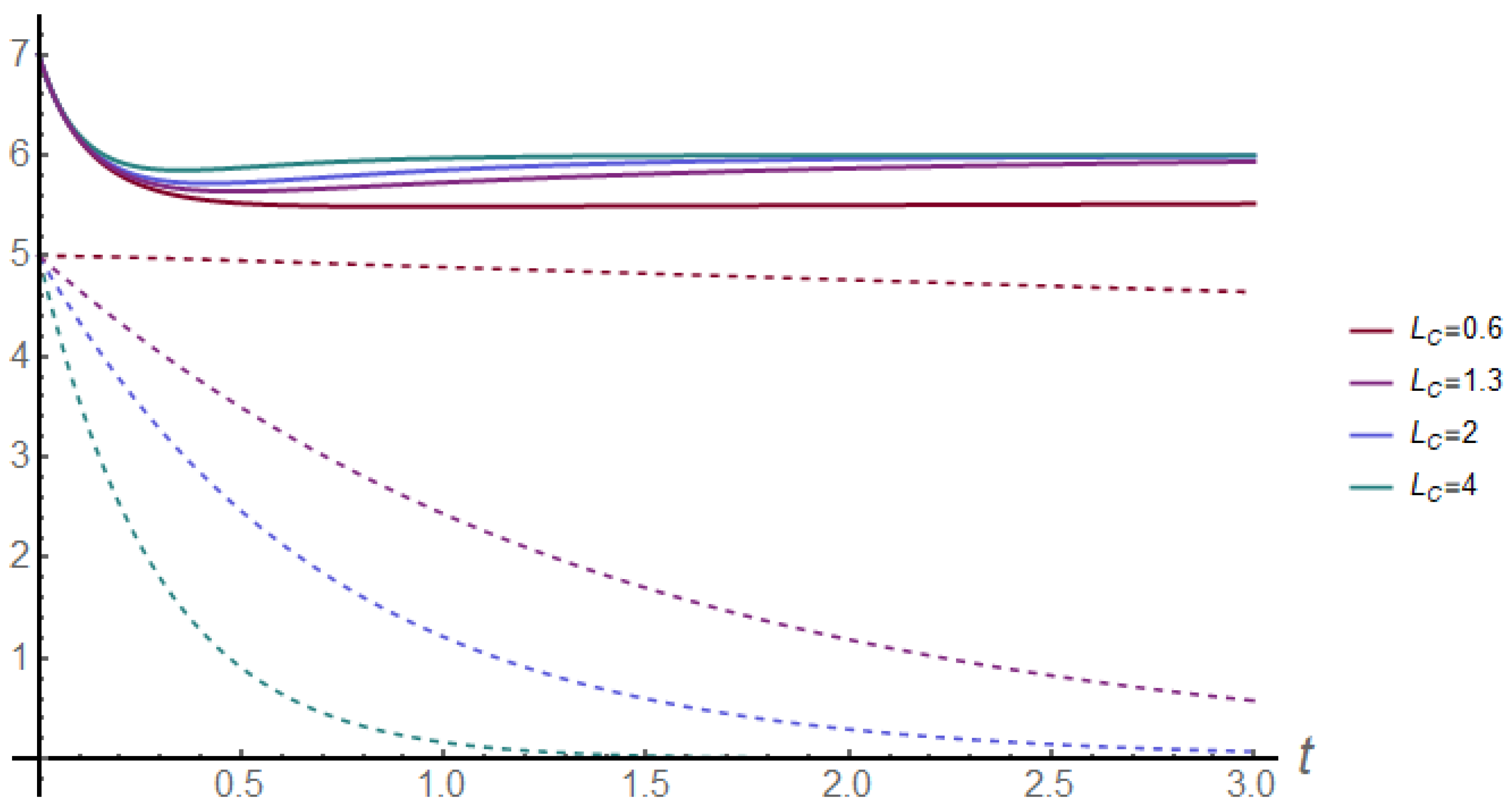
Let us observe that, if $L_C$ is sufficiently large, according to (ii) of Proposition 1, $E_1$ is stable. Therefore, ${\displaystyle L_C^{thr}=-\gamma +\frac{Kb}{K+\sigma }}$ can be seen as a threshold value above which the crime-free equilibrium is stable. Figure 1 highlights the behavior of $N_P$ (solid lines) and $C_P$ (dashed lines) as a function of time for different values of the measure of the enforcement law $L_C.$ Here, model parameters are as in

Table 1. Fixed values for some model parameters in numerical simulations.

Parameters	$\mathit{\mu }$	K	$\mathit{\sigma }$	a	$\mathit{\gamma }$	b	${\mathit{L}}_{\mathit{C}}$
Values	8	6	1	0.9	0.23	0.95	0.46

, and $E_1\equiv (6,0)$, and $L_C^{thr}=0.58$.

From this point on, we consider the internal equilibrium $E^{\ast }.$ Evaluated for $E^{\ast }$, (22) becomes

$${\displaystyle q_{E^{\ast }}=-\mu \frac{Kb-(\gamma +L_C)(K+2\sigma )}{K[b-(\gamma +L_C)]}{\gamma }_{22}+\frac{\mu {\gamma }_{12}}{K}[Kb-(\gamma +L_C)(K+\sigma )]-\frac{a{\gamma }_{21}}{b}(\gamma +L_C).}$$

(25)

The following theorem holds.

Theorem 3.

Let us assume that (8) holds. Then, $E^{\ast }$, unstable in the absence of diffusion for ${\displaystyle L_C<-\gamma +\frac{Kb}{K+2\sigma }}$, is stabilized by the action of self- and cross-diffusion if and only if

$$\left\{\begin{array}{c}{\displaystyle k^2({\gamma }_{11}+{\gamma }_{22})>\mu \frac{Kb-(\gamma +L_C)(K+2\sigma )}{K[b-(\gamma +L_C)]}}\hfill \\ \\ \mathrm{\Gamma }{k}^4+q_{E^{\ast }}{k}^2+I_2^0\left(E^{\ast }\right)>0\hfill \end{array}\right.$$

(26)

where $q_{E^{\ast }}$ is given by (25).

Remark 6.

Since $I_2^0\left(E^{\ast }\right)>0$, then $q_{E^{\ast }}>0$ is a sufficient condition ensuring that (26)₂ is satisfied.

In view of Remark 6, denoted by

$$A_1=\frac{\mu }{K}[Kb-(\gamma +L_C)(K+\sigma )]\frac{{\gamma }_{12}}{{\gamma }_{22}}-\frac{a}{b}(\gamma +L_C)\frac{{\gamma }_{21}}{{\gamma }_{22}},B_1=k^2\frac{({\gamma }_{11}+{\gamma }_{22})}{{\gamma }_{22}},$$

(27)

the following theorem holds.

Theorem 4.

Let us assume that (8) holds. Then, if ${\displaystyle L_C<-\gamma +\frac{Kb}{K+2\sigma },}$ a sufficient condition guaranteeing that $E^{\ast }$, unstable in the absence of diffusion, is stabilized by the action of self- and cross-diffusion is given by

$${\displaystyle \mu \frac{Kb-(\gamma +L_C)(K+2\sigma )}{K[b-(\gamma +L_C)]}<min\{A_1,B_1\},}$$

(28)

with $A_1,B_1$ defined as in (27).

Now we are looking for conditions ensuring that the coexistence equilibrium $E^{\ast }$, stable when the diffusion is absent, becomes unstable when the effect of diffusion is considered.

We observe that the self-diffusion alone (${\gamma }_{12}={\gamma }_{21}=0$) does not lead to the occurrence of Turing instability.

Since $I_1^0\left(E^{\ast }\right)<0$ implies $I_1\left(E^{\ast }\right)<0$ for all k, Turing instability may occur only if $I_2\left(E^{\ast }\right)<0$ for mode $k\ne 0$. A necessary condition for the occurrence of Turing instability is $q_{E^{\ast }}<0$.

The condition for the marginal stability at $k^2=k_{cr}^2$ is ${\displaystyle min\left(I_2\left(k_{cr}^2\right)\right)=0.}$ Such a minimum value of $I_2\left(k^2\right)$ is reached at ${\displaystyle k_{cr}^2=-\frac{q_{E^{\ast }}}{2\mathrm{\Gamma }}}$.

In addition, $I_2\left(k_{cr}^2\right)<0$ gives $q_{E^{\ast }}^2-4\mathrm{\Gamma }{I}_2^0\left(E^{\ast }\right)>0.$ Then, the conditions for the occurrence of cross-diffusion-driven instability for $E^{\ast }$ can be summarized in the following main theorem.

Theorem 5.

Let us assume that (8) and (3) hold. The conditions for cross-diffusion-driven instability of the homogeneous steady state $E^{\ast }$ are given by

$$\left\{\begin{array}{c}{a}_{11}<0,a_{12}{\gamma }_{21}+a_{21}{\gamma }_{12}-a_{11}{\gamma }_{22}<0,\hfill \\ \\ {(a_{12}{\gamma }_{21}+a_{21}{\gamma }_{12}-a_{11}{\gamma }_{22})}^2>-4({\gamma }_{11}{\gamma }_{22}-{\gamma }_{12}{\gamma }_{21})a_{12}{a}_{21}.\hfill \end{array}\right.$$

(29)

The above inequalities (29) define a region where the coexistence equilibrium E* is unstable. When choosing ${\gamma }_{12}$ as bifurcation parameter and ${\gamma }_{12}={\gamma }_{12}^{cr}$ as the Turing threshold, bifurcation happens at the critical value

$${\displaystyle {\gamma }_{12}^{cr}=\frac{a_{12}{\gamma }_{21}+a_{11}{\gamma }_{22}+2\sqrt{a_{12}{\gamma }_{22}(a_{11}{\gamma }_{21}-a_{21}{\gamma }_{11})}}{a_{21}}}$$

(30)

corresponding with the critical wavenumber

$${\displaystyle k_{cr}^2=\sqrt{-\frac{a_{12}{a}_{21}}{{\gamma }_{11}{\gamma }_{22}-{\gamma }_{12}{\gamma }_{21}}}\ne 0.}$$

(31)

For ${\gamma }_{12}>{\gamma }_{12}^{cr}$, the unstable wavenumbers stay in between the roots $k_{-}^2,k_{+}^2$, the roots of $I_2\left(k^2\right)=0$. We conclude this section by highlighting the existence of the Turing–Hopf bifurcation at the point of intersection of the Hopf and Turing bifurcation curves. In the vicinity of this point, it is possible to observe both the formation of inhomogeneous stationary patterns generated by Turing instabilities and the occurrence of homogeneous oscillations generated by the Hopf bifurcation. This coexistence can lead to the eventual appearance of an interesting class of spatio-temporal behaviors. When the kinetics of system (1) exhibits a Hopf bifurcation ($0<I_1^0\left(E^{\ast }\right)<<1$), highlighting a limit cycle, if $I_1\left(E^{\ast }\right)<0,$$I_2\left(E^{\ast }\right)<0$, then weak Turing–Hopf instabilities appear. These instabilities are represented as slight oscillations which have the frequency of the cycle solution superimposed on a predominantly inhomogeneous pattern. It is observed that these oscillations increase with increasing amplitude of the limit cycle, that is, with increasing $I_1^0\left(E^{\ast }\right).$

4. Numerical Simulations

In this paper, an analytical study of the interaction of two spatially distributed populations, the criminally minded population and the non-criminally minded one, has been performed. In order to show the theoretical results and highlight the effect of diffusion on the behavior of populations, in this section, we provide some numerical simulations. First, we fix values to ${\gamma }_{11},{\gamma }_{22}$ and ${\gamma }_{21}.$ We choose ${\gamma }_{12}$ as a bifurcation parameter. According to Theorem 5, from (30), we obtain ${\gamma }_{12}^{cr}$ as the minimum value for Turing instability to occur. 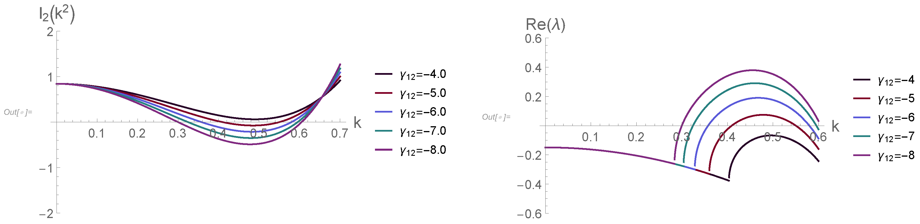Figure 2 depicts the plots of $I_2\left(k^2\right)$ for different values of the bifurcating parameter ${\gamma }_{12}$. Specifically, we have chosen ${\gamma }_{11}=0.8,{\gamma }_{22}=2,{\gamma }_{21}=3$ and other parameter values as shown in Table 1. In this case, ${\gamma }_{12}^{cr}\approx -4.445$. As we can see, for ${\gamma }_{12}=-4.0>{\gamma }_{12}^{cr}$, the graph shows that the curve does not intersect the horizontal axis, and, consequently, there are no unstable modes. As ${\gamma }_{12}$ decreases, the interval of unstable modes increases as well. Analogously, as the bifurcation parameter decreases, the real part of the corresponding eigenvalue $\lambda \left(k\right)$ becomes positive (right panel of Figure 2).

We have solved system (2) in the domain $\mathrm{\Omega }=[0,40]\times [0,40]$ with initial conditions (4) and homogeneous Neumann boundary conditions (5). The initial data have been chosen as a random perturbation of the coexistence equilibrium. For the spatial discretization, we use finite differences with step $h=0.2$. For the time discretization, we use the explicit Euler’s method, with the time step varying from ${10}^{-4}$ to ${10}^{-5}$ depending on the parameters. We have considered the model parameters shown in Table 1. 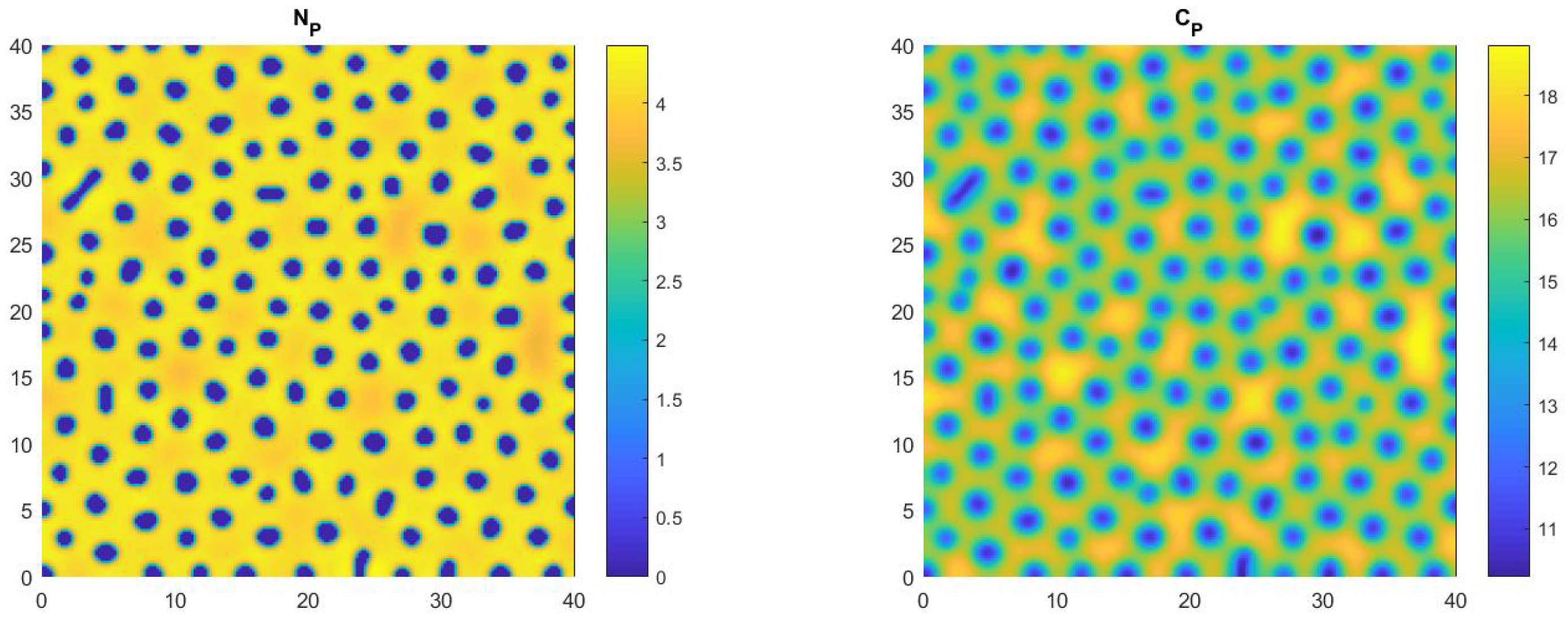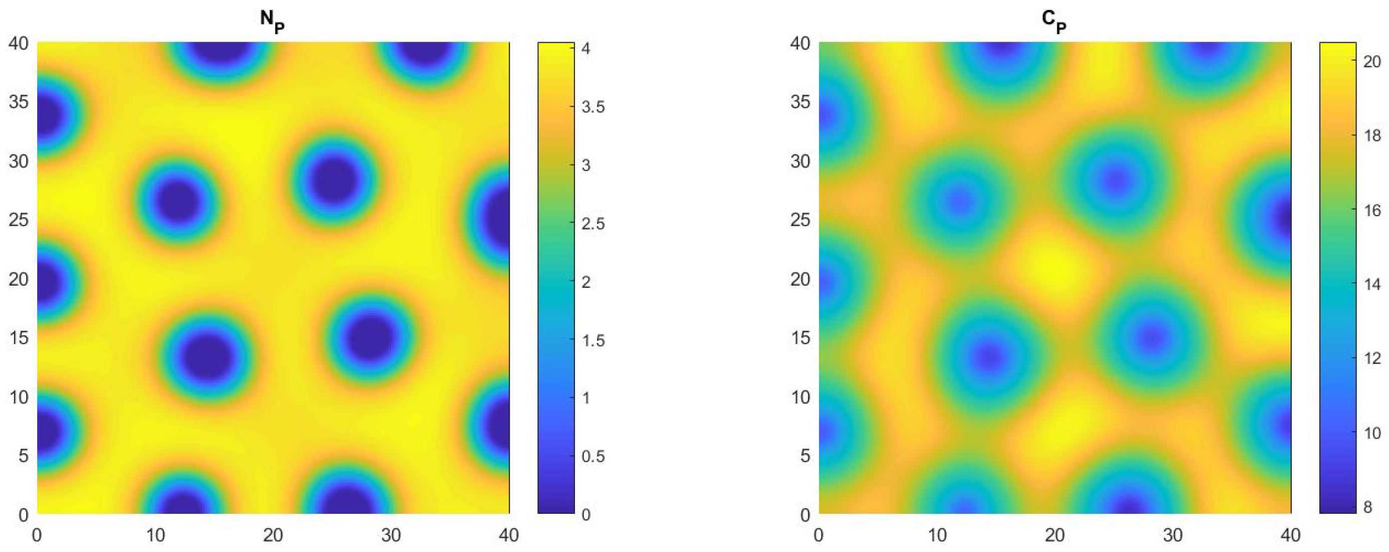Figure 3, Figure 4, Figure 5 and Figure 6 show snapshots of patterns which depict different possible scenarios. In every pattern, the blue color represents the low density of the population, and the yellow color represents the high density of that population. By various numerical simulations, we have observed that both populations are distributed predominantly over the entire domain, with some very low-density patches, generating predominantly spot patterns. Socially, yellow spots on a blue background (see Figure 6) represent that the criminally minded population exists in isolated regions with high density, motivated, for example, by the need to cooperate with other criminal individuals. 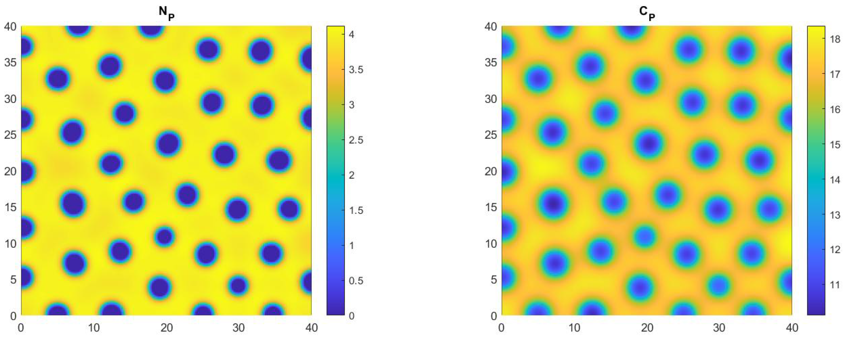For Figure 3 and Figure 4, we have chosen negative cross-diffusion coefficients (${\gamma }_{12}=-0.8,{\gamma }_{21}=-0.1$ and ${\gamma }_{12}=-3,{\gamma }_{21}=-1$, respectively) and other diffusion coefficients (${\gamma }_{11}=0.3,{\gamma }_{22}=0.5$ and ${\gamma }_{11}=2,{\gamma }_{22}=2$, respectively). In such figures, as the spread of individuals from both populations increases, it is observed that the disposition of the spots becomes more regular. For Figure 5, we have chosen a negative cross-diffusion coefficient ${\gamma }_{12}=-5$ and other diffusion coefficients as follows: ${\gamma }_{11}=0.8,{\gamma }_{22}=2,{\gamma }_{21}=3,$ satisfying the conditions of the Turing instability region. For Figure 6, we have chosen positive cross-diffusion coefficients ${\gamma }_{12}=1,{\gamma }_{21}=3.9$ and other diffusion coefficients as follows: ${\gamma }_{11}=2,{\gamma }_{22}=2,$ satisfying the conditions of the Turing instability region. This choice of positive ${\gamma }_{12}$ (${\gamma }_{21}$) depicts the social scenario in which the non-criminally minded population (criminally minded population) gravitates towards regions with a lower concentration of criminally minded individuals (non-criminally minded population).

It is interesting to note that, in this last case (Figure 6), it is possible to observe a duality, wherein non-criminally minded individuals live in regions without criminally minded individuals and vice versa. Instead, in the other cases (Figure 3, Figure 4 and Figure 5), the patterns share the property wherein both criminally minded and non-criminally minded individuals coexist in the same region.

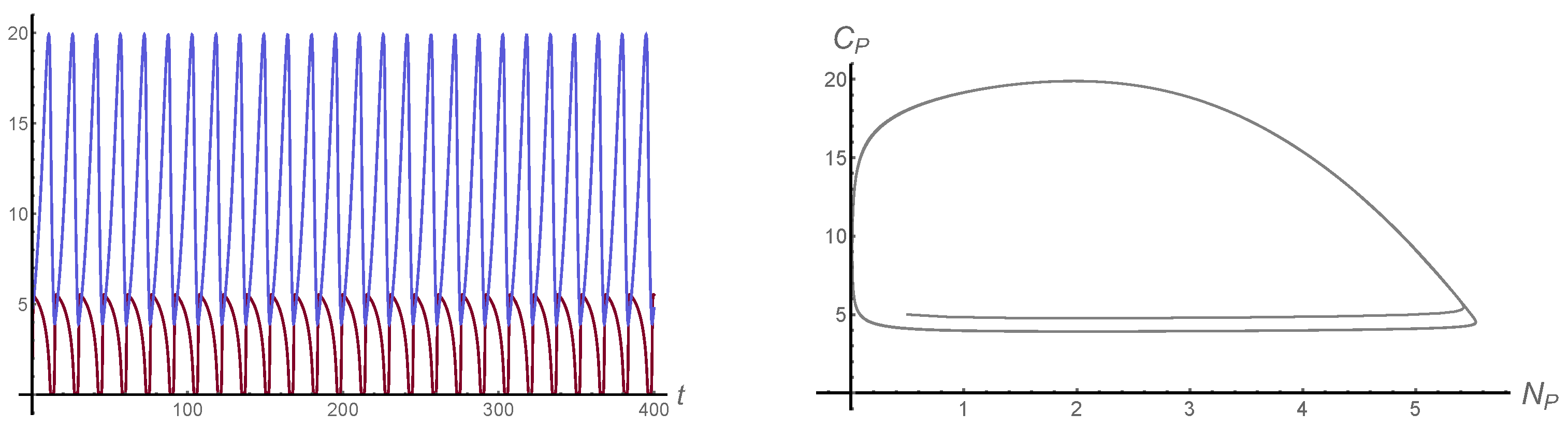
We end this section by considering the region around the Turing–Hopf bifurcation. We perform simulations for a parameter set of interest. When we choose $L_C=0.4$ and set other parameters as shown in Table 1, (19) is satisfied, and the coexistence equilibrium $E^{\ast }=(1.97,17.73)$ is oscillatory, exhibiting limit cycles. In Figure 7 (right panel), a plot of the limit cycle in the phase plane (with initial conditions $(N_P\left(0\right),C_P\left(0\right))=(0.5,5)$) is shown. The left panel of the same figure shows the time evolution of both criminally minded and non-criminally minded populations.

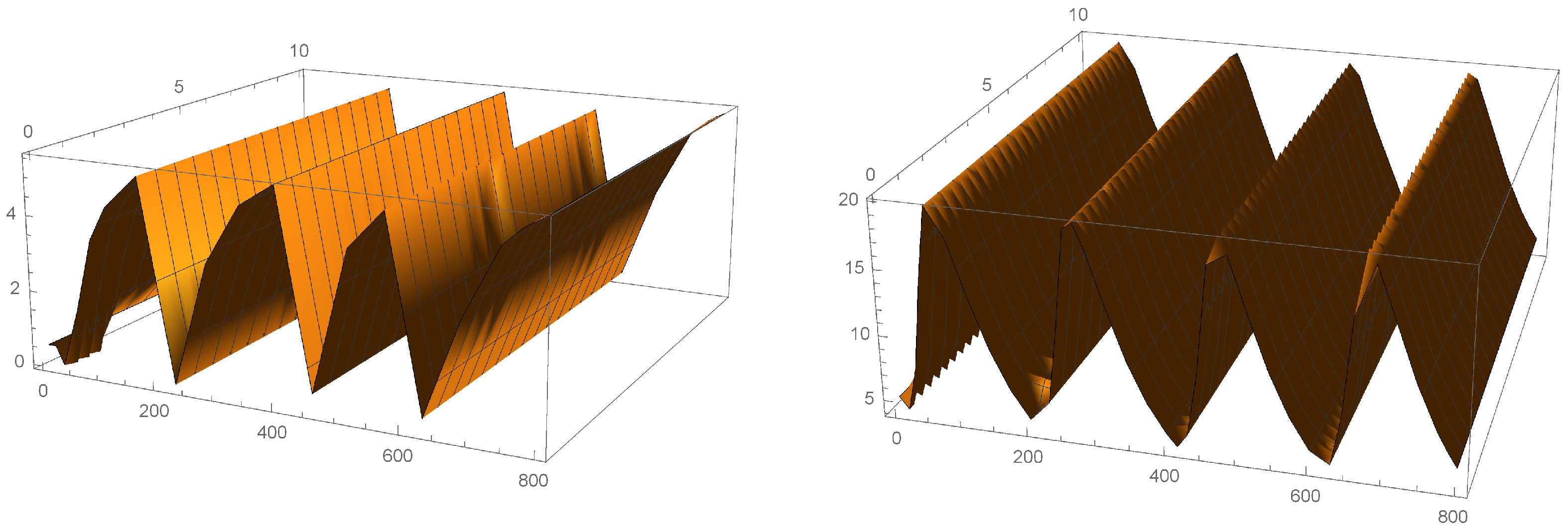
Keeping the same parameter values as in Figure 7, we simulate the corresponding diffusive model (2). For the sake of completeness, it should be clarified that both 1D and 2D experiments have been performed, but we prefer to show only the results for the 1D setting with the intention of highlighting the complete trajectories of both populations since the graphs for the 2D setting could only be obtained at certain fixed instants of time. Various numerical experiments with different sets of diffusion coefficients (satisfying the Turing conditions) allowed us to observe that the same type of instability observed in the ODE model persists, and the system still shows an oscillatory behavior. Figure 8 reports the trajectories for the non-criminally minded and criminally minded populations up to $T=800,$ with ${\gamma }_{11}=0.5,{\gamma }_{22}=2,{\gamma }_{12}=0.4,{\gamma }_{21}=-1.5.$ As evidenced by the numerical simulations conducted, spatial diffusion can deeply influence the behavior of social dynamics.

5. Conclusions

In this paper, a generalized crime model is introduced to describe the interaction between non-criminally minded and criminally minded populations. In particular, random movement of both populations is allowed. The more general case in which the diffusion of one population depends on the movement of the other population is analyzed (cross-diffusion system). This study shows the importance of considering population movement and spatial heterogeneity (which is nowadays well known and recognized in many fields) in the analysis of social interactions. In some cases, the explicit introduction of spatial diffusion can modify the forecasts of the non-spatial counterpart model. A linear instability analysis of the coexistence equilibrium (when it exists) is performed. In particular, conditions guaranteeing cross-diffusion-induced instability have been determined. Numerical simulations performed on the obtained results are shown. In particular, by varying the values of the diffusion coefficients, Turing patterns emerge, representing a spatial redistribution of the population in the environment. Destabilizing mechanisms of the coexistence equilibrium and some investigations for the possible oscillatory phenomena are applied. Extensive numerical simulations highlighting such interesting dynamics are performed.