
Application of Dandelion Optimization Algorithm in Pattern Synthesis of Linear Antenna Arrays
Abstract
:1. Introduction
2. Dandelion Optimization Algorithm
2.1. Inspiration
2.2. Mathematical Model
2.2.1. Initialization
2.2.2. Rising Process
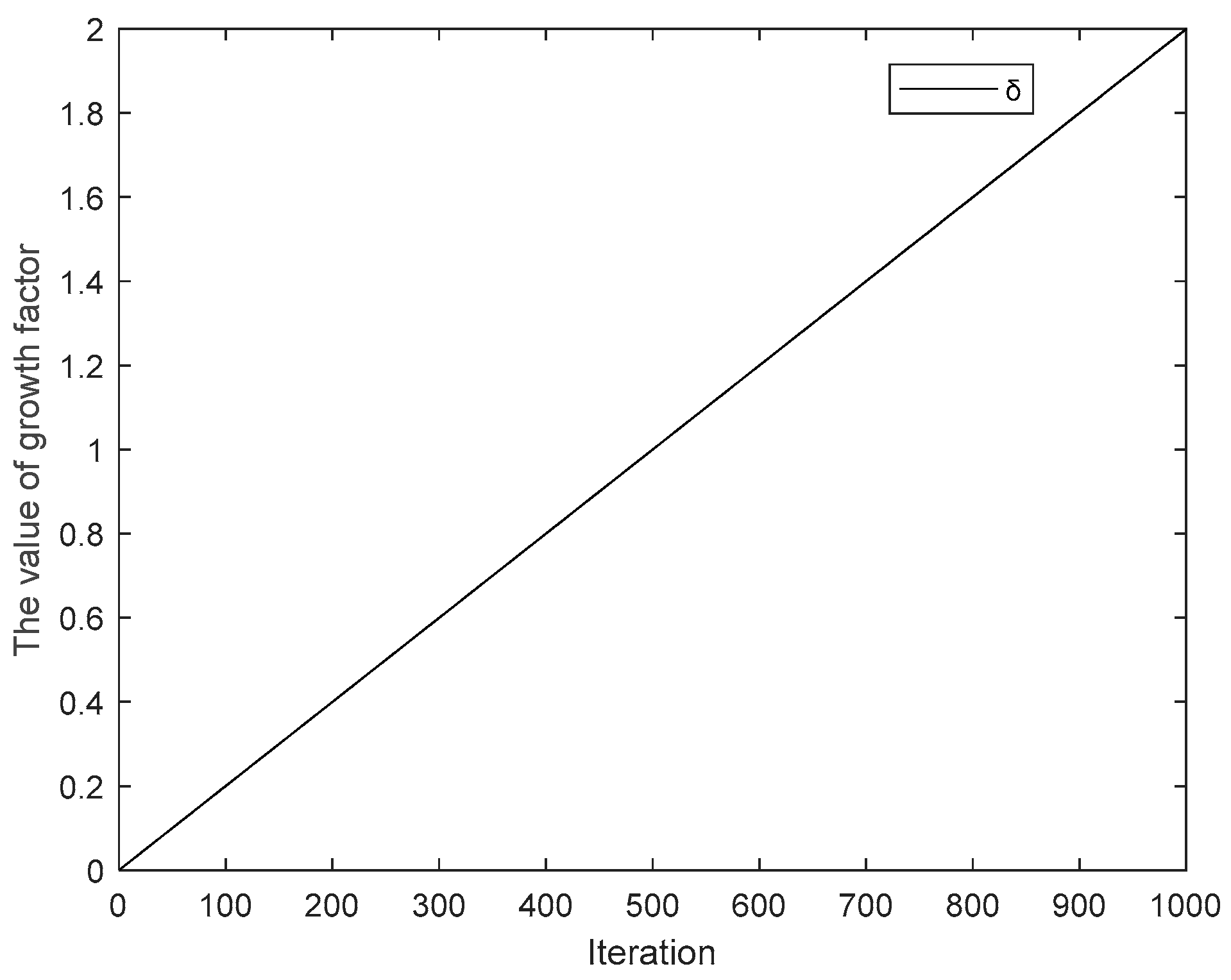
2.2.3. Descending Process
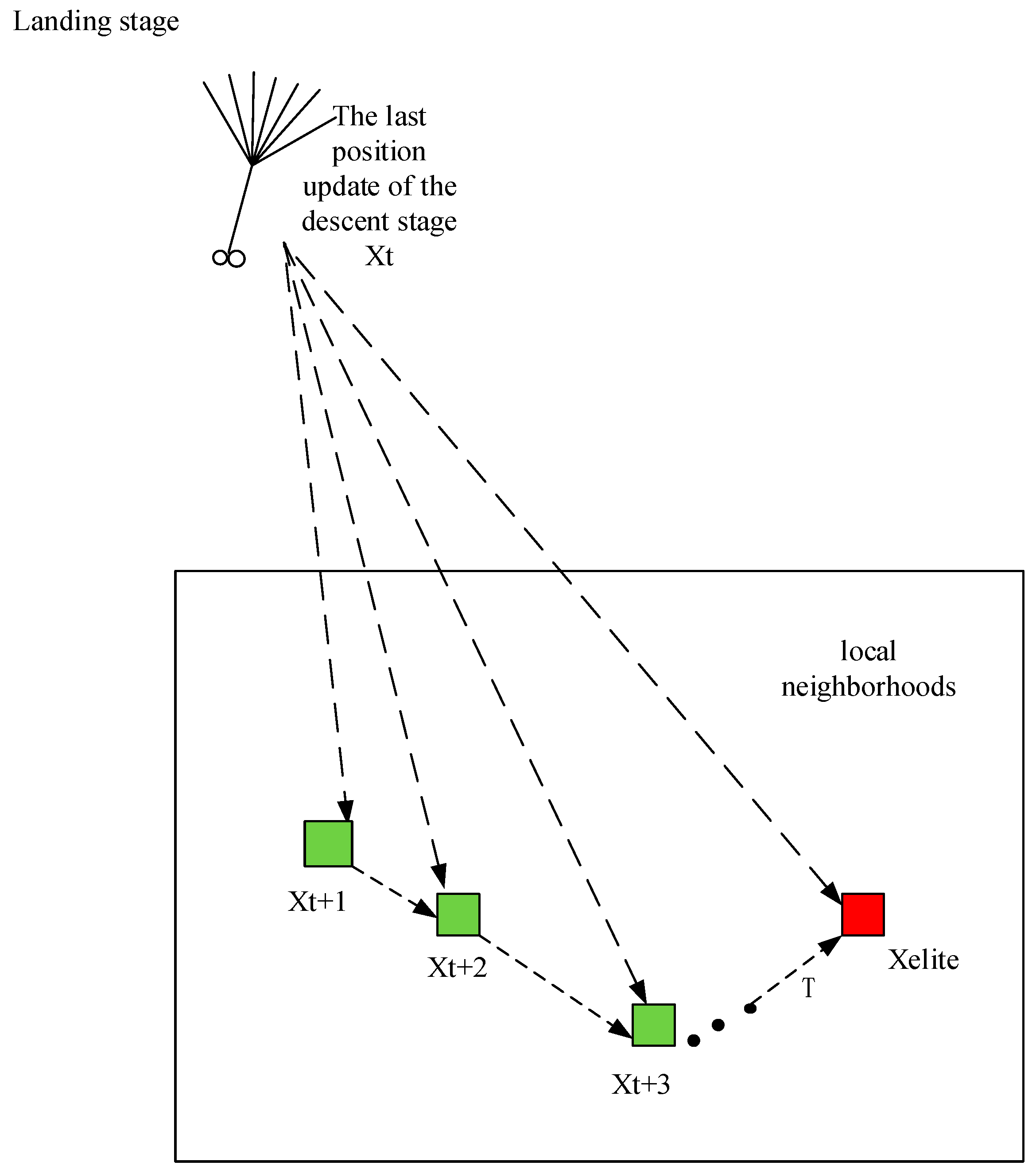
2.2.4. Landing Process
2.3. Time Complexity
3. Linear Antenna Array Synthesis
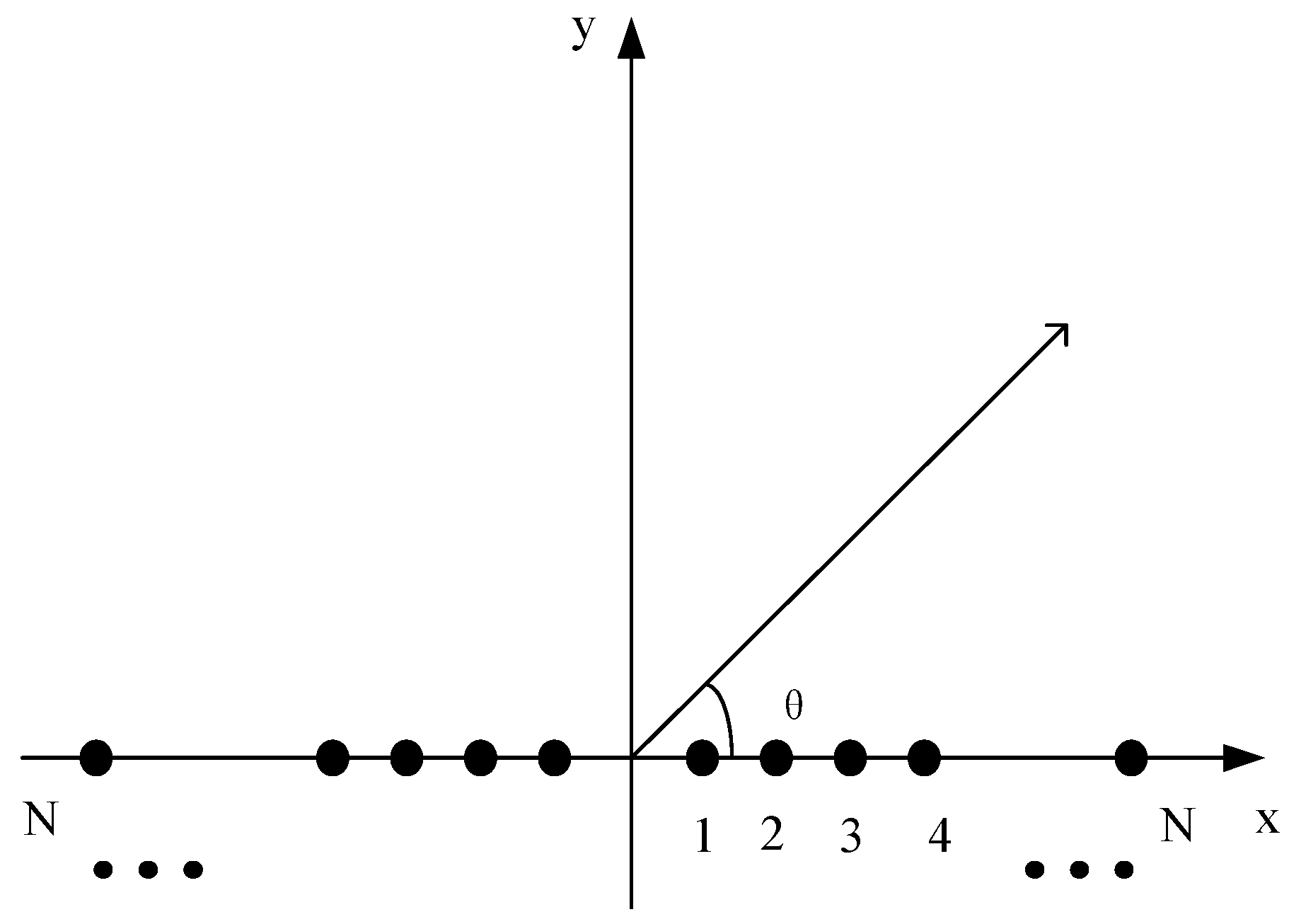
3.1. Geometric Illustration of Linear Antenna Array
3.2. Antenna Current Optimization
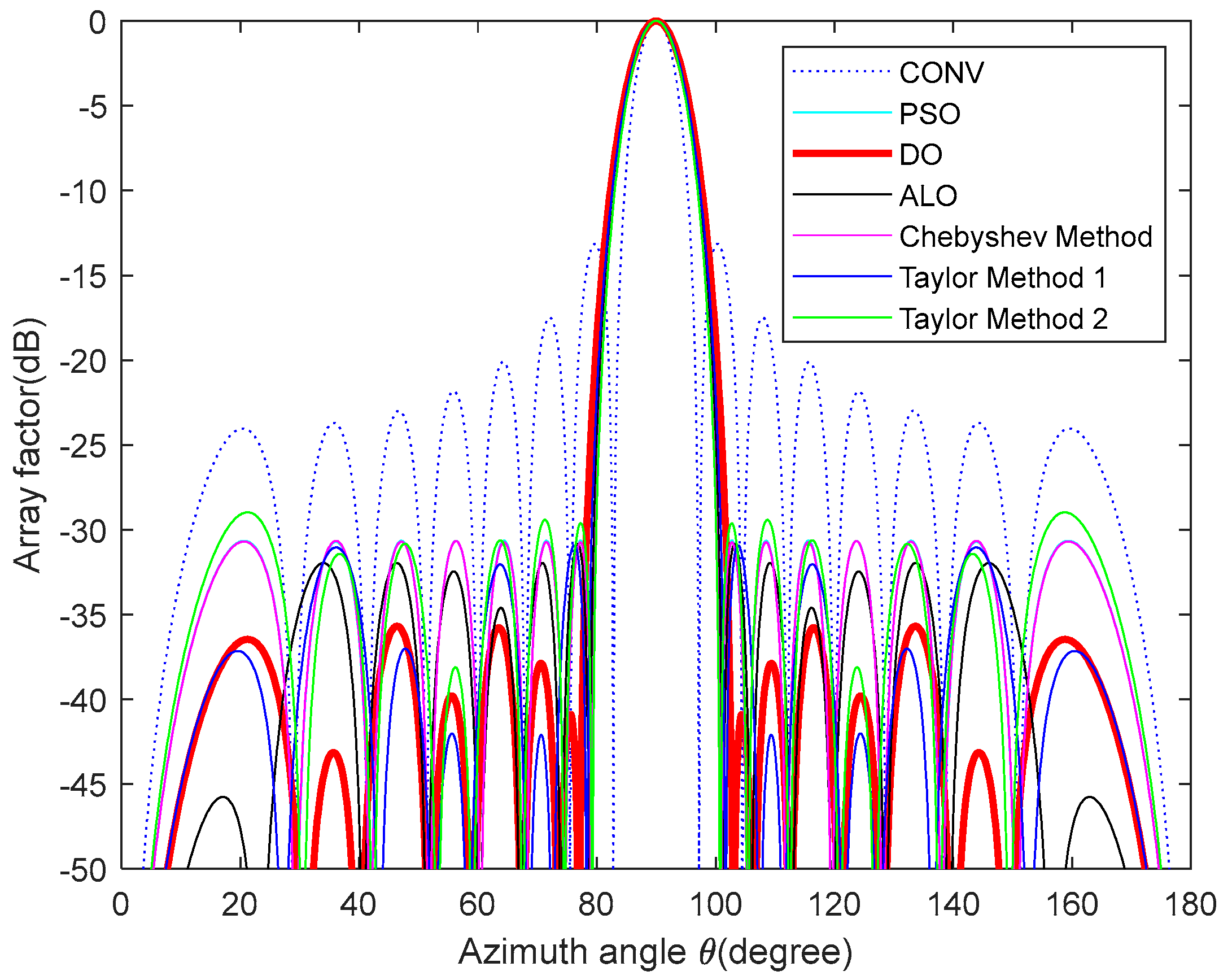
3.2.1. Minimizing Peak SLL
3.2.2. Minimizing Peak SLL and Forming Deep Nulls
3.3. Antenna Position Optimization
3.3.1. Minimizing Peak SLL
3.3.2. Minimizing Peak SLL and Forming Deep Nulls
4. Conclusions
Author Contributions
Funding
Data Availability Statement
Conflicts of Interest
References
- Yang, Y.H.; Sun, B.H.; Guo, J.L. A low-cost, single-layer, dual circularly polarized antenna for millimeter-wave applications. IEEE Antennas Wirel. Propag. Lett. 2019, 18, 651–655. [Google Scholar] [CrossRef]
- Bilgic, M.M.; Yegin, K. Modified annular ring antenna for GPS and SDARS automotive applications. IEEE Antennas Wirel. Propag. Lett. 2015, 15, 1442–1445. [Google Scholar] [CrossRef]
- Mobashsher, A.T.; Pretorius, A.J.; Abbosh, A.M. Low-profile vertical polarized slotted antenna for on-road RFID-enabled intelligent parking. IEEE Trans. Antennas Propag. 2019, 68, 527–532. [Google Scholar] [CrossRef]
- Liu, J.L.; Su, T.; Liu, Z.X. High-gain grating antenna with surface wave launcher array. IEEE Antennas Wirel. Propag. Lett. 2018, 17, 706–709. [Google Scholar] [CrossRef]
- Huang, H.; Gao, S.; Lin, S.; Ge, L. A wideband water patch antenna with polarization diversity. IEEE Antennas Wirel. Propag. Lett. 2020, 19, 1113–1117. [Google Scholar] [CrossRef]
- Pietrenko-Dabrowska, A.; Koziel, S.; Ullah, U. Reduced-cost two-level surrogate antenna modeling using domain confinement and response features. Sci. Rep. 2022, 12, 4667. [Google Scholar] [CrossRef] [PubMed]
- Pietrenko-Dabrowska, A.; Koziel, S. On EM-driven size reduction of antenna structures with explicit constraint handling. IEEE Access 2021, 9, 165766–165772. [Google Scholar] [CrossRef]
- Koziel, S.; Pietrenko-Dabrowska, A. Design-oriented modeling of antenna structures by means of two-level kriging with explicit dimensionality reduction. AEU-Int. J. Electron. Commun. 2020, 127, 153466. [Google Scholar] [CrossRef]
- Sarker, M.A.; Hossain, M.S.; Masud, M.S. Robust beamforming synthesis technique for low side lobe level using taylor excited antenna array. In Proceedings of the 2016 2nd International Conference on Electrical, Computer & Telecommunication Engineering (ICECTE), Rajshahi, Bangladesh, 8–10 December 2016; IEEE: New York, NY, USA, 2016; pp. 1–4. [Google Scholar]
- Dorigo, M.; Gambardella, L.M. Ant colony system: A cooperative learning approach to the traveling salesman problem. IEEE Trans. Evol. Comput. 1997, 1, 53–66. [Google Scholar] [CrossRef]
- Kennedy, J.; Eberhart, R. Particle swarm optimization. In Proceedings of the ICNN’95-International Conference on Neural Networks, Perth, WA, Australia, 27 November–1 December 1995; IEEE: New York, NY, USA, 1995; Volume 4, pp. 1942–1948. [Google Scholar]
- Davis, L.D. Handbook of Genetic Algorithms; Van Nostrand Reinhold: New York, NY, USA; Santa Fe, NM, USA, 1991. [Google Scholar]
- Storn, R.; Price, K. Differential evolution-a simple and efficient heuristic for global optimization over continuous spaces. J. Glob. Optim. 1997, 11, 341. [Google Scholar] [CrossRef]
- Goudos, S.K.; Siakavara, K.; Sahalos, J.N. Novel spiral antenna design using artificial bee colony optimization for UHF RFID applications. IEEE Antennas Wirel. Propag. Lett. 2014, 13, 528–531. [Google Scholar] [CrossRef]
- Quevedo-Teruel, O.; Rajo-Iglesias, E. Ant colony optimization in thinned array synthesis with minimum sidelobe level. IEEE Antennas Wirel. Propag. Lett. 2006, 5, 349–352. [Google Scholar] [CrossRef]
- Al-Azza, A.A.; Al-Jodah, A.A.; Harackiewicz, F.J. Spider monkey optimization: A novel technique for antenna optimization. IEEE Antennas Wirel. Propag. Lett. 2015, 15, 1016–1019. [Google Scholar] [CrossRef]
- Goudos, S.K.; Siakavara, K.; Samaras, T.; Vafiadis, E.E.; Sahalos, J.N. Self-adaptive differential evolution applied to real-valued antenna and microwave design problems. IEEE Trans. Antennas Propag. 2011, 59, 1286–1298. [Google Scholar] [CrossRef]
- Ram, G.; Mandal, D.; Kar, R.; Ghoshal, S.P. Cat swarm optimization as applied to time-modulated concentric circular antenna array: Analysis and comparison with other stochastic optimization methods. IEEE Trans. Antennas Propag. 2015, 63, 4180–4183. [Google Scholar] [CrossRef]
- Darvish, A.; Ebrahimzadeh, A. Improved fruit-fly optimization algorithm and its applications in antenna arrays synthesis. IEEE Trans. Antennas Propag. 2018, 66, 1756–1766. [Google Scholar] [CrossRef]
- Karimkashi, S.; Kishk, A.A. Invasive weed optimization and its features in electromagnetics. IEEE Trans. Antennas Propag. 2010, 58, 1269–1278. [Google Scholar] [CrossRef]
- Wolpert, D.H.; Macready, W.G. No free lunch theorems for optimization. IEEE Trans. Evol. Comput. 1997, 1, 67–82. [Google Scholar] [CrossRef]
- Zhao, S.; Zhang, T.; Ma, S.; Chen, M. Dandelion Optimizer: A nature-inspired metaheuristic algorithm for engineering applications. Eng. Appl. Artif. Intell. 2022, 114, 105075. [Google Scholar] [CrossRef]
- Einstein, A. Investigations on the Theory of the Brownian Movement; Courier Corporation: North Chelmsford, MA, USA, 1956. [Google Scholar]
- Mantegna, R.N. Fast, accurate algorithm for numerical simulation of Levy stable stochastic processes. Phys. Rev. E 1994, 49, 4677. [Google Scholar] [CrossRef]
- Valian, E.; Mohanna, S.; Tavakoli, S. Improved cuckoo search algorithm for global optimization. Int. J. Commun. Inf. Technol. 2011, 1, 31–44. [Google Scholar]
- Yahya, M.; Saka, M.P. Construction site layout planning using multi-objective artificial bee colony algorithm with Levy flights. Autom. Constr. 2014, 38, 14–29. [Google Scholar] [CrossRef]
- Raji, M.F.; Zhao, H.; Monday, H.N. Fast optimization of sparse antenna array using numerical Green’s function and genetic al-gorithm. Int. J. Numer. Model. Electron. Netw. Devices Fields 2020, 33, e2544. [Google Scholar] [CrossRef]
- Balanis, C.A. Microstrip antennas. Antenna Theory Anal. Des. 2005, 3, 811–882. [Google Scholar]
- Khodier, M.M.; Al-Aqeel, M. Linear and circular array optimization: A study using particle swarm intelligence. Prog. Electromagn. Res. B 2009, 15, 347–373. [Google Scholar] [CrossRef]
- Singh, U.; Kumar, H.; Kamal, T.S. Linear array synthesis using biogeography based optimization. Prog. Electromagn. Res. M 2010, 11, 25–36. [Google Scholar] [CrossRef]
- Chatterjee, S.; Chatterjee, S.; Poddar, D.R. Synthesis of linear array using Taylor distribution and Particle Swarm Optimisation. Int. J. Electron. 2015, 102, 514–528. [Google Scholar] [CrossRef]
- Saxena, P.; Kothari, A. Ant lion optimization algorithm to control side lobe level and null depths in linear antenna arrays. AEU-Int. J. Electron. Commun. 2016, 70, 1339–1349. [Google Scholar] [CrossRef]
- Singh, U.; Salgotra, R. Optimal synthesis of linear antenna arrays using modified spider monkey optimization. Arab. J. Sci. Eng. 2016, 41, 2957–2973. [Google Scholar] [CrossRef]
- Subhashini, K.R. Runner-root algorithm to control sidelobe level and null depths in linear antenna arrays. Arab. J. Sci. Eng. 2020, 45, 1513–1529. [Google Scholar] [CrossRef]
- Urvinder, S.; Salgotra, R. Synthesis of linear antenna array using flower pollination algorithm. Neural Comput. Appl. 2018, 29, 435–445. [Google Scholar]
- Hu, K.; Liu, Y.; Zhao, K. Application of chaotic colony predation algorithm in electromagnetics. Phys. Scr. 2023, 98, 105516. [Google Scholar] [CrossRef]
- Saxena, P.; Kothari, A. Optimal pattern synthesis of linear antenna array using grey wolf optimization algorithm. Int. J. Antennas Propag. 2016, 2016, 1205970. [Google Scholar] [CrossRef]
- Wang, H.; Liu, C.; Wu, H.; Li, B.; Xie, X. Optimal pattern synthesis of linear array and broadband design of whip antenna using grasshopper optimization algorithm. Int. J. Antennas Propag. 2020, 2020, 5904018. [Google Scholar] [CrossRef]
- Liang, Q.; Chen, B.; Wu, H.; Ma, C.; Li, S. A novel modified sparrow search algorithm with application in side lobe level reduction of linear antenna array. Wirel. Commun. Mob. Comput. 2021, 2021, 9915420. [Google Scholar] [CrossRef]
- Pappula, L.; Ghosh, D. Linear antenna array synthesis using cat swarm optimization. AEU-Int. J. Electron. Commun. 2014, 68, 540–549. [Google Scholar] [CrossRef]


| DO algorithm |
| Input: Population size (pop), maximum number of iterations (T), dimensionality of variables (Dim) |
| Output: Optimal dandelion (Xbest), fitness function value of optimal dandelion (fbest) |
| Initialization |
| 1: Using the DO algorithm to initialize the dandelion (Xi) population |
| 2: Calculate the fitness function value (fi) for each dandelion |
| 3: Compare the fitness values and select the dandelion (Xbest) at the optimal position corresponding to the minimum fitness value |
| 4: while (t < T) do |
| ~*Rising process*~ |
| 5: if randn < 1.5 do |
| 6: Update the adaptive parameters for adjusting step size using Equation (8) |
| 7: Update the position of dandelions using Equation (5) |
| 8: else if do |
| 9: Update the range of the search domain and adjust the step size using Equation (11) |
| 10: Update the position of dandelions using Equation (10) |
| 11: end if |
| ~*Descending process*~ |
| 12: Update the position of dandelions using Equation (13) |
| ~*Landing process*~ |
| 13: Update the position of dandelions using Equation (15) |
| 14: Arrange dandelions from good to bad according to the order of fitness values from small to large |
| 15: Update Xelite |
| 16: if f (Xelite) < f (Xbest) |
| 17: Xbest = Xelite, fbest = f (Xelite) |
| 18: end if |
| 19: end while |
| 20: return Xbest and fbest |
| Method | Optimized Current Amplitudes | Peak SLL (dB) |
|---|---|---|
| CONV (Uniform array) | 1.0000, 1.0000, 1.0000, 1.0000, 1.0000, 1.0000, 1.0000, 1.0000 | −13.15 |
| Chebyshev method [31] | 1.0000, 0.9510, 0.8600, 0.7360, 0.5930, 0.4450, 0.3060, 0.2710 | −30.70 |
| Taylor method 1 [31] | 1.0000, 0.9610, 0.9030, 0.7110, 0.5670, 0.4100, 0.2490, 0.1780 | −30.70 |
| Taylor method 2 [31] | 1.0000, 0.9860, 0.8690, 0.7330, 0.5970, 0.4900, 0.3060, 0.2650 | −29.60 |
| PSO [29] | 1.0000, 0.9521, 0.5605, 0.7372, 0.5940, 0.4465, 0.3079, 0.2724 | −30.63 |
| ALO [32] | 1.0000, 0.9344, 0.8521, 0.7044, 0.6000, 0.4000, 0.3003, 0.2002 | −30.85 |
| DO | 1.0000, 0.9600, 0.8222, 0.6789, 0.5055, 0.3513, 0.2186, 0.1367 | −35.69 |
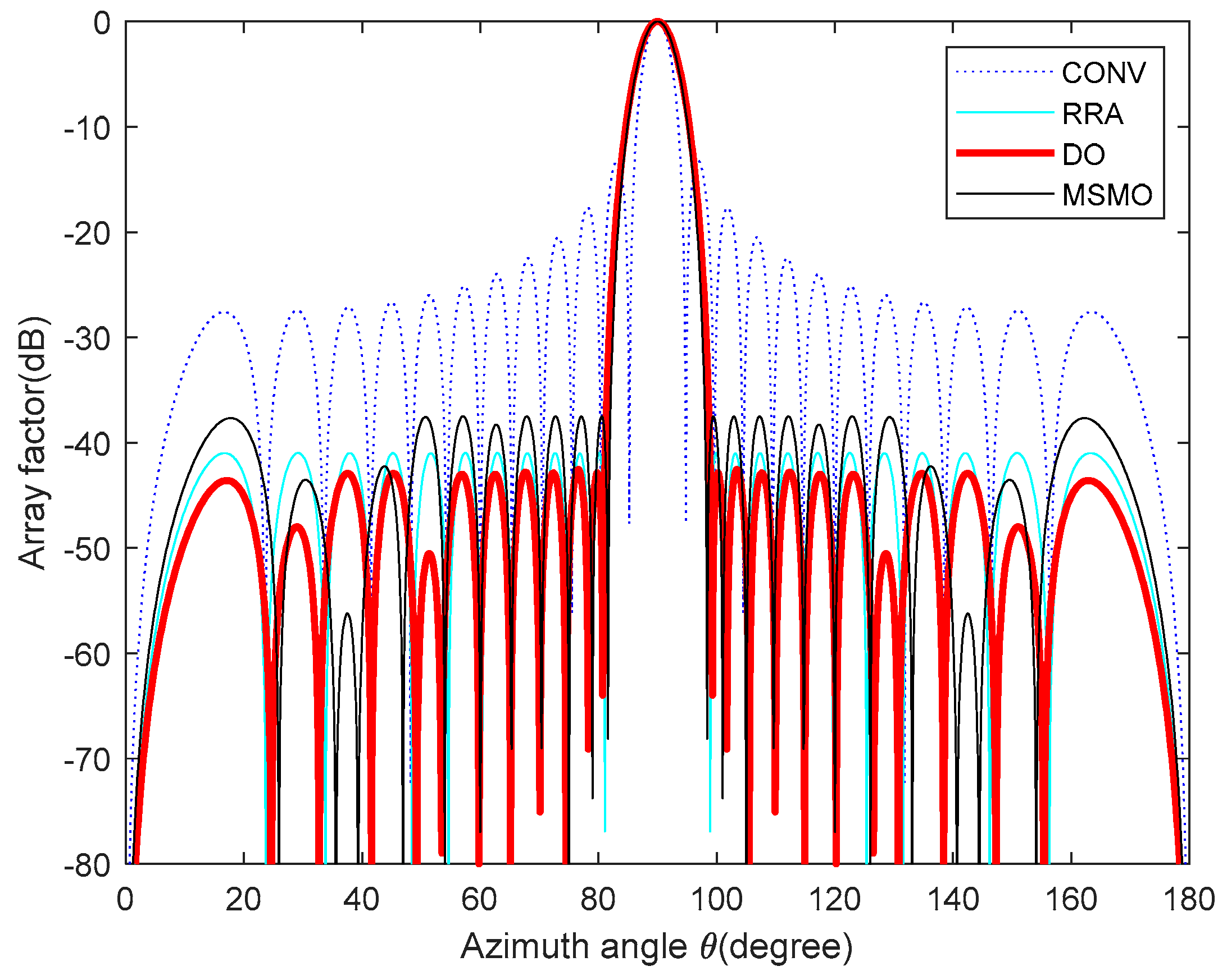
| Method | Optimized Current Amplitudes | FNBW (deg) | Peak SLL (dB) |
|---|---|---|---|
| CONV (Uniform array) | 1.0000, 1.0000, 1.0000, 1.0000, 1.0000, 1.0000 | ~ | −13.23 |
| 1.0000, 1.0000, 1.0000, 1.0000, 1.0000, 1.0000 | |||
| MSMO [33] | 1.0000, 0.9717, 0.9195, 0.8438, 0.7555, 0.6565 | 16.8 | −37.52 |
| 0.5278, 0.4534, 0.3194, 0.2430, 0.1818, 0.1296 | |||
| RRA [34] | 1.0000, 0.9706, 0.9141, 0.8344, 0.7371, 0.6287 | 17.8 | −41.08 |
| 0.5162, 0.4060, 0.3038, 0.2140, 0.1395, 0.1136 | |||
| DO | 0.8192, 0.7901, 0.7414, 0.6798, 0.5855, 0.5004 | 18.6 | −42.56 |
| 0.4069, 0.3111, 0.2287, 0.1596, 0.1018, 0.0692 |
| Array Element | 1 | 2 | 3 | 4 | 5 |
| Optimized current amplitudes | 1.0000 | 0.9933 | 0.9938 | 0.7965 | 0.6794 |
| Array Element | 6 | 7 | 8 | 9 | 10 |
| Optimized current amplitudes | 0.6581 | 0.4322 | 0.3669 | 0.2138 | 0.0956 |
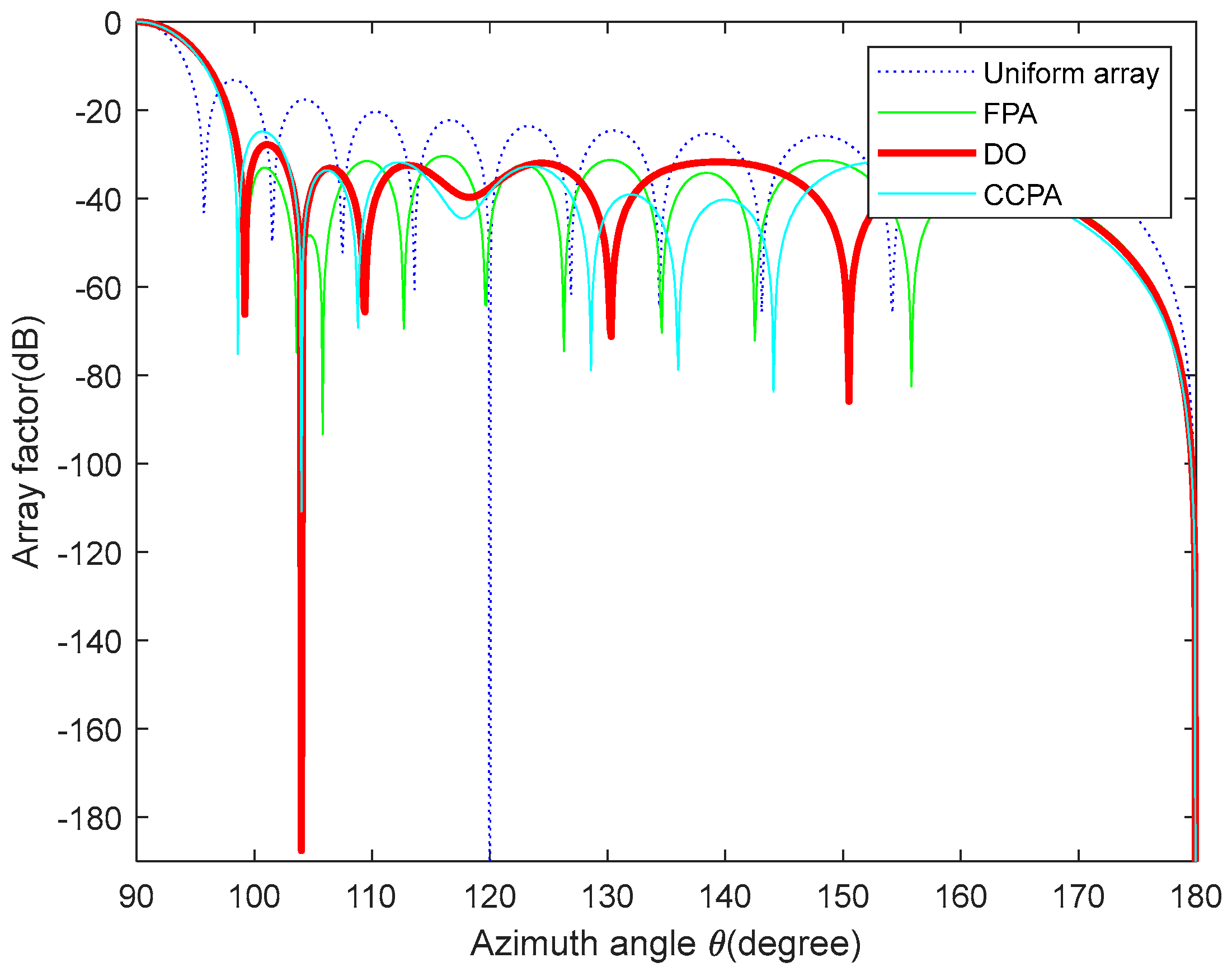
| Algorithm | Uniform Array | FPA [35] | CCPA [36] | DO |
|---|---|---|---|---|
| Peak SLL (dB) | −17.62 | −31.31 | −31.57 | −31.72 |
| Null depth (dB) | −17.69 | −120.9 | −143.3 | −187.6 |
| Method | Optimized Current Amplitudes |
|---|---|
| Uniform array | 1.0000, 1.0000, 1.0000, 1.0000, 1.0000, 1.0000, 1.0000, 1.0000, 1.0000, 1.0000 |
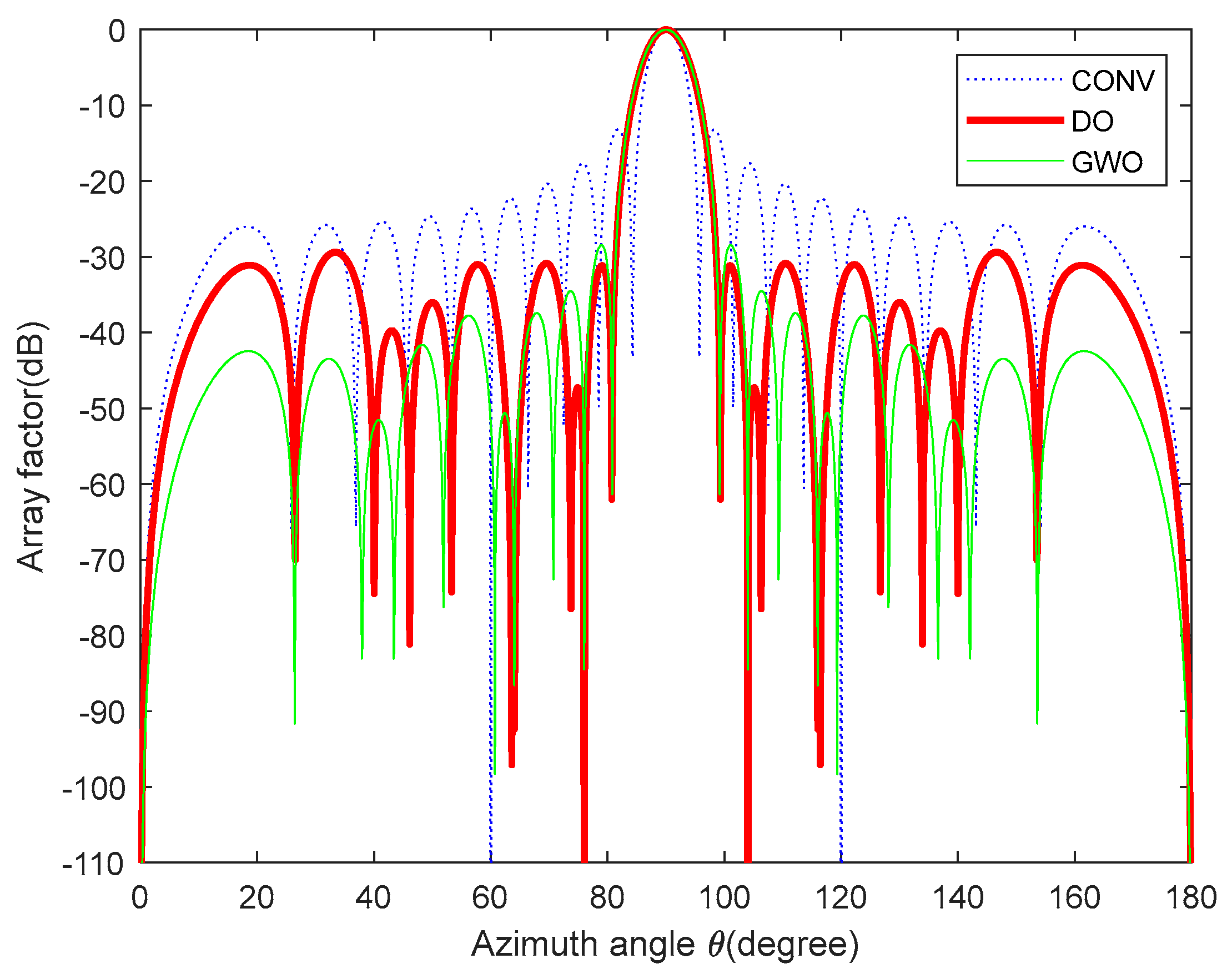
| GWO [37] | 1.0000, 0.9794, 0.9254, 0.8126, 0.7008, 0.6000, 0.4594, 0.3326, 0.2133, 0.1167 |
| DO | 0.9916, 0.9986, 1.0000, 0.8303, 0.7148, 0.6093, 0.4466, 0.3573, 0.1959, 0.2127 |
| Method | Peak SLL (dB) | Null Depth (dB) | FNBW (deg) | |||
|---|---|---|---|---|---|---|
| 64° | 76° | 104° | 116° | |||
| Uniform array | −13.19 | −22.7 | −17.7 | −17.7 | −22.7 | 11.4 |
| GWO [37] | −28.44 | −92.02 | −79.12 | −79.12 | −92.02 | 18.4 |
| DO | −29.39 | −92.37 | −131.6 | −131.6 | −92.37 | 18.6 |
| Algorithms | Peak SLL (dB) | Notch Depths (dB) | Optimized Current Amplitudes |
|---|---|---|---|
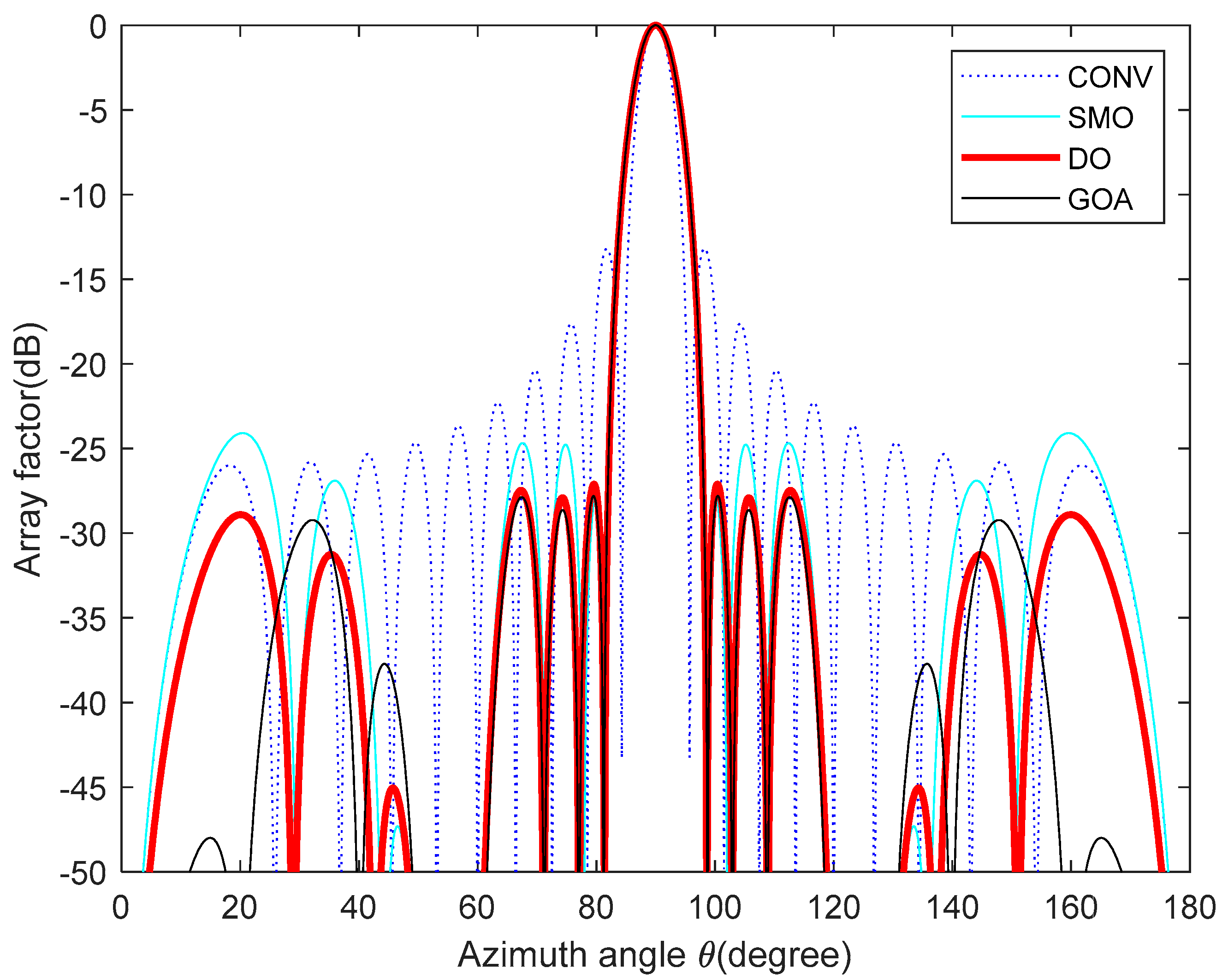
| CONV (Uniform array) | −13.2 | −23.6 | 1.000, 1.000, 1.000, 1.000, 1.000, 1.000, 1.000, 1.000, 1.000, 1.000 |
| SMO [16] | −24.1 | −56.7 | 1.000, 0.999, 1.000, 0.836, 0.643, 0.654, 0.477, 0.597, 0.258, 0.215 |
| GOA [38] | −27.7 | −61.2 | 1.000, 0.986, 0.990, 0.796, 0.736, 0.563, 0.527, 0.447, 0.243, 0.151 |
| DO | −27.1 | −63.1 | 1.000, 1.000, 0.975, 0.838, 0.687, 0.630, 0.493, 0.498, 0.233, 0.160 |
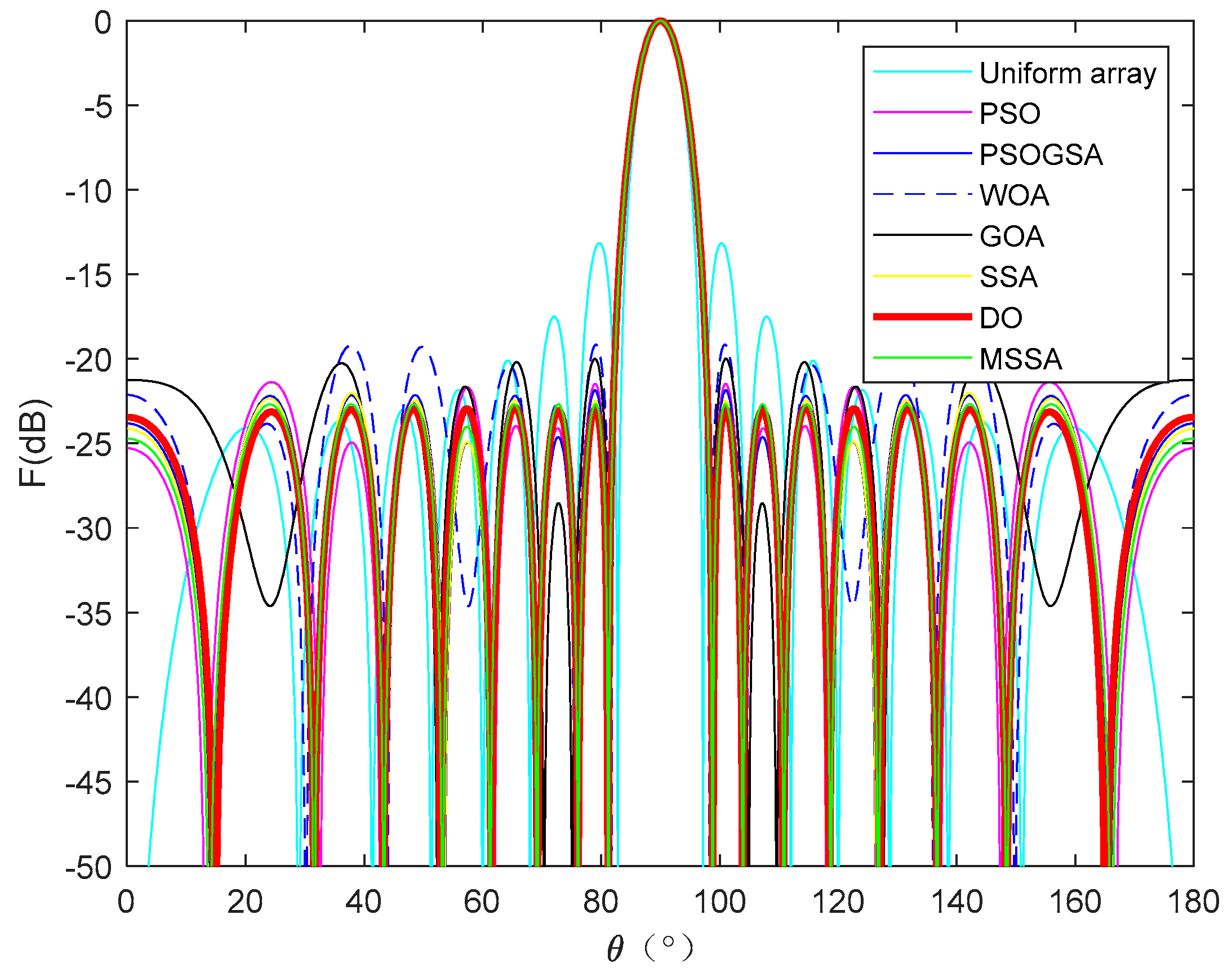
| Algorithm | Optimized Element Positions (λ) | Peak SLL (dB) |
|---|---|---|
| Uniform array | 0.2500, 0.7500, 1.2500, 1.7500, 2.2500, 2.7500, 3.2500, 3.7500 | −13.1476 |
| PSO [39] | 0.2500, 0.5311, 1.0128, 1.3930, 1.8738, 2.3329, 2.9893, 3.7500 | −21.3693 |
| PSOGSA [39] | 0.2500, 0.5495, 1.0230, 1.3560, 1.8561, 2.3358, 2.9783, 3.7500 | −21.8484 |
| WOA [39] | 0.2500, 0.6485, 1.0456, 1.3751, 1.9467, 2.4634, 3.0076, 3.7500 | −19.1546 |
| GOA [39] | 0.2500, 0.5802, 1.1274, 1.3493, 1.9119, 2.3129, 3.0208, 3.7500 | −19.9808 |
| SSA [39] | 0.2500, 0.5331, 1.0118, 1.3453, 1.8495, 2.3404, 2.9835, 3.7500 | −22.0177 |
| MSSA [39] | 0.2500, 0.5226, 1.0038, 1.3486, 1.8518, 2.3447, 2.9948, 3.7500 | −22.6768 |
| DO | 0.2500, 0.5138, 1.0025, 1.3456, 1.8454, 2.3264, 2.9886, 3.7500 | −22.8766 |
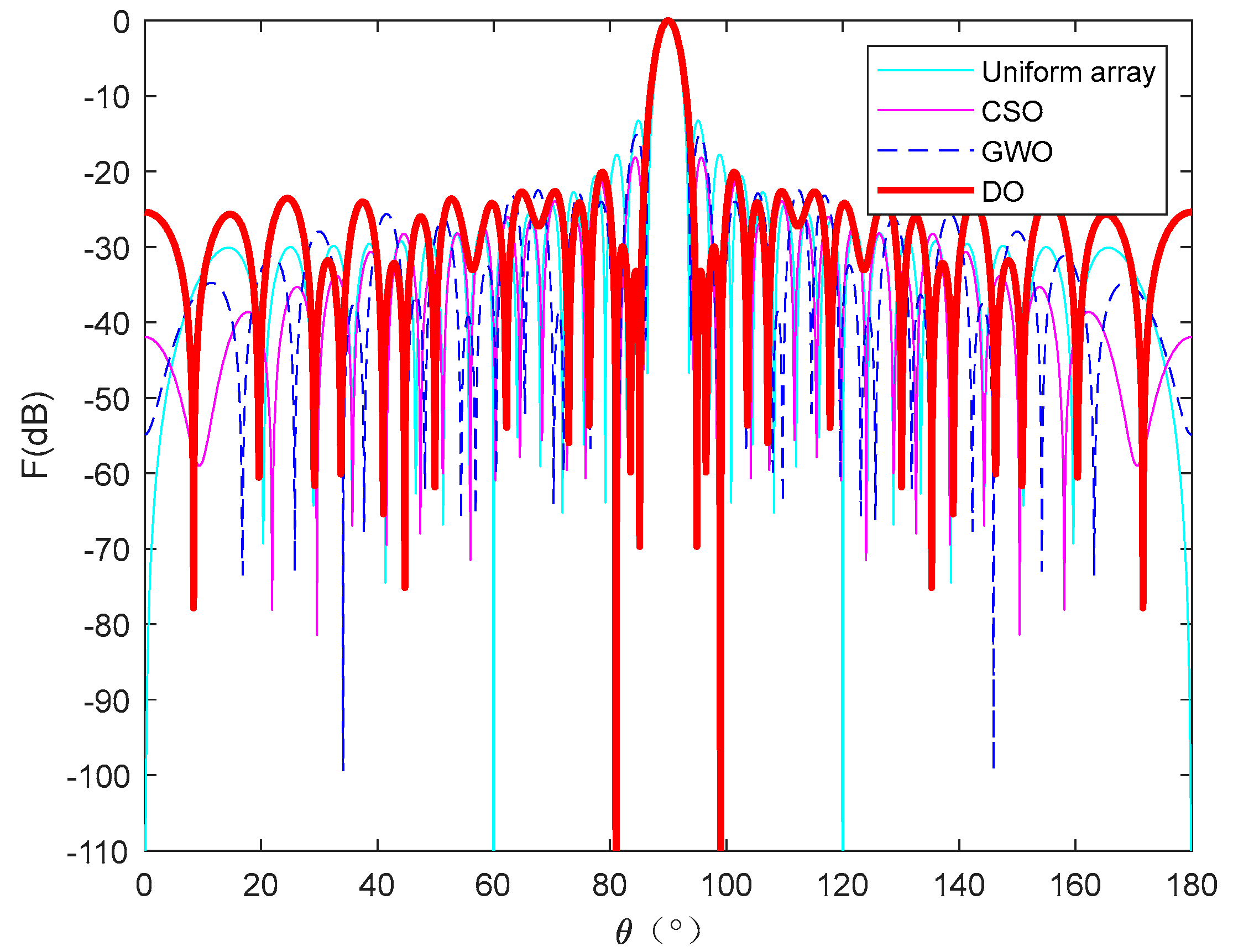
| Method | Optimized Element Positions (λ) |
|---|---|
| Uniform array | 0.2500, 0.7500, 1.2500, 1.7500, 2.2500, 2.7500, 3.2500, 3.7500 |
| 4.2500, 4.7500, 5.2500, 5.7500, 6.2500, 6.7500, 7.2500, 7.7500 | |
| CSO [40] | 0.2883, 0.6830, 1.1929, 1.5199, 1.9768, 2.3247, 2.6886, 3.1362 |
| 3.4848, 3.9538, 4.3822, 4.9252, 5.4817, 6.2091, 7.0412, 7.7500 | |
| GWO [37] | 0.194307, 0.74071, 1.249193, 1.747565, 2.241275, 2.714261, 2.999822, 3.451514 |
| 3.753935, 4.275930, 4.750000, 5.255635, 5.751775, 6.455911, 7.250000, 8.000000 | |
| DO | 0.100053, 0.736700, 0.884280, 1.379279, 1.784958, 1.815880, 2.426244, 2.800191 |
| 3.385721, 3.592616, 4.084495, 4.601558, 5.417883, 6.328078, 7.184669, 8.094933 |
Disclaimer/Publisher’s Note: The statements, opinions and data contained in all publications are solely those of the individual author(s) and contributor(s) and not of MDPI and/or the editor(s). MDPI and/or the editor(s) disclaim responsibility for any injury to people or property resulting from any ideas, methods, instructions or products referred to in the content. |
© 2024 by the authors. Licensee MDPI, Basel, Switzerland. This article is an open access article distributed under the terms and conditions of the Creative Commons Attribution (CC BY) license (https://creativecommons.org/licenses/by/4.0/).
Share and Cite
Li, J.; Liu, Y.; Zhao, W.; Zhu, T. Application of Dandelion Optimization Algorithm in Pattern Synthesis of Linear Antenna Arrays. Mathematics 2024, 12, 1111. https://doi.org/10.3390/math12071111
Li J, Liu Y, Zhao W, Zhu T. Application of Dandelion Optimization Algorithm in Pattern Synthesis of Linear Antenna Arrays. Mathematics. 2024; 12(7):1111. https://doi.org/10.3390/math12071111
Chicago/Turabian StyleLi, Jianhui, Yan Liu, Wanru Zhao, and Tianning Zhu. 2024. "Application of Dandelion Optimization Algorithm in Pattern Synthesis of Linear Antenna Arrays" Mathematics 12, no. 7: 1111. https://doi.org/10.3390/math12071111