Abstract
The asymptotic synchronization of quaternion-valued delayed neural networks with impulses and inertia is studied in this article. Firstly, a convergence result on piecewise differentiable functions is developed, which is a generalization of the Barbalat lemma and provides a powerful tool for the convergence analysis of discontinuous systems. To achieve synchronization, a constant gain-based control scheme and an adaptive gain-based control strategy are directly proposed for response quaternion-valued models. In the convergence analysis, a direct analysis method is developed to discuss the synchronization without using the separation technique or reduced-order transformation. In particular, some Lyapunov functionals, composed of the state variables and their derivatives, are directly constructed and some synchronization criteria represented by matrix inequalities are obtained based on quaternion theory. Some numerical results are shown to further confirm the theoretical analysis.
MSC:
34A36; 34D20; 92B20; 93D05
1. Introduction
In recent decades, various types of real-valued neural networks (RV-NNs) have captured a lot of attention because of their distinctive structure, and they have been widely applied in various fields including neuroscience technology, artificial intelligence and natural language processing [1,2,3]. To process multi-dimensional data efficiently and tackle symmetry detection or XOR problems effectively, multi-valued neural networks have been proposed recently, such as complex-valued neural networks (CV-NNs) and quaternion-valued neural networks (QV-NNs) [4]. Compared with CV-NNs, QV-NNs have significant advantages in high-dimensional data processing like color image processing [5], 3D wind forecasting [6] and object recognition [7]. Currently, as a theoretical foundation, the dynamics and control of QV-NNs have drawn a great deal of attention and some valuable research has been published [8,9].
As we know, synchronization plays a vital role in complex systems since it has the function of regulating the rhythm of the entire system to achieve consistent behavior. Actually, synchronization can not only account for many phenomena in nature, but also has a wide range of applications such as image processing and secure communication [10]. Consequently, synchronization of neural network systems is an important research topic, and various types of synchronization, such as exponential synchronization [11], quasi-synchronization [12], projective synchronization [13] and finite-time synchronization [14], have been widely discussed by virtue of quantized intermittent control [11], event-triggered control [15] and adaptive control [16]. Meanwhile, delay is inevitable because of network parameter fluctuations during hardware operation, the limited speed of transmission of signals and the switching of amplifiers. Currently, various QV-NN models with different types of delays have been investigated, including mixed delay [17], leakage delay [18], proportional delay [9,19] and time-varying delay [20].
Note that the main method adopted in the above results is the separation technique; that is, the original QV-NNs are divided into two CV-NNs or four RV-NNs [17,21,22,23]. This method of separation is feasible, but it has some inevitable weaknesses. Firstly, the separation of QV-NNs is inherently challenging, and it may significantly compromise the overall system performance. In addition, the dimensions of the system obtained by separation are two or four times that of the original QV-NNs, which undoubtedly increases the difficulty of theoretical analysis and the complexity of the synchronization conditions. Moreover, two or four control inputs must be designed for subsystems after separation, which may pose a practical implementation challenge. To overcome these shortcomings, some non-decomposition methods have been developed to analyze the synchronization of QV-NNs. The authors investigated quasi-synchronization of fractional-order fuzzy memristive QV-NNs by using a vector ordering approach [24]. The fixed-time synchronization of QV-NNs with impulses was investigated in [25] by virtue of the non-decomposition method and the implicit Lyapunov function technique.
In addition to the NN model characterized by the first-order differential equations, the inertial neural network (INN) model has been widely studied since it was proposed in 1986 [26] due to its important practical background. For example, the charge on a capacitor, the transverse motion of an extensible beam and the vibrations of hinged bars can be modeled by second-order differential Equations [27], and the membrane behavior of hair cells and the axon of squid can be described more accurately by INN systems compared with first-order NN systems [28]. To date, many researchers have studied the synchronization of diverse INNs and achieved many valuable results [29,30,31,32]. In [31], the authors discussed asymptotic synchronization of memristive Cohen–Grossberg INNs with proportional delays via variable transformations. In [32], the synchronization of memristive INNs with time-varying delays and parameter disturbance was analyzed via variable transformations. Note that the above results were obtained by firstly converting the original INN into two first-order differential systems and then designing two controllers for each first-order system. In contrast to the cumbersome reduced-order transformation method, a direct analysis technique was initially developed to discuss the stability and synchronization of delayed INNs in [33] by creatively constructing a Lyapunov functional composed of the state variable and its derivative. At present, the method of non-reduction has been widely developed to study the synchronization of INNs [34,35,36,37,38,39]. In particular, an event triggering controller was designed to investigate the synchronization of QV-INNs, and several criteria were derived by making full use of the non-reduction method in [40]. In [41], a type of full quaternion-valued inertial neural network (QV-INN) with time-varying delays was considered, and based on the direct analysis method, the synchronization was studied via PD control and its adaptive scheme.
During circuit implementation, it has been discovered that artificial neural networks undergo mutations due to transient disturbances or voltage instabilities, which is known as the impulse effect [42]. Evidently, the impulse inevitably affects the dynamic changes of systems and it is valuable to investigate the dynamics and control of impulsive models. The approximate controllability of impulsive differential systems with the effect of hemivariational inequalities was investigated in [43], and some criteria for the existence and approximate controllability were derived by means of a multivalued map and a generalized Clarke subdifferential approach. In [44], impulsive CV-INNs with proportional delays were studied; exponential synchronization and lag synchronization were, respectively, discussed by directly constructing an appropriate Lyapunov functional to replace the standard order-reduction transformation. In [45], based on nonlinear feedback control and the method of order reduction, the synchronization problem of memristor-based QV-INNs with impulses was addressed. Nevertheless, it is still challenging and valuable to explore the synchronization of impulsive QV-INNs under the framework of direct analysis without utilizing reduced-order transformation and separation methods.
Taking the above as inspiration, this article will study the synchronization problem of QV-INNs with impulses and time delays by developing a direct analysis technique.
- (1)
- A type of fully quaternion-valued impulsive INN model with time delays is introduced, which extends the previous models of RV-INNs and CV-INNs [36,41,44,46,47]. In addition, a convergence result on piecewise differentiable functions is derived, which is a generalization of the Barbalat lemma [48] and provides a vital tool for the convergence analysis of impulsive models.
- (2)
- Under constant gain-based control and adaptive gain-based control, two kinds of quaternion-valued control schemes are directly developed for the response QV-INNs, which are distinct from the control designs on the reduced-order systems of inertial NNs in [31,32] and the control strategies on subsystems obtained by separation used in [17,21,22,23].
- (3)
- Without using the separation technique and reduced-order transformation proposed in [17,21,22,23,31,32], a direct analysis method is developed to discuss the synchronization of QV-INNs. In particular, some Lyapunov functionals, composed of the state variables and their derivatives, are directly constructed for the QV-INNs and some synchronization conditions represented by matrix inequalities are obtained based on quaternion theory and the established convergence result on piecewise differentiable functions.
The rest of this article is as follows. Section 2 introduces the models of QV-INNs and some preliminaries. The synchronization results are given in Section 3. Section 4 shows numerical examples. The conclusion is drawn in Section 5.
Notations: In what follows, , is the set of all non-negative integers and and separately represent the set of all non-negative real numbers and the space consisting of m-dimensional real vectors. is a set composed of all m-dimensional quaternion vectors. is a set composed of all continuous functions on . The norm of quaternion a is defined as , where represents the conjugate of a. , denotes its conjugate transpose and represents its transpose.
2. Model Description and Preliminaries
A category of QV-INNs with time delays and impulses is discussed here, which is characterized as
in which is the state of the qth neuron in the time instant s, both and are the feedback self-connection weights, , are the weights, respectively, between neurons r and q without and with time delays, and are QV activation functions of the rth neuron and is a differentiable time-varying delay satisfying , , where and are separately the supremum values of delay and its derivative. is a continuous function and represents the external input of the qth neuron, represents the impulsive time instant and represents the impulsive strength. Suppose and are right continuous at , i.e., and .
The initial conditions of system (1) are given as
where , .
Taking system (1) as the driving system, the corresponding response system is represented as
where denotes the state variable of the response model, is the external controller, and other parameters are defined in model (1).
The initial conditions of model (3) are given by
where , .
Defining , which denotes the synchronization error, then
where , .
Assumption 1.
The activation functions , with are Lipschitz continuous; that is, there exist positive real numbers , such that for any ,
Assumption 2.
For , , the impulsive weight of the qth neuron satisfies .
Assumption 3.
The impulse time series is strictly increasing, and , where .
Definition 1.
Lemma 1.
Assume that the time series satisfies Assumption 3, the function is differentiable on each interval . If is uniform bounded for and is convergent, then .
Proof.
Note that if is uniform bounded for , then there exists such that for any with , it holds that .
For any , denote . According to the convergence of , there exists such that for any , one has
For any , obviously there exists such that . Two cases are considered in the following.
If , one has
that is, . So, is continuous on and differentiable on by means of the differentiability of on . For , based on Lagrange’s mean value theorem, there exists such that . Note that and ; it follows from inequality (6) that
Therefore,
If , then
that is, . Similarly, there exists such that , and it holds that
In conclusion, for any , there exists , such that for any . Hence, . □
Remark 1.
At present, the Barbalat lemma has become an important method to discuss the convergence of nonlinear systems [33,41,48], in which the differentiability of the function over the interval is required. Evidently, it is not applicable to study impulsive models based on the traditional Barbalat lemma. To try to solve this problem, a generalized version of it is presented in Lemma 1 motivated by the work in [49]. Here, the function is not differentiable at time points . The generalized lemma provides a feasible tool to investigate the convergence of discontinuous systems.
Lemma 2
([41]). For any , , and .
Lemma 3
([41]). For any , , ,
Lemma 4
([41]). The matrix is semi-negative definite, so for all .
3. Synchronization with Constant Gain-Based Control
In this part, a type of control scheme with a constant gain will be developed to discuss the synchronization of models (1) and (3).
3.1. Main Results
The constant gain-based control strategy is designed as
where , are the control gains.
Theorem 1.
Proof.
A Lyapunov functional is constructed as
where
When , after calculating the upper right-hand Dini derivative of , one has
Similarly, when , it follows from the condition that
When , after calculating the upper right-hand Dini derivative of along with the solution of error system (5), one has
According to Lemma 2,
According to Lemma 3,
By using Lemma 2 and Assumption 1,
Similarly,
Note that , then for , one gets
where . Integrating both sides of the inequality (22) from to , one has
and for any ,
In addition, when ,
Note that for any , there exists a constant such that . Then, according to (22), and also . In addition, according to inequalities (23) and (25),
which shows that
Furthermore, by the construction of , for any with ,
and there exists a real constant such that
3.2. Results for Some Spacial Cases
Corollary 1.
Proof.
Constructing the following Lyapunov functional
Analogously, when ,
where . Since , when , one gets
The rest is analogous to that of Theorem 1, which is omitted here. □
In what follows, consider a special case in which both system (1) and system (3) are defined in the real-valued domain. In this case, Assumption 1 is reduced to the following form.
Assumption 4.
The activation functions , are Lipschitz continuous; that is, there exist positive real numbers , such that for any ,
In addition, denote
Theorem 2.
Proof.
A Lyapunov functional is constructed as
where
When , after calculating the upper right-hand Dini derivative of , one has
In addition, from the error system (5),
According to Assumption 4 and the mean-value inequality,
By using a similar method,
The rest is analogous to that of Theorem 1. □
4. Synchronization with Adaptive Gain-Based Control
In what follows, a quaternion-variable adaptive control protocol is designed to realize synchronization of the addressed systems (1) and (3).
4.1. Main Results
The quaternion-variable adaptive control strategy is depicted as
where , , .
Theorem 3.
Proof.
The Lyapunov functional is constructed as
where
where , , , are undetermined parameters.
It follows from the adaptive scheme (38) that
Set . Then,
For , let
Evidently, , and for , one has
By using a similar analysis to Theorem 1, it can be obtained that
4.2. Results for Some Special Cases
Similar to Corollary 1 and Theorem 2, the following results can be obtained from Theorem 3.
Corollary 2.
Theorem 4.
Proof.
The Lyapunov functional is constructed as
Here,
where , , , are undetermined parameters.
Similar to the derivation of the Formula (36), when ,
Set . Then, when ,
Set
It can be concluded that for ,
The rest is analogous to that of Theorem 1. □
Remark 2.
In [17,21,22,23], the synchronization of QV-NNs has been discussed, in which the models of QV-NNs were rewritten as real-valued or complex-valued submodels via the separation method, and then each submodel was controlled to achieve synchronization. Different from the analysis method of separation before control, two types of quaternion-valued control schemes are directly proposed for the response QV-NNs in this article, and convergence analysis is achieved without using the separation technique.
Remark 3.
In this paper, a direct analysis method is developed to discuss the synchronization of QV-INNs without using the previous reduced-order transformation proposed in [31,32]. In particular, some Lyapunov functionals, composed of the state variables and their derivatives, are directly constructed for the QV-INNs and some synchronization conditions represented by matrix inequalities are obtained based on the quaternion theory and Lemma 1.
Remark 4.
In this paper, if the impulsive strength , then the impulse is invalid and the obtained results here can be used to determine the synchronization of continuous QV-INNs. Particularly, Theorem 1 in this paper is consistent with the conclusion of Theorem 2 in [41] when and ; Theorem 2 in [33] is consistent with Theorem 2 in this paper if and and . Hence, our results can be regarded as some generalizations of previous synchronization results given in [33,41].
5. Numerical Simulation
A numerical example is used in this section to verify the obtained results by means of Matlab R2014b (The MathWorks, Inc., Natick, MA, USA).
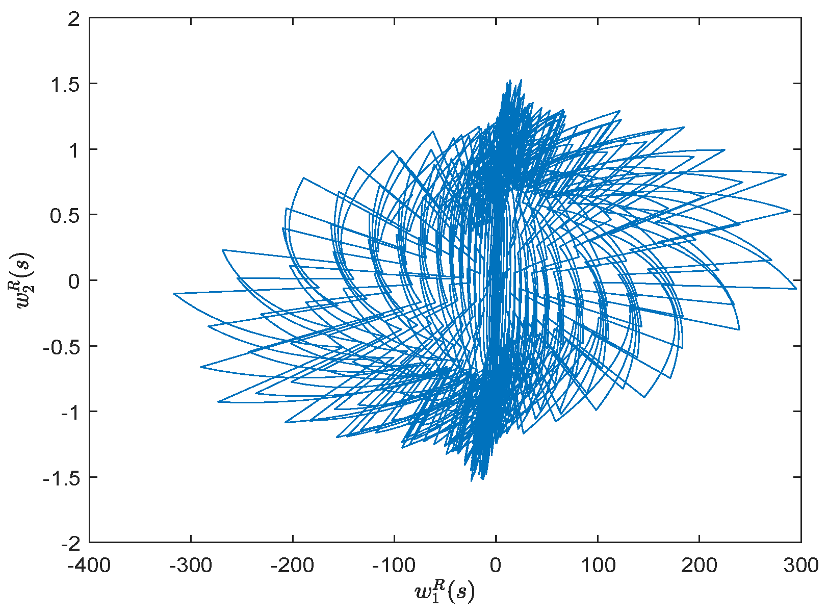
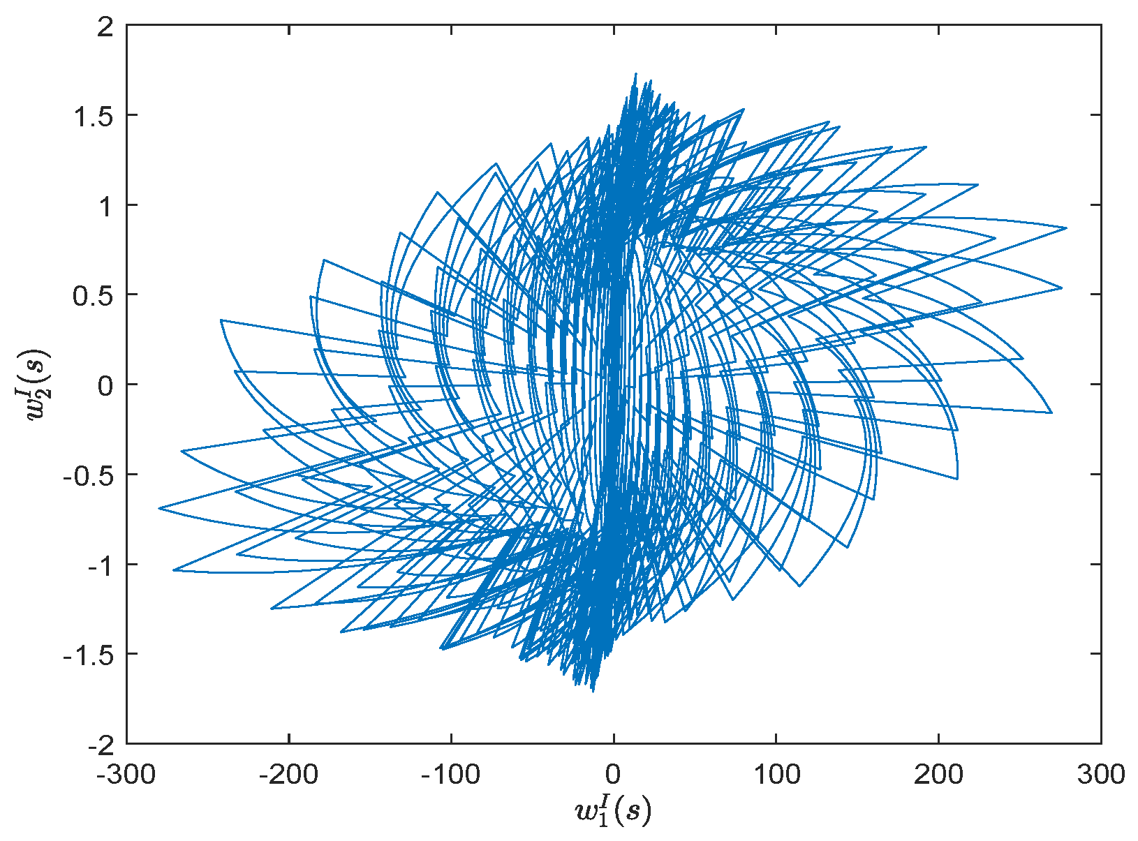
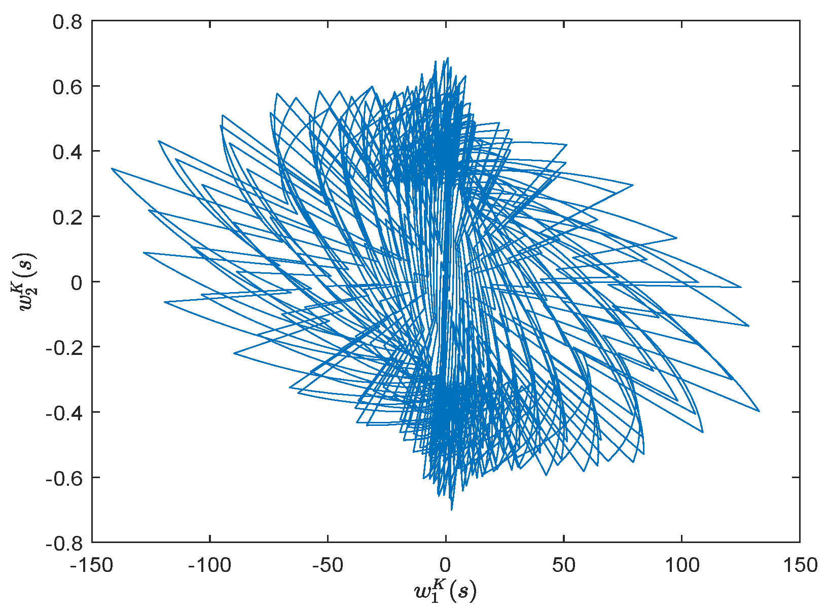
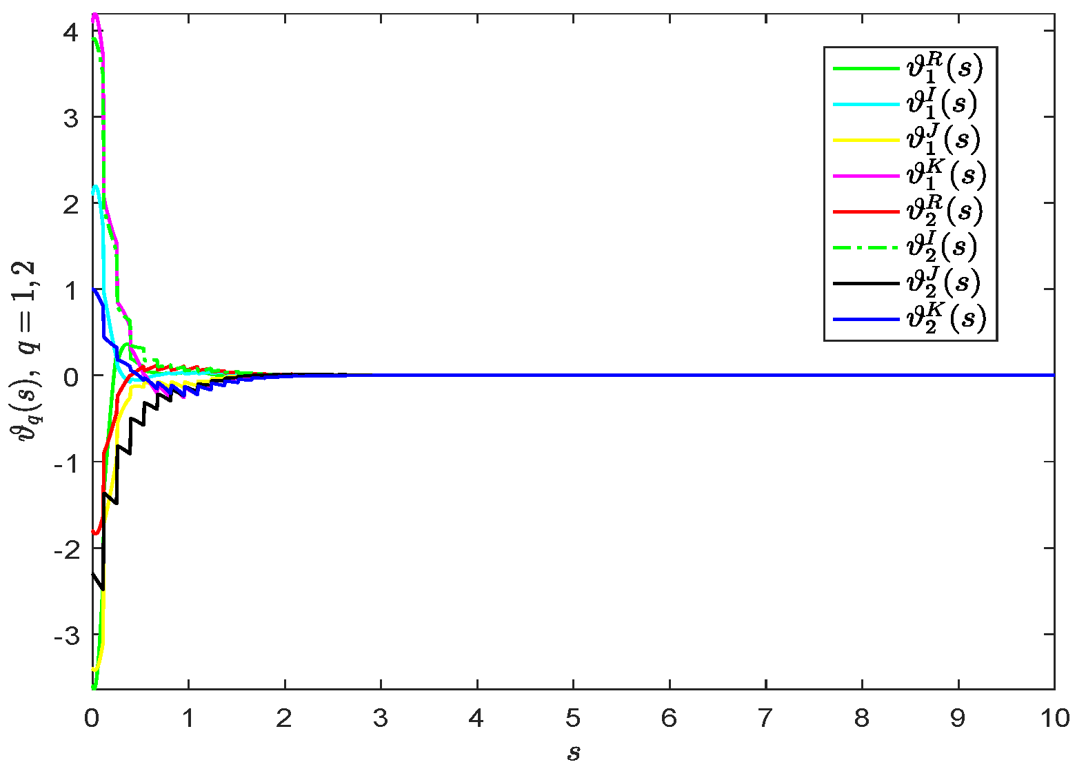
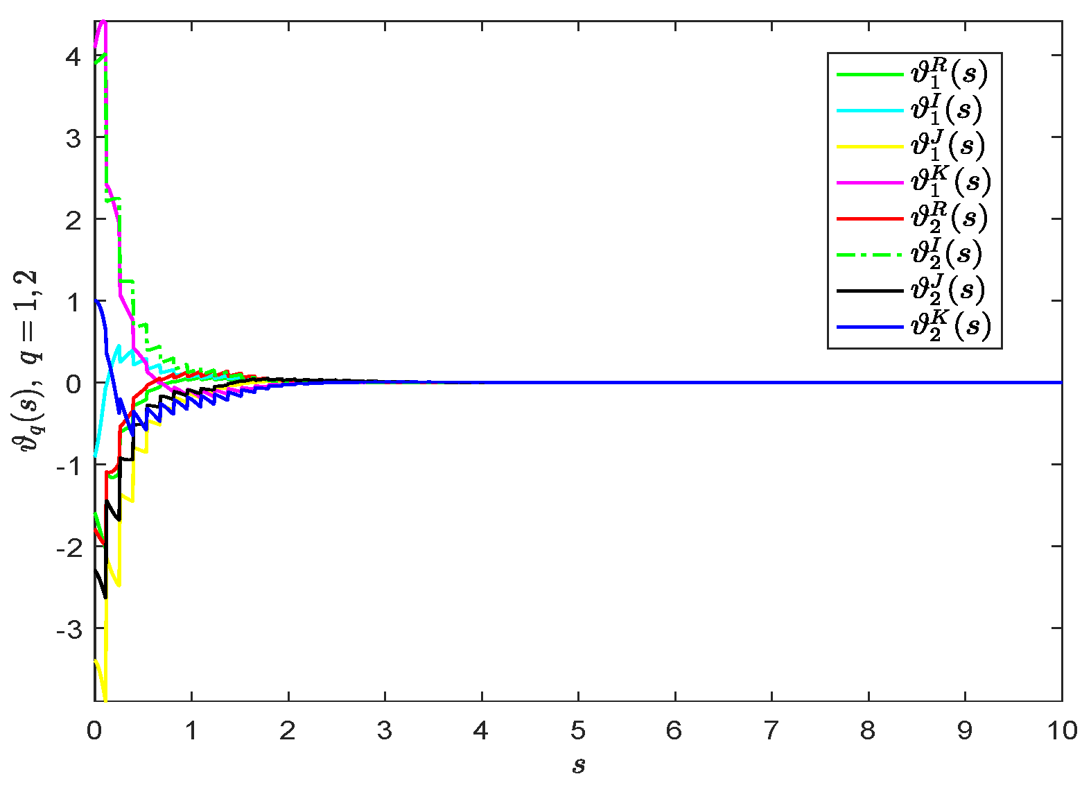
The dynamic evolution of the drive model (1) is given in Figure 1, Figure 2, Figure 3 and Figure 4, in which the initial values , for .

Figure 1.
Dynamic evolution of and .
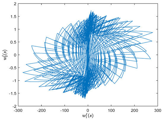
Figure 2.
Dynamic evolution of and .
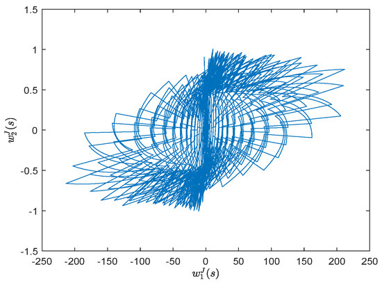
Figure 3.
Dynamic evolution of and .
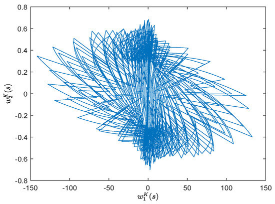
Figure 4.
Dynamic evolution of and .
Firstly, the synchronization between systems (1) and (3) is verified based on the control protocol (9). By simple calculation, , , . Set , , and ; then, by using the LMI toolbox in Matlab software, when , , and . So, by Theorem 1, systems (1) and (3) realize synchronization, which is revealed in Figure 5.
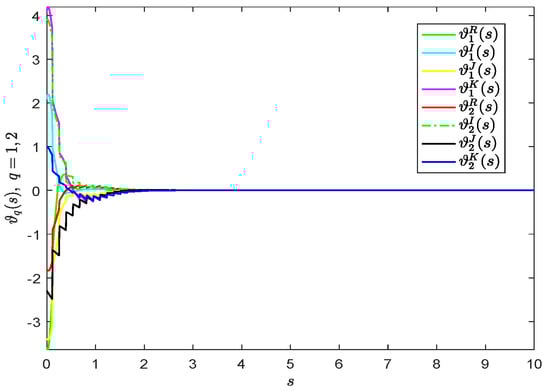
Figure 5.
The evolution of synchronization errors .
Next, adaptive synchronization will be verified. Choose , , and . By Theorem 3, systems (1) and (3) achieve adaptive synchronization via the adaptive control law (38), which is demonstrated by Figure 6 and Figure 7.

Figure 6.
The evolution of synchronization errors .
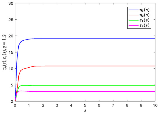
Figure 7.
The evolution of control gains and .
6. Conclusions
The synchronization problem of quaternion-valued delayed neural networks with impulse and inertia was studied in this paper. In all, a direct analysis method was developed to ensure synchronization, which is mainly reflected in two aspects. First of all, the control design is straightforward; that is, a kind of linear control scheme and its adaptive form were directly designed in the quaternion domain for the response quaternion-valued inertial systems, which are distinct from the control schemes for the reduced-order systems of inertial neural networks in [31,32] and the control strategies for subsystems obtained by separation used in [17,21,22,23]. Secondly, a convergence analysis is performed directly, that is, without separating the quaternion-valued systems into real-valued systems or transforming the inertial networks into first-order models, and some Lyapunov functionals are constructed directly based on the quaternion-valued error states and their derivatives to analyze the synchronization. In addition to developing a direct analysis technique, a generalization result of the Barbalat lemma is derived in Lemma 1. Here, the function is not necessarily differentiable everywhere; it provides a feasible method to investigate the stability of discontinuous models.
In addition to asymptotic synchronization, the fixed-time synchronization of INNs is also a hot issue at present [35,47,50]. However, there seems to be only a few reports on the fixed-time synchronization of QV-INNs with impulses based on the direct analysis approach. Moreover, as indicated in [10,27], the stochastic feature is universal in diverse fields including ecology, engineering and electrical systems, so it would be valuable to investigate the synchronization of stochastic QV-INNs with impulses. These interesting problems will be explored in a future study.
Author Contributions
Methodology, K.X. and C.H.; software, K.X.; validation, C.H.; formal analysis, J.Y.; writing—original draft, J.Y.; writing—review & editing, C.H.; supervision, C.H.; funding acquisition, C.H. All authors have read and agreed to the published version of the manuscript.
Funding
This research was funded by the National Natural Science Foundation of China (Grant Nos. 62263029 and 62373317), the Tianshan Talent Training Program (2022TSYCCX0013), the Key Project of Natural Science Foundation of Xinjiang (2021D01D10), Basic Research Foundation for Universities of Xinjiang (XJEDU2023P023) and the Intelligent Control and Optimization Research Platform at Xinjiang University.
Data Availability Statement
No new data were created or analyzed in this study. Data sharing is not applicable to this article.
Conflicts of Interest
The authors declare no conflicts of interest.
References
- Suissa, O.; Elmalech, A.; Zhitomirsky-Geffet, M. Text analysis using deep neural networks in digital humanities and information science. J. Assoc. Inf. Sci. Technol. 2022, 73, 268–287. [Google Scholar] [CrossRef]
- Shanmugam, L.; Mani, P.; Rajan, R.; Joo, Y. Adaptive synchronization of reaction-diffusion neural networks and its application to secure communication. IEEE Trans. Cybern. 2020, 50, 911–922. [Google Scholar] [CrossRef]
- Ullah, W.; Ullah, A.; Hussain, T.; Muhammad, K.; Heidari, A.; Ser, J.; Baik, S.; Albuquerque, V. Artificial intelligence of things-assisted two-stream neural network for anomaly detection in surveillance big video data. Future Gener. Comput. Syst. 2022, 129, 286–297. [Google Scholar] [CrossRef]
- Bill, J.; Champagne, L.; Cox, B.; Bihl, T. Meta-heuristic optimization methods for quaternion-valued neural networks. Mathematics 2021, 9, 938. [Google Scholar] [CrossRef]
- Zou, C.; Kou, K.; Wang, Y. Quaternion collaborative and sparse representation with application to color face recognition. IEEE Trans. Image Process. 2016, 25, 3287–3302. [Google Scholar] [CrossRef] [PubMed]
- Took, C.; Strba, G.; Aihara, K.; Mandic, D. Quaternion-valued short-term joint forecasting of three-dimensional wind and atmospheric parameters. Renew. Energy 2011, 36, 1754–1760. [Google Scholar] [CrossRef]
- Lin, Y.; Ling, B.; Hu, L.; Zheng, Y.; Xu, N.; Zhou, X.; Wang, X. Hyperspectral image enhancement by two dimensional quaternion valued singular spectrum analysis for object recognition. Remote Sens. 2021, 13, 405. [Google Scholar] [CrossRef]
- Wei, W.; Hu, C.; Yu, J.; Jiang, H. Fixed/preassinged-time synchronization of quaternion-valued neural networks involving delays and discontinuous activations: A direct approach. Acta Math. Sci. 2023, 43, 1439–1461. [Google Scholar] [CrossRef]
- Song, Q.; Yang, L.; Liu, Y.; Alsaadi, F. Stability of quaternion-valued neutral-type neural networks with leakage delay and proportional delays. Neurocomputing 2023, 521, 191–198. [Google Scholar] [CrossRef]
- Sathiyaraj, T.; Fečkan, M.; Wang, J. Synchronization of: Fractional Stochastic Chaotic Systems via Mittag–Leffler Function. Fractal Fract. 2022, 6, 192. [Google Scholar] [CrossRef]
- Zhang, T.; Jian, J. Quantized intermittent control tactics for exponential synchronization of quaternion-valued memristive delayed neural networks. ISA Trans. 2022, 126, 288–299. [Google Scholar] [CrossRef]
- Li, R.; Cao, J.; Xue, C.; Manivannan, R. Quasi-stability and quasi-synchronization control of quaternion-valued fractional-order discrete-time memristive neural networks. Appl. Math. Comput. 2021, 395, 125851. [Google Scholar] [CrossRef]
- Pu, H.; Li, F.; Wang, Q.; Li, P. Preassigned-time projective synchronization of delayed fully quaternion-valued discontinuous neural networks with parameter uncertainties. Neural Netw. 2023, 165, 740–754. [Google Scholar] [CrossRef] [PubMed]
- Peng, T.; Zhong, J.; Tu, Z.; Lu, J.; Lou, J. Finite-time synchronization of quaternion-valued neural networks with delays: A switching control method without decomposition. Neural Netw. 2022, 148, 37–47. [Google Scholar] [CrossRef] [PubMed]
- Wei, R.; Cao, J. Synchronization control of quaternion-valued memristive neural networks with and without event-triggered scheme. Cogn. Neurodyn. 2019, 13, 489–502. [Google Scholar] [CrossRef] [PubMed]
- Guo, J.; Shi, Y.; Luo, W.; Cheng, Y.; Wang, S. Adaptive global synchronization for a class of quaternion-valued cohen-grossberg neural networks with known or unknown parameters. Mathematics 2023, 11, 3553. [Google Scholar] [CrossRef]
- Zhang, Y.; Yang, L.; Kou, K.; Liu, Y. Fixed-time synchronization for quaternion-valued memristor-based neural networks with mixed delays. Neural Netw. 2023, 165, 274–289. [Google Scholar] [CrossRef] [PubMed]
- Wang, P.; Li, X.; Wang, N.; Li, Y.; Shi, K.; Lu, J. Almost periodic synchronization of quaternion-valued fuzzy cellular neural networks with leakage delays. Fuzzy Setsand Syst. 2022, 426, 46–65. [Google Scholar] [CrossRef]
- Mao, X.; Wang, X.; Qin, H. Stability analysis of quaternion-valued BAM neural networks fractional-order model with impulses and proportional delays. Neurocomputing 2022, 509, 206–220. [Google Scholar] [CrossRef]
- Shu, J.; Xiong, L.; Wu, T.; Liu, Z. Stability analysis of quaternion-valued neutral-type neural networks with time-varying delay. Mathematics 2019, 7, 101. [Google Scholar] [CrossRef]
- Wei, W.; Yu, J.; Wang, L.; Hu, C.; Jiang, H. Fixed/Preassigned-time synchronization of quaternion-valued neural networks via pure power-law control. Neural Netw. 2022, 146, 341–349. [Google Scholar] [CrossRef]
- Deng, H.; Bao, H. Fixed-time synchronization of quaternion-valued neural networks. Phys. A Stat. Mech. Its Appl. 2019, 527, 121351. [Google Scholar] [CrossRef]
- Qi, X.; Bao, H.; Cao, J. Synchronization criteria for quaternion-valued coupled neural networks with impulses. Neural Netw. 2020, 128, 150–157. [Google Scholar] [CrossRef] [PubMed]
- Li, R.; Gao, X.; Cao, J. Quasi-state estimation and quasi-synchronization control of quaternion-valued fractional-order fuzzy memristive neural networks: Vector ordering approach. Appl. Math. Comput. 2019, 362, 124572. [Google Scholar] [CrossRef]
- Peng, T.; Lu, J.; Xiong, J.; Tu, Z.; Liu, Y.; Lou, J. Fixed-time synchronization of quaternion-valued neural networks with impulsive effects: A non-decomposition method. Commun. Nonlinear Sci. Numer. Simul. 2024, 132, 107865. [Google Scholar] [CrossRef]
- Babcock, K.; Westervelt, R. Stability and dynamics of simple electronic neural networks with added inertia. Phys. D Nonlinear Phenom. 1986, 23, 464–469. [Google Scholar] [CrossRef]
- Dhayal, R.; Malik, M.; Abbas, S.; Debbouche, A. Optimal controls for second-order stochastic differential equations driven by mixed-fractional Brownian motion with impulses. Math. Methods Appl. Sci. 2020, 43, 4107–4124. [Google Scholar] [CrossRef]
- Chang, S.; Wang, Y.; Zhang, X.; Wang, X. A new method to study global exponential stability of inertial neural networks with multiple time-varying transmission delays. Math. Comput. Simul. 2023, 211, 329–340. [Google Scholar] [CrossRef]
- Duan, L.; Li, J. Global exponential bipartite synchronization for neutral memristive inertial coupling mixed time-varying delays neural networks with antagonistic interactions. Commun. Nonlinear Sci. Numer. Simul. 2023, 119, 107071. [Google Scholar] [CrossRef]
- Yao, Y.; Zhang, G.; Li, Y. Fixed/Preassigned-time stabilization for complex-valued inertial neural networks with distributed delays: A non-separation approach. Mathematics 2023, 11, 2275. [Google Scholar] [CrossRef]
- Li, Q.; Zhou, L. Global asymptotic synchronization of inertial memristive Cohen–Grossberg neural networks with proportional delays. Commun. Nonlinear Sci. Numer. Simul. 2023, 123, 107295. [Google Scholar] [CrossRef]
- Yao, W.; Wang, C.; Sun, Y.; Gong, S.; Lin, H. Event-triggered control for robust exponential synchronization of inertial memristive neural networks under parameter disturbance. Neural Netw. 2023, 164, 67–80. [Google Scholar] [CrossRef]
- Li, X.; Li, X.; Hu, C. Some new results on stability and synchronization for delayed inertial neural networks based on non-reduced order method. Neural Netw. 2017, 96, 91–100. [Google Scholar] [CrossRef]
- Chen, S.; Jiang, H.; Hu, C.; Li, L. Cluster synchronization for directed coupled inertial reaction-diffusion neural networks with nonidentical nodes via non-reduced order method. J. Frankl. Inst. 2023, 360, 3208–3240. [Google Scholar] [CrossRef]
- Han, J.; Chen, G.; Wang, L.; Zhang, G.; Hu, J. Direct approach on fixed-time stabilization and projective synchronization of inertial neural networks with mixed delays. Neurocomputing 2023, 535, 97–106. [Google Scholar] [CrossRef]
- Wang, J.; Tian, Y.; Hua, L.; Shi, K.; Zhong, S.; Wen, S. New results on finite-time synchronization control of chaotic memristor-based inertial neural networks with time-varying delays. Mathematics 2023, 11, 684. [Google Scholar] [CrossRef]
- Shanmugasundaram, S.; Kashkynbayev, A.; Udhayakumar, K.; Rakkiyappan, R. Centralized and decentralized controller design for synchronization of coupled delayed inertial neural networks via reduced and non-reduced orders. Neurocomputing 2022, 469, 91–104. [Google Scholar] [CrossRef]
- Shi, J.; Zeng, Z. Global exponential stabilization and lag synchronization control of inertial neural networks with time delays. Neural Netw. 2020, 126, 11–20. [Google Scholar] [CrossRef] [PubMed]
- Wei, R.; Cao, J.; Abdel-Aty, M. Fixed-time synchronization of second-order MNNs in quaternion field. IEEE Trans. Syst. Man Cybern. Syst. 2021, 51, 3587–3598. [Google Scholar] [CrossRef]
- Zhang, Z.; Wang, S.; Wang, X.; Wang, Z.; Lin, C. Event-triggered synchronization for delayed quaternion-valued inertial fuzzy neural networks via non-reduced order approach. IEEE Trans. Fuzzy Syst. 2023, 31, 3000–3014. [Google Scholar] [CrossRef]
- Xiong, K.; Hu, C.; Yu, J. Direct approach-based synchronization of fully quaternion-valued neural networks with inertial term and time-varying delay. Chaos Solitons Fractals 2023, 172, 113556. [Google Scholar] [CrossRef]
- Yang, Y.; Cao, J. Stability and periodicity in delayed cellular neural networks with impulsive effects. Nonlinear Anal. Real World Appl. 2007, 8, 362–374. [Google Scholar] [CrossRef]
- Vivek, S.; Vijayakumar, V. An analysis on the approximate controllability of neutral functional hemivariational inequalities with impulses. Optimization 2023. [Google Scholar] [CrossRef]
- Zhang, Y.; Zhou, L. Stabilization and lag synchronization of proportional delayed impulsive complex-valued inertial neural networks. Neurocomputing 2022, 507, 428–440. [Google Scholar] [CrossRef]
- Lin, D.; Chen, X.; Yu, G.; Li, Z.; Xia, Y. Global exponential synchronization via nonlinear feedback control for delayed inertial memristor-based quaternion-valued neural networks with impulses. Appl. Math. Comput. 2021, 401, 126093. [Google Scholar] [CrossRef]
- Wei, X.; Zhang, Z.; Lin, C.; Chen, J. Synchronization and anti-synchronization for complex-valued inertial neural networks with time-varying delays. Appl. Math. Comput. 2021, 403, 126194. [Google Scholar] [CrossRef]
- Long, C.; Zhang, G.; Hu, J. Fixed-time synchronization for delayed inertial complex-valued neural networks. Appl. Math. Comput. 2021, 405, 126272. [Google Scholar] [CrossRef]
- Popov, V. Hyperstability of Control Systems; Springer: New York, NY, USA, 1973. [Google Scholar]
- Jiang, H. Hybrid adaptive and impulsive synchronisation of uncertain complex dynamical networks by the generalised Barbalat’s lemma. IET Control Theory Appl. 2009, 3, 1330–1340. [Google Scholar] [CrossRef]
- Wei, F.; Chen, G.; Zeng, Z.; Gunasekaran, N. Finite/fixed-time synchronization of inertial memristive neuralnetworks by interval matrix method for secure communication. Neural Netw. 2023, 167, 168–182. [Google Scholar] [CrossRef]


Disclaimer/Publisher’s Note: The statements, opinions and data contained in all publications are solely those of the individual author(s) and contributor(s) and not of MDPI and/or the editor(s). MDPI and/or the editor(s) disclaim responsibility for any injury to people or property resulting from any ideas, methods, instructions or products referred to in the content. |
© 2024 by the authors. Licensee MDPI, Basel, Switzerland. This article is an open access article distributed under the terms and conditions of the Creative Commons Attribution (CC BY) license (https://creativecommons.org/licenses/by/4.0/).