Sparse Estimation for Hamiltonian Mechanics

Abstract

Estimating governing equations from observed time-series data is crucial for understanding dynamical systems. From the perspective of system comprehension, the demand for accurate estimation and interpretable results has been particularly emphasized. Herein, we propose a novel data-driven method for estimating the governing equations of dynamical systems based on machine learning with high accuracy and interpretability. The proposed method enhances the estimation accuracy for dynamical systems using sparse modeling by incorporating physical constraints derived from Hamiltonian mechanics. Unlike conventional approaches used for estimating governing equations for dynamical systems, we employ a sparse representation of Hamiltonian, allowing for the estimation. Using noisy observational data, the proposed method demonstrates a capability to achieve accurate parameter estimation and extraction of essential nonlinear terms. In addition, it is shown that estimations based on energy conservation principles exhibit superior accuracy in long-term predictions. These results collectively indicate that the proposed method accurately estimates dynamical systems while maintaining interpretability.

1. Introduction

Recent advances in measurement and information technologies have improved the quantity and quality of available data. Owing to these improvements, data-driven approaches have attracted attention as a method to extract the system structure and features from data [1,2,3]. Notably, the extraction of dynamical systems from time-series data is challenging in various fields, encompassing natural sciences, such as earth science [4,5] and neuroscience [6,7], and engineering domains, such as fluid engineering [8,9,10]. Moreover, methods for state estimation have been proposed for various systems ranging from physical systems with unknown governing equations to networked autonomous vehicles with event-triggered control, robustness against disturbances, and time-varying delays [11,12].

Typical data-driven approaches include methods using Bayesian estimation [13,14,15,16,17,18] and deep learning [19,20,21,22,23,24]. Bayesian estimation is used to estimate the parameters of a model but requires a certain modeling and cannot deal with completely unknown mechanisms. Meanwhile, deep learning can extract dynamical systems from only observed data; however, there are concerns about reduced interpretability due to black-box estimation.

Sparse-estimation-based methods have been considered to address these concerns [25,26,27,28,29,30,31,32]. In these methods, a set of candidate basis functions is prepared in advance, and basis selection and coefficient estimation are performed through optimization. This approach does not require complete modeling of phenomena and is highly interpretable because the constitutive equations of the dynamical system are available. However, it is difficult to extract precise dynamical models even with conventional sparse methods when considering long-term forecasts with noisy data.

Herein, we propose a new sparse-estimation method that introduces constraints based on physical laws. The proposed method achieves sparse estimation based on Hamiltonian dynamical systems. As a result, it can make predictions based on the energy conservation law and extract dynamical systems that achieve stable simulation results in the long term.

The key difference between the proposed method and conventional methods [25] is in their main target of estimation. Conventional methods perform estimation for each governing equation individually, whereas the proposed method performs estimation regarding Hamiltonian. As a consequence, conventional methods require individual estimations for each state variable, making the estimation difficult as the number of variables increases. In contrast, the proposed method simplifies the estimation by considering the estimation of only a single parameter, regardless of the number of state variables. Furthermore, the proposed method focuses on Hamiltonian to obtain energetically stable and accurate state estimation results. By incorporating Hamiltonian into the estimation, the proposed method considers essential information on physical formula, which distinguishes the proposed method from the conventional methods.

The proposed method assumes the sparse representation of Hamiltonian, while the observational data may satisfy the dynamical equations derived from the Hamiltonian rather than the sparse representation of the Hamiltonian itself. Therefore, it had been unclear how the machine-learning formulation of the dynamical system can be realized with a physically plausible formulation such as Hamiltonian. To overcome such difficulty, the proposed method mathematically combines the machine-learning formulation of the dynamical system with the physically plausible formulation described by Hamiltonian.

The remainder of this article is organized as follows. In Section 2, we propose a sparse model based on Hamiltonian dynamical systems. For illustration, we also describe the techniques underlying the proposed method: Hamiltonian dynamics and sparse estimation of conventional dynamical systems. Next, the proposed method is described in detail. In Section 3, we present the results of a comparison of the proposed method with two conventional methods that are unconstrained by physical laws to validate our method. First, we compare the estimation results for two systems: the Duffing oscillator and Rayleigh–Bénard convection. Second, we verify the robustness of our method against noise. Concluding remarks are given in Section 4, where the effectiveness of the proposed method is discussed and perspectives for future work are given.

2. Methods

In this section, we propose a data-driven method for estimating the governing equations of dynamical equations from time-series data. First, we describe Hamiltonian mechanics. Next, we describe the conventional approach for estimating dynamical systems with sparse estimation. Thereafter, we propose the sparse-estimation method by imposing the physical information possessed by Hamiltonian dynamics as a constraint to improve accuracy. The notation of symbols used in this paper is summarized in Appendix A.

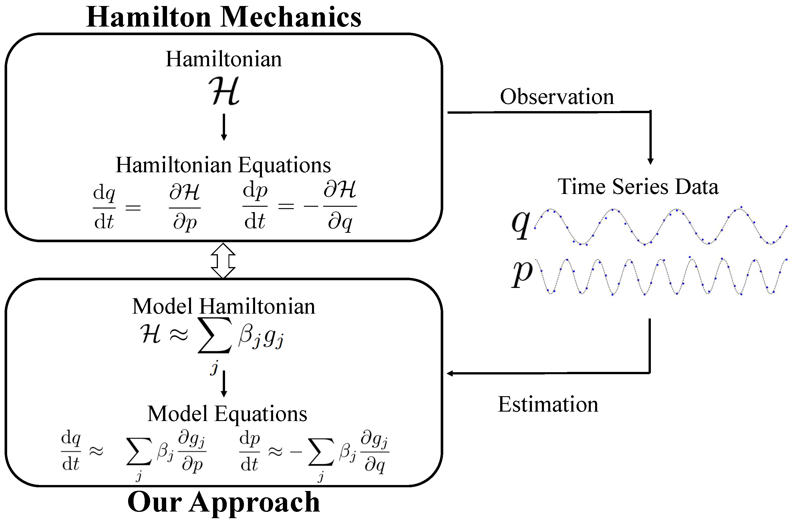
2.1. Hamiltonian Mechanics

Hamiltonian mechanics offers a framework for describing the time evolution of states of physical systems that admit the law of conservation of energy. In Hamiltonian mechanics, governing dynamics is mathematically formulated by two independent variables: generalized coordinates $\mathit{q}=[q_1,\dots ,q_n]$ and generalized momenta $\mathit{p}=[p_1,\dots ,p_n]$, where n is the system’s degree of freedom. Using these variables, the system’s dynamical behavior is described by the following equations:

$$\frac{\mathrm{d}{q}_i}{\mathrm{d}t}=\frac{\partial \mathcal{H}(\mathit{p},\mathit{q},t)}{\partial p_i},\frac{\mathrm{d}{p}_i}{\mathrm{d}t}=-\frac{\partial \mathcal{H}(\mathit{p},\mathit{q},t)}{\partial q_i},\mathrm{for}i=1,\dots ,n,$$

(1)

where $\mathcal{H}=\mathcal{H}(\mathit{p},\mathit{q},t)$ is called Hamiltonian, which is a function of $\mathit{q}$ and $\mathit{p}$ that represents the energy of the entire system. Using Hamiltonian, the system can be expressed symmetrically. Further, if the Hamiltonian does not explicitly depend on time ($\mathcal{H}=\mathcal{H}(\mathit{p},\mathit{q})$), the relation $\mathrm{d}\mathcal{H}/\mathrm{d}t=0$ holds, i.e., the conservation of energy is guaranteed. In addition, the Noether theorem asserts that the symmetry of the system leads to a conservation law. The Hamilton equations include the Newton equation and can describe broader physical phenomena in a manner consistent with the original laws of nature.

2.2. Sparse Estimation for Dynamical Systems

Sparse estimation of dynamical systems is a method that can be applied even when the model is unknown. This is because the method allows the selection of basis functions in the optimization by sparsely estimating the coefficients under the condition that the candidate basis functions have been prepared in advance. Assuming that m basis functions $\{g_1(·),\dots ,g_m(·)\}$ are prepared, the following basis decomposition is considered for the governing equation of the state variable y:

$$\frac{\mathrm{d}y}{\mathrm{d}t}\approx \sum _{j=1}^m{\mu }_j{g}_j(y,t).$$

(2)

The following objective functions are considered to estimate the sparse coefficient $\mathit{\mu }=[{\mu }_1,\dots ,{\mu }_m]$ corresponding to the basis functions:

$$\mathcal{L}\left(\mathit{\mu }\right)={∥\frac{\mathrm{d}y}{\mathrm{d}t}-\sum _{j=1}^m{\mu }_j{g}_j(y,t)∥}_2^2+\lambda {∥\mathit{\mu }∥}_1,$$

(3)

where ${\parallel ·\parallel }_2$ and ${\parallel ·\parallel }_1$ are $L_2$ and $L_1$ norms, respectively. This optimization leads to the extraction of an essential basis from a set of a priori basis functions. Therefore, both prediction and interpretation of the dynamical system by extracting the governing equations can be realized.

2.3. Proposed Method

In this study, we develop a data-driven method for estimating dynamical equations from time-series data (Figure 1). The proposed method outputs the Hamiltonian model and system response from noisy observational data by imposing constraints consisting of sparse constraints and property of Hamiltonian mechanics (Figure 2).

In particular, constraints related to the properties of the Hamiltonian dynamical system serve as physical constraints. By imposing the physical constraint, dynamical equations (Equation (1)) can be expressed for all dimension i as follows:

$$\frac{\mathrm{d}{q}_i}{\mathrm{d}t}\approx \sum _{j=1}^m{\beta }_j\frac{\partial g_j(\mathit{q},\mathit{p},t)}{\partial p_i},\frac{\mathrm{d}{p}_i}{\mathrm{d}t}\approx -\sum _{j=1}^m{\beta }_j\frac{\partial g_j(\mathit{q},\mathit{p},t)}{\partial q_i},$$

(4)

where $g_1(\mathit{q},\mathit{p},t),\dots ,g_m(\mathit{q},\mathit{p},t)$ are nonlinear functions that can be candidates for the m basis functions prepared in advance and $\mathit{\beta }=[{\beta }_1,\dots ,{\beta }_m]$ is the weight coefficient.

Notably, a single common coefficient, ${\beta }_j$, is applied to two equations for $\mathrm{d}{q}_i/\mathrm{d}t$ and $\mathrm{d}{p}_i/\mathrm{d}t$ with subscript j, and this common property holds for all subscript j and even for all degrees of freedom. This commonality can be achieved by decomposing Hamiltonian $\mathcal{H}$ into m terms as follows:

$$\mathcal{H}\approx \sum _{j=1}^m{\beta }_j{g}_j(\mathit{q},\mathit{p},t).$$

(5)

When using the Hamiltonian to represent Equation (4), because the weight coefficients are independent of $\mathit{q}$, $\mathit{p}$, and time t, the partial differentiation can be moved to the basis function components. Moreover, the partial derivatives of the basis functions can be easily calculated either analytically or numerically, assuming that the functions are known.

To extract only essential nonlinear terms, we propose a sparse modeling approach for Hamiltonian dynamics. We assume that the state values $\mathit{q}$, $\mathit{p}$ and their time derivatives $\mathrm{d}\mathit{q}/\mathrm{d}t$, $\mathrm{d}\mathit{p}/\mathrm{d}t$ are given as data. State values are used to create nonlinear basis functions constituting the Hamiltonian approximation, whereas time derivatives serve as objective variables. The objective function is as follows:

$$\mathcal{L}\left(\mathit{\beta }\right)={∥\left[\begin{array}{c}{\dot{\mathit{q}}}_{\mathrm{obs}}\\ {\dot{\mathit{p}}}_{\mathrm{obs}}\end{array}\right]-\sum _{j=1}^m{\beta }_j\left[\begin{array}{c}\frac{\partial g_j({\mathit{q}}_{\mathrm{obs}},{\mathit{p}}_{\mathrm{obs}},t)}{\partial \mathit{p}}\\ -\frac{\partial g_j({\mathit{q}}_{\mathrm{obs}},{\mathit{p}}_{\mathrm{obs}},t)}{\partial \mathit{q}}\end{array}\right]∥}_2^2+\lambda {\parallel \mathit{\beta }\parallel }_1,$$

(6)

where ${\mathit{q}}_{\mathrm{obs}}$ and ${\mathit{p}}_{\mathrm{obs}}$ denote the observed values of $\mathit{q}$ and $\mathit{p}$, respectively, and ${\dot{\mathit{q}}}_{\mathrm{obs}}{\dot{\mathit{p}}}_{\mathrm{obs}}$ denote the observed values of $\mathrm{d}\mathit{q}/\mathrm{d}t$, $\mathrm{d}\mathit{p}/\mathrm{d}t$, respectively. $L_1$-norm regularization is introduced for the weight coefficients, $\mathit{\beta }$, for sparse estimation. The regularization parameter, $\lambda$, determines the sparsity strength. Using the objective function (Equation (6)), the shared coefficients, ${\mathit{\beta }}^{★}$, are estimated as follows:

$${\mathit{\beta }}^{★}=\underset{\mathit{\beta }}{argmin}\mathcal{L}\left(\mathit{\beta }\right).$$

(7)

By assuming sparse representation in Hamiltonian $\mathcal{H}(\mathit{q},\mathit{p})$, we realize simultaneous estimation of dynamical equations for $\mathit{q}$ and $\mathit{p}$. Further, this sparsity reduces the dimension, leading to a lightweight simulation. This allows only terms related to the Hamiltonian to be extracted from a large number of basis functions, contributing to the identification of dynamics and the interpretability of the model.

Finally, we highlight the distinctions between the conventional approach and our approach. The conventional approach (Equation (2)) requires that the Hamilton equation (Equation (1)) be formulated as follows:

$$\frac{\mathrm{d}{q}_i}{\mathrm{d}t}\approx \sum _{j=1}^m{\mu }_{i,j}{g}_j(\mathit{q},\mathit{p},t),\frac{\mathrm{d}{p}_i}{\mathrm{d}t}\approx \sum _{j=1}^m{\nu }_{i,j}{g}_j(\mathit{q},\mathit{p},t),$$

(8)

where ${\mu }_{i,j}$ and ${\nu }_{i,j}$ are independent multiple coefficients corresponding to $\mathrm{d}{q}_i/\mathrm{d}t$ and $\mathrm{d}{p}_i/\mathrm{d}t$, respectively. This means that the estimation is based only on data and is performed independently for each state variable and degree of freedom. Meanwhile, regarding Equation (4), it is possible to relate the equations according to physical laws. From this, it can be argued that our proposed approach considering Hamiltonian mechanics (Equations (4)–(6)) can introduce regularization based on physical laws. The code for the proposed method is summarized in Appendix B.

3. Results

To evaluate the performance of the proposed method, we employed it to estimate the dynamical systems from simulated data for two Hamiltonian dynamical systems: the Duffing oscillator and Rayleigh–Bénard convection.

To demonstrate the effectiveness of the proposed method, we employed the least-squares method without regularization (LSM) and the least-squares method with $L_1$-norm regularization (LASSO) for comparison. LSM and LASSO do not consider Hamiltonian mechanics and use the time derivatives of the state variables as objective variables. The evaluation criteria comprise assessing the accuracy of the estimated weight coefficients and comparing the accuracy of the long-term forecasts. For the long-term forecasts, nonlinear behavior was reconstructed from the estimated coefficients and basis functions to obtain the predicted values. The predicted values were obtained through numerical analysis, and their discrepancies with the true values were examined. In this case, the Dormand–Prince method implemented in SciPy [33], a Python library, was used for numerical analysis. For numerical analysis, the tolerance for absolute and relative errors was set to be ${10}^{-10}$. During learning, it is assumed that a set of candidate functions containing the correct basis functions is prepared based on prior knowledge. In the proposed method, numerical partial differentiation by central differencing was employed in the operations regarding the basis functions of the proposed method. To achieve optimal sparsity, the regularization parameters were automatically selected to achieve the best generalization performance of the proposed method and LASSO.

3.1. Duffing Oscillator

A Duffing oscillator is a nonlinear oscillator whose oscillations are characterized by nonlinear terms. We consider the following Hamiltonian:

$$\mathcal{H}(p,q)=\frac{1}{2}{p}^2+\frac{1}{2}a{q}^2+\frac{1}{4}b{q}^4,$$

(9)

where we consider that the system does not have a dissipative term and hence conserves energy. In Equation (9), we assume that the true parameter values are $a=1$ and $b=1.5$; it is known that when both a and b are positive we have a bounded solution [34]. For the observed values, data were prepared at a time interval of 0.001 from $t=0$ to 20. The first $25\%$ of the data points were used for training, which corresponds to approximately 1.75 cycles (1000 data points), whereas the remaining $75\%$ were used for testing. Gaussian noise with a mean of 0 and variance of 0.01 ($\mathcal{N}(0,0.01)$) was added to the state values, and $\mathcal{N}(0,1)$ was added to the time derivatives of the state values. The following 10 candidate basis functions were prepared:

$$\left\{q^u,p^u\mid u\in \mathbb{N},1\le u\le 5\right\},$$

where these candidate basis functions are the first to the fifth power of each state variable q and p.

Figure 3 shows the estimated coefficients of the basis functions for each method. The true coefficients to be estimated are represented by black dots and the estimated results are represented by blue circles. For LSM, discrepancies between the estimated and true values occur when the true values are both zero and nonzero. Similar discrepancies occurred for LASSO, especially when the true values were nonzero. Moreover, in LSM and LASSO, the coefficients that should have the same value between q and p did not match. Meanwhile, the proposed method estimated the coefficients more accurately, indicating the proposed method’s effectiveness.

The results of the long-term predictions are shown in Figure 4. The behavior of true state values is represented by black dotted lines, predictions for training data are represented by light blue dots, and predictions for test data are represented by red crosses. LSM and LASSO initially yielded results close to the true trajectory; however, the closeness decayed over time, leading to large deviations. This is due to the accumulation of errors in the numerical calculations generated by incorrectly estimated dynamical equations, indicating that discrepancies in time derivatives and estimated coefficients lead to large deviations. Meanwhile, the proposed method estimated values closer to the true values; in particular, it showed a stable trajectory with unchanging amplitudes, indicating that the proposed method can achieve estimations that adequately reflect the energy conservation law of Hamiltonian.

Finally, for quantitative evaluation, the root mean squared error (RMSE) of the long-term prediction is summarized in

Table 1. Comparison of RMSE. The lowest RMSE values for each demonstration are shown in bold.

	Duffing Oscillator	Rayleigh–Bénard Convection
Ours	0.19	0.26
LSM	1.82	1.51
LASSO	1.39	2.09

. The proposed method has only a slight error due to a slight phase delay, whereas LSM and LASSO have large errors relative to the true dynamic range due to amplitude decay.

3.2. Rayleigh–Bénard Convection

Rayleigh–Bénard convection is an important phenomenon in fluid dynamics, particularly contributing to our understanding of natural convection [35]. This phenomenon can be observed in very simple situations and has been the subject of many theoretical and experimental investigations. In this study, the following Hamiltonian is considered:

$$\mathcal{H}(p,q)=\frac{A}{k}sin\left(kp\right)sin\left(\pi q\right),$$

(10)

where we consider an energy-stable system. We assume that the true parameter values are set to be $A=7.1$ and $k=1.2$ in Equation (10). For the observed values, the data were prepared at 0.001 time intervals from $t=0$ to $19.2$, which is for 38.4 cycles. The first half of the data points were used for training and the other half were used for testing. As noise, $\mathcal{N}(0,0.01)$ was added to the state values and $\mathcal{N}(0,0.5)$ was added to the time derivatives of the state values. The following 54 candidate basis functions were prepared:

$$\begin{array}{cc}\hfill & \left\{sin\left(\omega t\right)sin\left(ukp\right)sin\left(\pi q\right),cos\left(\omega t\right)sin\left(ukp\right)sin\left(\pi q\right),sin\left(\omega t\right)cos\left(ukp\right)sin\left(\pi q\right),\right.\hfill \\ \hfill & cos\left(\omega t\right)cos\left(ukp\right)sin\left(\pi q\right),sin\left(\omega t\right)sin\left(ukp\right)cos\left(\pi q\right),cos\left(\omega t\right)sin\left(ukp\right)cos\left(\pi q\right),\hfill \\ \hfill & sin\left(\omega t\right)cos\left(ukp\right)cos\left(\pi q\right),cos\left(\omega t\right)cos\left(ukp\right)cos\left(\pi q\right),sin\left(\omega t\right),sin\left(\omega t\right)p,sin\left(\omega t\right)q,\hfill \\ \hfill & cos\left(\omega t\right),cos\left(\omega t\right)p,cos\left(\omega t\right)q,sin\left(ukp\right)sin\left(\pi q\right),cos\left(ukp\right)sin\left(\pi q\right),sin\left(ukp\right)cos\left(\pi q\right),\hfill \\ \hfill & \left.cos\left(ukp\right)cos\left(\pi q\right)\mid u\in \mathbb{N},1\le u\le 4,\omega =2\pi /T\right\}.\hfill \end{array}$$

(11)

The estimated basis function coefficients for each method are shown in Figure 5. The true coefficients to be estimated are represented by black dots and the estimated results by blue circles. Because of the large number of candidate basis functions, LSM estimates basis function coefficients with large values, resulting in equations that differ significantly from the original governing equations and LASSO estimates coefficients with small absolute values, which also differ from the original governing equations. Meanwhile, the proposed method selects only the appropriate basis, and its coefficients are estimated correctly. Compared with LASSO, the proposed method can estimate the coefficients between the state variables independently and is thus able to estimate them correctly, even when there are many candidate basis functions.

Figure 6 shows the results of the long-term prediction. The behavior of true state values is represented by black dotted lines, predictions for training data by light blue dots, and predictions for test data by red crosses. As in the case of the Duffing oscillator, LSM and LASSO initially exhibit amplitudes close to the true trajectory; however, they deviate from the true system and converge to a certain point over time. Meanwhile, the proposed method maintains the amplitudes and exhibits a stable trajectory that is closer to the true behavior, indicating that it correctly estimates the coefficients and is based on the law of conservation of energy.

For quantitative evaluation, Table 1 summarizes the RMSE of the long-term forecasts. Both LSM and LASSO have large errors relative to the true dynamic range, although there is a difference in the values due to the convergence points. Meanwhile, the proposed method has only a small error due to the phase delay, as in the case of the Duffing oscillator.

3.3. Robustness

Here, we verify the robustness of the proposed method against noise. For verification, the Duffing oscillator discussed in Section 3.1 was subjected to Gaussian noise with variances of magnitudes 0%, 1%, 2%, 3%, 4%, 5%, 7%, and 10% of the amplitude for each of the time derivatives of the state value. The methods used for comparison were LSM and LASSO.

The comparison results of the trends of noise magnitude and the RMSE for each method are shown in Figure 7. The results for the proposed method are shown as red circles and solid lines, those for LSM as green crosses and dotted lines, and those for LASSO as blue triangles and dashed lines. LSM yielded accurate results in the absence of noise but yielded large errors with small amounts of noise and significantly larger errors as the noise level increased. LASSO showed a smaller error than LSM but similarly yielded larger errors with increasing noise. Meanwhile, the proposed method maintained an error of <0.1, even as the noise level increased; the error tended to increase only slightly. Even for 1% noise, the RMSE values of the conventional methods were large, whereas the proposed method showed a small RMSE value, even for 10% noise. This indicates that the proposed method is highly robust against noise.

4. Conclusions

Herein, we propose a sparse modeling method based on Hamiltonian mechanics and estimate the sparse representation of Hamiltonian to achieve accurate simulations of dynamical systems in the long term. The proposed method can extract governing equations from observed data even when the system model is unknown. The proposed method enables extraction that is stable on a long-term periodic basis through estimation that considers the law of conservation of energy of the system, which is represented by the time invariance of the Hamiltonian, a property of Hamiltonian mechanics.

Using nonlinear dynamical models of the Duffing oscillator and Rayleigh–Bénard convection, we show that the proposed method is more effective than existing methods that do not consider Hamiltonian dynamical systems. The proposed method has better system estimation accuracy than existing methods for long-term system behavior reproduction. In particular, the proposed method correctly estimates the Hamiltonian coefficients even when the number of basis functions is large. Further, when comparing noise magnitude and long-term prediction accuracy for the Duffing oscillator, the existing methods, which do not consider the dynamical system, show a tendency of decreasing accuracy with increasing noise, whereas the proposed method maintains high accuracy. This indicates that the proposed method is highly robust against noise.

In this paper, we have shown the effectiveness of the proposed method using noisy observable data where the noise obeys Gaussian distribution. It is known that the sparse estimation used in the proposed method can achieve accurate estimation or noisy observable data regardless of whether the noise obeys Gaussian distribution or non-Gaussian distribution [36]. Therefore, we believe that the proposed method is also effective for data with noise following non-Gaussian distributions. Based on the above results, the proposed method is evaluated to have achieved better estimation accuracy for dynamic systems than the existing methods by considering physical conservation laws.

In the present study, the effectiveness of the proposed method was demonstrated by using two different systems: the Duffing oscillator and Rayleigh–Bénard convection. When we consider systems with larger size and complexity, it is necessary to deal with the computational complexity; when the size or complexity of the system to be estimated increases, the computational complexity generally increases. However, the proposed method maintains only a single common parameter to be estimated regardless of the system size, and thus reduces the increase in computational complexity. On the other hand, the existing methods should consider individual multiple parameters to be estimated with the increase of the system size, and thus induce the increase in computational complexity. Therefore, the proposed method is expected to be superior to conventional methods in terms of computational cost.

In this study, we have proposed a sparse-estimation framework for Hamiltonian mechanics. Numerical results showed that the necessary candidate terms can be extracted using the proposed method. To realize the estimation of dynamical systems where candidate basis functions are not given, it is important to consider nonparametric estimation in these situations. In this study, the Duffing equation and Rayleigh–Bénard were treated as dynamical systems. It is also important to consider applications to other Hamiltonian systems. Furthermore, the proposed method considers situations where the dynamical system is stationary. In more general situations, it is important to extend the proposed method to non-stationary situations. We leave these issues as future works.

References

1. Ghadami, A.; Epureanu, B.I. Data-driven prediction in dynamical systems: Recent developments. Philos. Trans. Ser. A Math. Phys. Eng. Sci. 2022, 380, 20210213. [Google Scholar] [CrossRef] [PubMed]
2. Leylaz, G.; Wang, S.; Sun, J.Q. Identification of nonlinear dynamical systems with time delay. Int. J. Dyn. Control 2022, 10, 13–24. [Google Scholar] [CrossRef]
3. Wang, Y.; Yuan, Y.; Fang, H.; Ding, H. Data-driven discovery of linear dynamical systems from noisy data. Sci. Chin. Technol. Sci. 2024, 67, 121–129. [Google Scholar] [CrossRef]
4. Tahmasebi, P.; Kamrava, S.; Bai, T.; Sahimi, M. Machine learning in geo- and environmental sciences: From small to large scale. Adv. Water Resour. 2020, 142, 103619. [Google Scholar] [CrossRef]
5. Geer, A.J. Learning earth system models from observations: Machine learning or data assimilation? Philos. Trans. R. Ser. A Math. Phys. Eng. Sci. 2021, 379, 20200089. [Google Scholar] [CrossRef] [PubMed]
6. Omori, T.; Kuwatani, T.; Okamoto, A.; Hukushima, K. Bayesian inversion analysis of nonlinear dynamics in surface heterogeneous reactions. Phys. Rev. E 2016, 94, 033305. [Google Scholar] [CrossRef]
7. Oyanagi, R.; Kuwatani, T.; Omori, T. Exploration of nonlinear parallel heterogeneous reaction pathways through Bayesian variable selection. Eur. Phys. J. B 2021, 94, 42. [Google Scholar] [CrossRef]
8. Agostini, L. Exploration and prediction of fluid dynamical systems using auto-encoder technology. Phys. Fluids 2020, 32, 067103. [Google Scholar] [CrossRef]
9. Yu, C.; Bi, X.; Fan, Y. Deep learning for fluid velocity field estimation: A review. Ocean Eng. 2023, 271, 113693. [Google Scholar] [CrossRef]
10. Balaji, J.; Al Abdullah, M.S.A.A. On data-driven sparse sensing and linear estimation of fluid flows. Sensors 2020, 20, 3752. [Google Scholar] [CrossRef]
11. Yan, S.; Gu, Z.; Park, J.H.; Shen, M. Fusion-based event-triggered H State estimation of networked autonomous surface vehicles with measurement outliers and cyber-attacks. IEEE Trans. Intell. Transp. Syst. 2024, 1–11. [Google Scholar] [CrossRef]
12. Course, K.; Nair, P.B. State estimation of a physical system with unknown governing equations. Nature 2023, 622, 261–267. [Google Scholar] [CrossRef] [PubMed]
13. Ching, J.; Beck, J.L.; Porter, K.A. Bayesian state and parameter estimation of uncertain dynamical systems. Probab. Eng. Mech. 2006, 21, 81–96. [Google Scholar] [CrossRef]
14. Niven, R.K.; Mohammad-Djafari, A.; Cordier, L.; Abel, M.; Quade, M. Bayesian identification of dynamical systems. Proceedings 2019, 33, 33. [Google Scholar]
15. Fuentes, R.; Nayek, R.; Gardner, P.; Dervilis, N.; Rogers, T.; Worden, K.; Cross, E.J. Equation discovery for nonlinear dynamical systems: A Bayesian viewpoint. Mech. Syst. Signal Process. 2020, 154, 107528. [Google Scholar] [CrossRef]
16. Inoue, H.; Hukushima, K.; Omori, T. Estimating distributions of parameters in nonlinear state space models with replica exchange particle marginal Metropolis-Hastings method. Entropy 2022, 24, 115. [Google Scholar] [CrossRef] [PubMed]
17. Linden, N.J.; Kramer, B.; Rangamani, P. Bayesian parameter estimation for dynamical models in systems biology. PLoS Comput. Biol. 2023, 19, e1011041. [Google Scholar] [CrossRef]
18. Grashorn, J.; Urrea-Quintero, J.; Broggi, M.; Chamoin, L.; Beer, M. Transport map Bayesian parameter estimation for dynamical systems. Proc. Appl. Math. Mech. 2023, 23, e202200136. [Google Scholar] [CrossRef]
19. De, S. Uncertainty quantification of locally nonlinear dynamical systems using neural networks. J. Comput. Civ. Eng. 2021, 35, 04021009. [Google Scholar] [CrossRef]
20. Rajendra, P.; Brahmajirao, V. Modeling of dynamical systems through deep learning. Biophys. Rev. 2020, 12, 1311–1320. [Google Scholar] [CrossRef]
21. Gao, H.; Wang, J.X.; Zahr, M.J. Non-intrusive model reduction of large-scale, nonlinear dynamical systems using deep learning. Phys. D Nonlinear Phenom. 2020, 412, 132614. [Google Scholar] [CrossRef]
22. Yin, Y.; Ayed, I.; Bézenac, E.; Baskiotis, N.; Gallinari, P. LEADS: Learning dynamical systems that generalize across environments. Adv. Neural Inf. Process. Syst. 2021, 34, 7561–7573. [Google Scholar]
23. Dufera, T.T.; Seboka, Y.C.; Portillo, C.F. Parameter estimation for dynamical systems using a deep neural network. Appl. Comput. Intell. Soft Comput. 2022, 2022, 2014510. [Google Scholar] [CrossRef]
24. Cheng, S.; Qiu, M. Observation error covariance specification in dynamical systems for data assimilation using recurrent neural networks. Neural Comput. Appl. 2022, 34, 13149–13167. [Google Scholar] [CrossRef]
25. Brunton, S.L.; Proctor, J.L.; Kutz, J.N. Discovering governing equations from data by sparse identification of nonlinear dynamical systems. Proc. Natl. Acad. Sci. USA 2016, 113, 3932–3937. [Google Scholar] [CrossRef] [PubMed]
26. Mangan, N.M.; Kutz, J.N.; Brunton, S.L.; Proctor, J.L. Model selection for dynamical systems via sparse regression and information criteria. Proc. R. Soc. A Math. Phys. Eng. Sci. 2017, 473, 20170009. [Google Scholar] [CrossRef] [PubMed]
27. Schaeffer, H.; Tran, G.; Ward, R.; Zhang, L. Extracting structured dynamical systems using sparse optimization with very few samples. Multiscale Model. Simul. 2020, 18, 1435–1461. [Google Scholar] [CrossRef]
28. Cortiella, A.; Park, K.-C.; Doostan, A. Sparse identification of nonlinear dynamical systems via reweighted 1-regularized least squares. Comput. Methods Appl. Mech. Eng. 2021, 376, 113620. [Google Scholar] [CrossRef]
29. Messenger, D.; Bortz, D. Weak SINDy: Galerkin-based data-driven model selection. Multiscale Model. Simul. 2021, 19, 1474–1497. [Google Scholar] [CrossRef]
30. Nayek, R.; Fuentes, R.; Worden, K.; Cross, E.J. On spike-and-slab priors for Bayesian equation discovery of nonlinear dynamical systems via sparse linear regression. Mech. Syst. Signal Process. 2021, 161, 107986. [Google Scholar] [CrossRef]
31. Fasel, U.; Kutz, J.N.; Brunton, B.W.; Brunton, S.L. Ensemble-SINDy: Robust sparse model discovery in the low-data, high-noise limit, with active learning and control. Proc. R. Soc. A Math. Phys. Eng. Sci. 2022, 478, 20210904. [Google Scholar] [CrossRef] [PubMed]
32. Wentz, J.; Doostan, A. Derivative-based SINDy (DSINDy): Addressing the challenge of discovering governing equations from noisy data. Comput. Methods Appl. Mech. Eng. 2023, 413, 116096. [Google Scholar] [CrossRef]
33. Virtanen, P.; Gommers, R.; Oliphant, T.E.; Haberland, M.; Reddy, T.; Cournapeau, D.; Burovski, E.; Millman, K.J.; Mayorov, N.; Nelson, A.R.J.; et al. SciPy 1.0: Fundamental algorithms for scientific computing in Python. Nat. Methods 2020, 17, 261–272. [Google Scholar] [CrossRef]
34. Bender, C.M.; Orszag, S.A. Advanced Mathematical Methods for Scientists and Engineers I: Asymptotic Methods and Perturbation Theory; Springer: Berlin/Heidelberg, Germany, 1999. [Google Scholar]
35. Watanabe, M.; Yoshimura, H. Experimental investigation of Lagrangian coherent structures and lobe dynamics in perturbed Rayleigh-Bénard convection. Fluid Appl. Syst. Fluid Meas. Instrum. 2021, 2, V002T04A001. [Google Scholar]
36. Starck, J.L.; Murtagh, F.; Fadili, J.M. Sparse Image and Signal Processing: Wavelets, Curvelets, Morphological Diversity; Cambridge University Press: Cambridge, UK, 2010. [Google Scholar]
Figure 1. Overview of the proposed method.
Mathematics 12 00974 g001
Figure 2. Input/output overview of the proposed method.
Mathematics 12 00974 g002
Figure 3. Estimated coefficients for the Duffing oscillator. Common coefficients β estimated by the proposed method (the top) and coefficients μ and ν estimated separately for d q / d t (the second and fourth from the top) and d p / d t (the third and fifth from the top) by conventional methods, respectively. The horizontal axis denotes the basis function type, and the vertical axis shows coefficient values. True values (black dots) and predicted values (blue circles) are also shown.
Mathematics 12 00974 g003
Figure 4. Comparison of long-term forecasts for the Duffing oscillator. True trajectory (black dashed line) and the predicted ones for the training period (blue dots) and test period (red crosses) are shown.
Mathematics 12 00974 g004
Figure 5. Estimated coefficients for the Rayleigh–Bénard convection. True trajectory (black dashed line) and the predicted ones for the training period (blue dots) and test period (red crosses) are shown.Common coefficients β estimated by the proposed method (the top) and coefficients μ and ν estimated separately for d q / d t (the second and fourth from the top) and d p / d t (the third and fifth from the top) by conventional methods, respectively. The horizontal axis denotes the basis function type, and the vertical axis shows coefficient values. True values (black dots) and predicted values (blue circles) are also shown.
Mathematics 12 00974 g005
Figure 6. Comparison of the long-term forecasts for the Rayleigh–Bénard convection. True trajectory (black dashed line) and the predicted ones for the training period (blue dots) and test period (red crosses) are shown.
Mathematics 12 00974 g006
Figure 7. Comparison of the relationship between the magnitude of noise and the estimation accuracy of each model. The vertical axis shows RMSEs for the long-term forecast, and the horizontal axis shows noise variance. The results for the proposed method are shown as red circles and solid lines, those for LSM as green crosses and dotted lines, and those for LASSO as blue triangles and dashed lines.
Mathematics 12 00974 g007