Neural Networks with Transfer Learning and Frequency Decomposition for Wind Speed Prediction with Missing Data

Abstract

This paper presents a novel data-driven approach for enhancing time series forecasting accuracy when faced with missing data. Our proposed method integrates an Echo State Network (ESN) with ARIMA (Autoregressive Integrated Moving Average) modeling, frequency decomposition, and online transfer learning. This combination specifically addresses the challenges missing data introduce in time series prediction. By using the strengths of each technique, our framework offers a robust solution for handling missing data and achieving superior forecasting accuracy in real-world applications. We demonstrate the effectiveness of the proposed model through a wind speed prediction case study. Compared to the existing methods, our approach achieves significant improvement in prediction accuracy, paving the way for more reliable decisionmaking in wind energy operations and management.

1. Introduction

Neural networks, popular nonlinear models, have demonstrated success in wind speed forecasting. These models often leverage activation functions and the Adam optimization algorithm. Multilayer Perceptron and Radial Basis Function networks are examples of such applications [1]. Additionally, studies have explored Bayesian regularization, Levenberg–Marquardt, and recurrent neural networks [2,3]. Beyond neural networks, various nonlinear models can be used for long-term time series prediction, including reinforcement learning [4], fuzzy logic [5], and Support Vector Machines [6]. In recent years, Long Short-Term Memory (LSTM) networks have emerged as a popular alternative due to their ability to capture long-term dependencies and nonlinear relationships in time series data [7]. However, their complex architecture can hinder interpretability, and existing variants have not shown significant advantages over the standard architecture according to Greff [8].

An alternative approach is Echo State Network (ESN), a recurrent network similar to LSTM. ESNs require only one training phase, making them faster to train [9]. They excel at handling large, complex datasets and are robust to noise in the input data. These characteristics make ESNs a suitable choice for long-term forecasting and dealing with missing values. Additionally, research has explored deep and multilayer neural networks for time series forecasting [10], with Bai et al. [11] proposing a double-layer staged training ESN.

The ARIMA (Autoregressive Integrated Moving Average) model is a widely used and effective tool for time series forecasting, demonstrating its value in wind power generation forecasting, as shown by Yati et al. [12]. The model’s structure can be determined using the autocorrelation function, as described in Elsara et al. [13]. Eldali et al. [14] further improved ARIMA’s accuracy by incorporating aerodynamic atmospheric models. However, Yumeng [15] found its limitations in long-term prediction when applied to multivariate time series. Complex mathematical equations relying on fundamental physical law are used to forecast future weather conditions. Numerical weather prediction (NWP) models are fed with a massive amount of current weather data and are solved on supercomputers. Running high-resolution NWP models can be computationally expensive [16]. NWP models can predict large-scale weather patterns over longer timeframes (days in advance). NWP model computations are resource-intensive; the end user (e.g., wind power company) typically accesses forecasts through weather service providers who handle the heavy lifting. However, our focus is on the limitations inherent in NWP data themselves, particularly for short-term wind speed prediction. NWP accuracy can decrease significantly at shorter horizons crucial for wind speed operations. This is where our proposed method with transfer learning comes in. By using historical data and incorporating missing data handling techniques [17], our approach aims to improve the accuracy of short-term wind speed forecasts, even with potentially incomplete NWP data from traditional sources.

Time series forecasting involves predicting future values over extended periods. Accuracy depends on data quality, method selection, and  incorporating relevant external factors. The presence of missing data in the time series adds another layer of challenge, impacting both data quality and model selection, as noted by Weina et al. [18]. One limitation of the ARIMA model is its linear nature, potentially contributing to lower accuracy in predictions. To address this, various methods, categorized as physical and statistical, have been developed [19]. Statistical methods are generally suited for short-term forecasting, while physical methods are typically used for long-term forecasting, as indicated by [20].

Missing values in time series data significantly impact prediction accuracy, making careful handling essential for reliable results [21,22,23]. To address this, consider techniques like Domain Adaptation Extreme Learning Machines (DA-ELM) and Transfer Learning combined with Ensemble Learning (TL-EL). DA-ELM provides robust classification from limited labeled data in E-nose systems, maintaining ELM’s efficiency [24]. TL-EL tackles data variability in time series prediction, leveraging older data to enhance the network’s memory for current predictions [25]. DA-ELM focuses specifically on drift in gas recognition, while TL-EL offers a broader approach for enhancing time series prediction models.

A primary challenge in time series forecasting lies in the presence of complex patterns like seasonality and trends. Frequency decomposition is a powerful technique to identify and isolate these patterns within the data. Decomposing a time series into its frequency components allows for focused analysis of each component, providing insights into their behavior and enabling more accurate forecasting. Often, data preprocessing techniques play a crucial role in improving data quality. Methods like high-frequency low-frequency decomposition [26], variational mode decomposition [27], and wavelet transform [20] are widely used. The ARIMA model, specifically, leverages this separation of high and low frequencies to extract temporal correlations and probability distributions within the time series [26].

Several studies have explored hybrid approaches to improve forecasting accuracy [28]. In [29], the authors propose combining Empirical Mode Decomposition (EMD) and Local Mean Decomposition (LMD) to reduce decomposition error and enhance the efficiency and accuracy of a Stochastic Configuration Network for large datasets. Liu et al. [30] present four hybrid methods for multi-step wind speed prediction using Adaboost and Multilayer Perceptron (MLP) neural networks with different training algorithms. While both approaches aim to improve accuracy, they face tradeoffs: the EMD-LMD method heavily relies on data availability, while the Adaboost-MLP method requires significant execution time.

The aim of the paper is to design an effective method to predict time series with missing values. We propose an effective model named Echo State ARIMA (ES-ARIMA). This model integrates the ARIMA model as the recurrent layer in an Echo State Network (ESN), introducing an error feedback mechanism that enhances performance. Unlike traditional fusion methods [31] that use ESN solely to compensate for the ARIMA model, our approach leverages the strengths of both models.

To further improve prediction accuracy, we employ frequency decomposition to separate high-frequency signals from low-frequency ones, allowing for a focused “fine-tuning” phase in the short-term data. Additionally, we incorporate online transfer learning, guided by a specialized performance index, to effectively leverage information from other time series during training. This work offers the following key contributions:

• Addressing forecasting with missing data: We propose a novel method to address the challenge of low accuracy in forecasting with missing data. By  integrating an ESN into the ARIMA model, we significantly improve prediction accuracy. To our knowledge, this is the first time an ARIMA model has been enhanced by an ESN.
• Leveraging frequency decomposition and transfer learning: We utilize frequency decomposition to account for the specific characteristics of forecasts. Furthermore, we incorporate online transfer learning to tackle the accuracy issues caused by missing data.
• Successful application in wind speed prediction: The proposed ES-ARIMA model demonstrates its effectiveness through successful application in wind speed prediction.

2. Echo State ARIMA Model

The ARIMA model is an extended version of the ARMA (Auto Regressive Moving Average) model that incorporates an integration component. This model consists of three stages [26]. Echo State Networks (ESNs) are a type of recurrent neural network. They differ from traditional ones by utilizing a fixed random connection pattern between neurons. Only a small fraction of neurons are connected, creating a sparse network. The network input is added to the activity of each neuron, and the output is a linear combination of their activities. These activities update with each time step, forming a dynamic system suitable for tasks like time-series forecasting and signal processing.

Neither ARIMA nor Echo State Networks (ESNs) on their own are sufficient for effectively modeling time series data with missing values. To address this challenge, we introduce Echo State ARIMA (ES-ARIMA), a novel method that combines the strengths of both techniques. ARIMA is powerful at capturing linear trends in data, while ESNs excel at modeling nonlinear relationships and the dynamic behavior of systems. By incorporating ARIMA’s predictions into the ESN framework, we provide the network with additional information, ultimately enhancing the overall accuracy of the forecasts.

2.1. ARIMA Model

(1) Auto Regressive (AR). It expresses the past values of time series $\left\{y_t\right\}$ as

$$y_t=a_0+a_1{y}_{t-1}+\dots +a_p{y}_{t-p}+{ϵ}_t$$

(1)

where $a_i$ are the coefficients of the linear AR model, ${ϵ}_t$ is white noise. It has zero mean and independent and identically distributed (i.i.d.).

(2) Moving Average (MA). It expresses the past values of noise ${ϵ}_t$ as

$$y_t={ϵ}_t+b_1{ϵ}_{t-1}+\dots +b_q{ϵ}_{t-q}$$

(2)

here, $b_i$ indicates the coefficients of MA model.

(3) Integration (I). Stationarity is a critical factor in time series forecasting and a key parameter for designing the ARIMA model. We calculate the difference as

$$\Delta y_t=y_t-y_{t-1}$$

(3)

It introduces differentiation to smoothen the time series and make it closer to being stationary.

The zero mean $\left(p,q\right)$-order ARMA model is

$$\left(1-a_0\right)y_t=a_1{y}_{t-1}+\dots +a_p{y}_{t-p}+{ϵ}_t+b_1{ϵ}_{t-1}+\dots +b_q{ϵ}_{t-q}$$

(4)

Let z be the lag operator

$$z^{-1}{y}_t=y_{t-1},z^{-2}{y}_t=y_{t-2}$$

d-order integration can be defined as

$$y_t={▽}^d{x}_t={\left(1-z^{-1}\right)}^d{x}_t$$

$\left(p,q,d\right)$-order ARIMA model is

$$\left(1-\sum _{k=1}^p{a}_i{z}^{-k}\right){\left(1-z^{-1}\right)}^d{y}_t=\left(1+\sum _{k=1}^q{b}_j{z}^{-k}\right){ϵ}_t$$

(5)

The parameters of the ARIMA model are defined by the vector $\theta$ as

$$\theta =\left[a_1\cdots a_p,b_1\cdots b_q\right]$$

(6)

We can use least square method to estimate the parameter $\theta .$ For the i-th data,

$$\theta \left(i\right)=\left[a_1\left(i\right)\cdots a_p\left(i\right),b_1\left(i\right)\cdots b_q\left(i\right)\right],i=1\cdots N$$

(7)

where n is the data size, the ARIMA model (5) in vector form is

$$Y=\theta \overline{Y}+E$$

(8)

The objective of the parameter identification is

$$\underset{\theta }{min}{\parallel Y_t-\theta \overline{Y}\parallel }^2$$

(9)

Because (8) is a linear-in-parameter process, the optimal solution of $\theta$ is

$$\theta ={\left[\overline{Y}{\overline{Y}}^T\right]}^{-1}{\overline{Y}}^{T}Y$$

(10)

2.2. Echo State Network

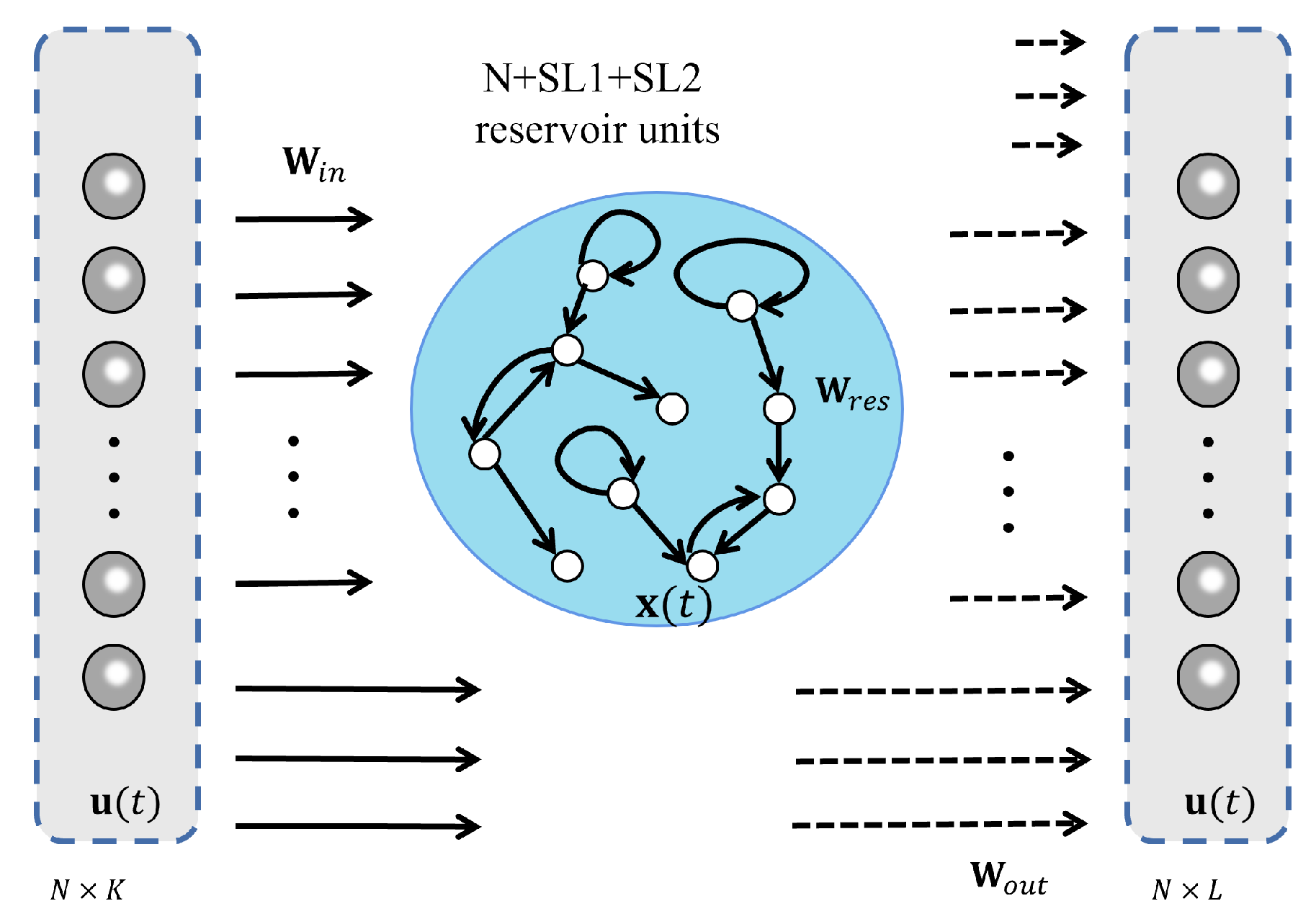
Figure 1 illustrates an ESN structure. An ESN architecture consists of three layers: (1) Input Layer: Receives external data and feeds them into the reservoir layer. (2) Reservoir Layer: This large layer contains interconnected neurons with fixed weights (a key ESN feature). These neurons process the input data through a complex nonlinear transformation and forward the result to the output layer. (3) Output Layer: A linear layer that maps the transformed data to the desired output.

The mathematical expression of ESN is

$$\begin{array}{c}{x}_t=\varphi \left[W_{in}{u}_t+W_{res}{x}_{t-1}\right]\hfill \\ y_t=W_{out}{x}_t\hfill \end{array}$$

(11)

where the input to the ESN at time step t is denoted by $u_t\in {\mathbb{R}}^n$, where n is the dimensionality of the input. The output of the network at time step t is denoted by $y_t\in {\mathbb{R}}^m$, where m is the dimensionality of the output. The state of the reservoir layer at time step t is provided by $\mathbf{x}\left(t\right)\in {\mathbb{R}}^N$. The ESN has a reservoir layer consisting of N neurons, $W_{in}\in {\mathbb{R}}^{N\times n}$ is the input weight matrix, $W_{res}\in {\mathbb{R}}^{N\times N}$ is the recurrent weight matrix, $W_{out}\in {\mathbb{R}}^{m\times N}$ is the output weight matrix, and $\varphi$ is an element-wise activation function.

The recurrent layer is

$$x_t=(1-\alpha )x_{t-1}+\alpha x_t$$

(12)

where $\alpha$ is the leaking rate.

The weights $W_{in}$ and $W_{res}$ are randomly initialized with fixed weights. The weights of the output layer $W_{out}$ are adjusted using the least squre algorithm

$$W_{out}={\left(X^{T}X+\beta I\right)}^{-1}X{Y}^T$$

(13)

where X is the matrix of reservoir states $x\left(t\right)$ for all time steps t, Y is the matrix of desired outputs $y_t$ for all time steps t, $\beta$ is a regularization parameter, and I is the identity matrix.

For time series modeling, Y is the target vector, and X is historical data. This approach greatly simplifies the training process and reduces the risk of overfitting since the complexity of the model is largely determined by the size and connectivity of the reservoir layer.

2.3. Echo State ARIMA Model (ES-ARIMA)

To address forecast lag, where predictions lag behind actual values, the AR and “I” models are commonly used, which are described in the above Equation (5). AR models can also correct other errors, like over- or under-prediction, by capturing trends, seasonality, and other patterns in the data through linear relationships between observations. Additionally, the error feature layer, inspired by the MA model in the above Equation (2), tackles the issue of random errors or noise in the time series data.

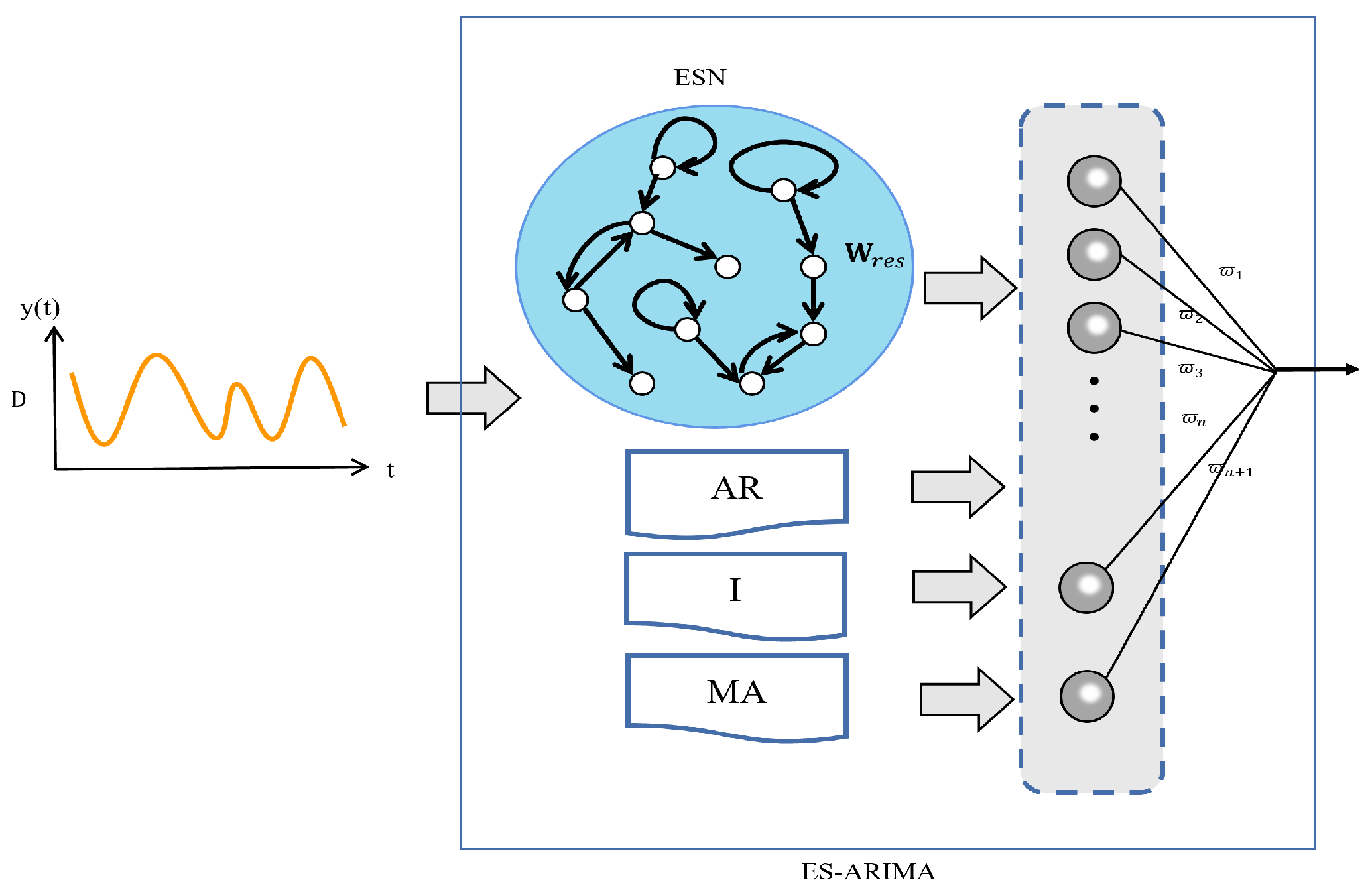
In this paper, we integrate the ARIMA model into the recurrent part of the ESN, resulting in the ES-ARIMA model. Figure 2 illustrates its structure. ES-ARIMA combines an ESN with an ARIMA model. ES-ARIMA has two main blocks:

• ESN section: This section includes elements similar to the ESN diagram, such as reservoir neurons, input layer, and output layer. It also shows connections between these elements.
• ARIMA section: This section depicts elements representing the ARIMA model’s components, such as Autoregressive (AR) and Moving Average (MA) components, with arrows indicating the flow of information.

The ES-ARIMA model includes three parts: linear features ${\Omega }_{lin},$ error features ${\Omega }_{error}$, and nonlinear features ${\Omega }_{Nonlinear}.$ They are

• The linear features ${\Omega }_{lin,t}$ at time step t are composed of observations from the input vector $u_t;$ in Figure 1, the input is previous time series $y_{t-1}$ in dataset D. At the current time t and previous time $t-s$,

  $${\Omega }_{lin,t}=U_t\cup U_{t-s}\cdots \cup U_{t-(k-1)s}$$

  (14)

  where $U_t={[u_{1,t},\cdots ,u_{l,t}]}^T$ is a l-dimensional vector, ${\Omega }_{lin,t}$ has $l\times k$ matrix, and s is the number of skipped steps between consecutive observations. ${\Omega }_{lin,t}$ is used in the ARIMA model in Figure 2.
• The error features ${\Omega }_{error}$ is

  $${\Omega }_{error,t}={ϵ}_t\cup {ϵ}_{t-1}\cup \cdots \cup {ϵ}_{t-q}$$

  (15)

  where $ϵ$ and q are defined in (2). It is the MA model in Figure 1. In time series forecasting, random errors can have a significant impact on the accuracy of predictions, causing them to deviate from the actual values. By modeling the noises as in (15), the  accuracy of predictions can be improved. Additionally, MA models can help the ES-ARIMA model to identify the short-term fluctuations in the data.
• The nonlinear feature ${\Omega }_{Nonlinear}$ is obtained from the echo state network,

  $${\Omega }_{nonlinear}=x_1\cup \cdots \cup x_n$$

  (16)

  where $x_i$ is defined in (12). Obviously, ${\Omega }_{Nonlinear}$ is the state vector of classical ESN.

The state of ES-ARIMA model $X_t$ is

$$X_t=c\cup {\Omega }_{lin,t}\cup {\Omega }_{error,t}\cup {\Omega }_{Nonlinear}$$

(17)

where c is a constant.

The output signal of ES-ARIMA ${\widehat{y}}_t$ can be expressed as

$${\widehat{y}}_t={\overline{W}}_{out}\times X_t$$

(18)

The training of the ES-ARIMA is the same as ARIMA (10) and ESN (13), and the parameter vector $W_{out}$ is the combination of $\theta$ defined in (6) and $W_{out}$ defined in (11), i.e.,

$${\overline{W}}_{out}=\left[W_{out},\theta \right]$$

(19)

ES-ARIMA models, like many other statistical models, are susceptible to overfitting. We use the following method to prevent overfitting:

• Information Criteria: When choosing the ARIMA order $(p,d,q)$, rely on information criteria like AIC or BIC instead of simply picking the model with the lowest in-sample error on the training data. These criteria penalize models for complexity, favoring simpler models that perform well on unseen data.
• Limit Model Complexity: Avoid excessively high orders $(p,d,q)$ for the ES-ARIMA model. Start with a simpler model and increase complexity only if the information criteria or diagnostics on the residuals suggest a need for more parameters.

3. Training of ES-ARIMA Model

3.1. Frequency Decomposition

Time series forecasting involves predicting the future values of a series over time, essentially anticipating its behavior several steps ahead. Frequency decomposition is a valuable technique that separates a time series into its constituent frequencies. This decomposition reveals hidden patterns within the data, which are particularly beneficial for prediction tasks.

High-frequency components capture short-term fluctuations, while low-frequency components reflect long-term trends. By decomposing the signal, the neural network can effectively distinguish between these timescales. It can then focus on the relevant component, whether it is the underlying trend (low frequency) or the short-term volatility (high frequency). For long-term forecasts, the model prioritizes the information contained in the low-frequency components.

Predicting the original time series $y_t$ directly with models like ESN and ARIMA can be challenging. However, decomposing the signal into its constituent frequencies makes each component more suitable for specific prediction methods

$$G\left(y\right)=\frac{y+a}{1+ay}$$

(20)

where $\left|a\right|\le 1$, it corresponds to the cutoff frequencies, which can be obtained by applying the more general lowpass-to-highpass transformation. or short-term predictions. If long-term forecasting is required, the weight of low frequency will be higher than high frequency.

Low-frequency components are well-suited for linear prediction using ARIMA, while high-frequency components benefit from nonlinear prediction methods like ESN:

$$X_t=F\times X_t+tanh\left[W_{in}{\Omega }_{lin,t}+W{X}_{t-1}\right]$$

(21)

Here, $F\in {\mathbb{R}}^{1\times l}$ represents the forget weight, allowing the network to combine high- and low-frequency signals at different times.

Low-frequency signals facilitate long-term memory in ESN. By incorporating the ARIMA model’s weights as the forgetting rate, the network can selectively choose relevant information from the ESN, improving its ability to adapt to changes over time. This essentially allows the model to “forget” outdated information and focus on the most relevant data for prediction.

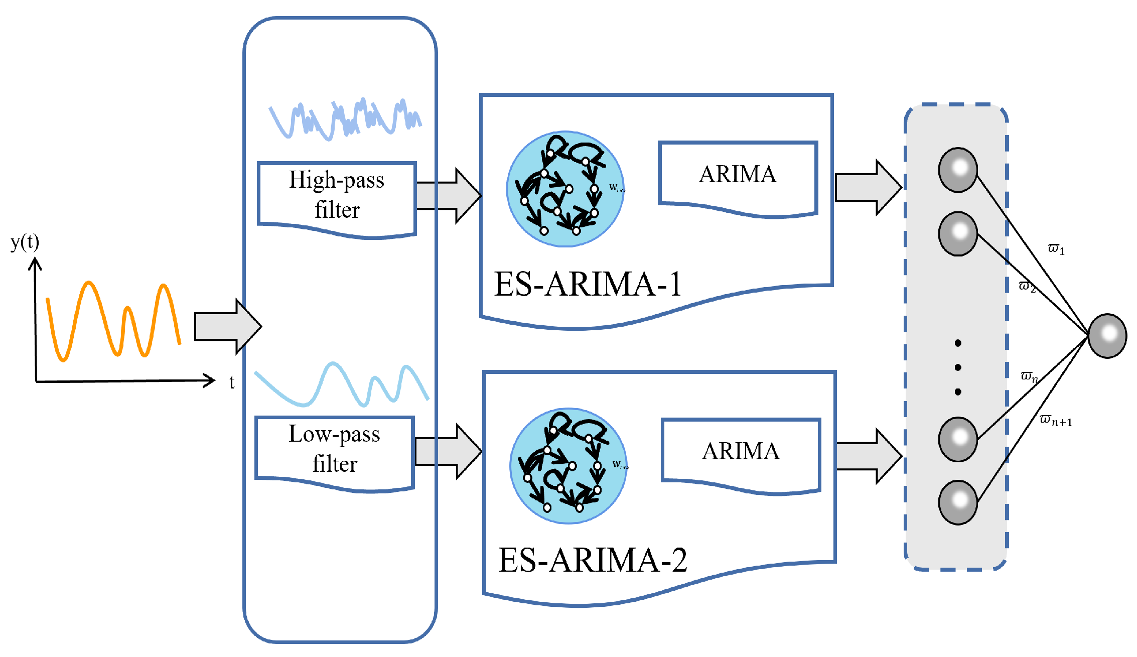
As shown in Figure 3, high-frequency signals capture fine details, while low-frequency signals provide the overall form and structure. We utilize another neural network to fuse the high-frequency and low-frequency components obtained after decomposition:

$$\begin{array}{c}{\widehat{y}}_h=ES\_ARIM{A}_h\left(y_h\right)\\ {\widehat{y}}_l=ES\_ARIM{A}_l\left(y_l\right)\end{array}$$

(22)

where $y_h$ is high-frequency signal, $y_l$ is low-frequency signal, where ${\widehat{y}}_{h,t}$ and ${\widehat{y}}_{l,t}$ are the outputs of the low- and high-frequency ES-ARIMA models, respectively.

Finally, a two-layer Multilayer Perceptron (MLP) combines ${\widehat{y}}_{h,t}$ and ${\widehat{y}}_{l,t}$:

$${\widehat{y}}_{t+1}=W_f\sigma \left(\left[V_l{\widehat{y}}_{l,t}+V_h{\widehat{y}}_{h,t}\right]\right)$$

(23)

where $V_h,$$V_h$, and $W_f$ are the weights, ${\widehat{y}}_{t+1}$ is the final prediction, and $\sigma$ is a nonlinear activation function.

3.2. Transfer Learning

Missing values in time series data can be handled in two ways: dropping them or imputing them (replacing them with estimated values). While methods like linear interpolation, spline interpolation, and k-nearest neighbors exist for imputation, they may not work well for non-randomly distributed missing values. Recent research suggests that deep learning methods like Long Short-Term Memory (LSTM) networks can handle such scenarios more effectively.

Many existing prediction methods require sufficient and evenly distributed data. Transfer learning can be used to address this challenge by transferring knowledge from one time series (e.g., with complete data) to another (e.g., with missing values). This can improve the accuracy of machine learning algorithms for time series data with missing values.

Traditional ARIMA models struggle when dealing with uncertainties in training data, such as missing values. Let us assume the training data ${\Lambda }_a$ has missing values, while datasets ${\Lambda }_b$ and ${\Lambda }_c$ share similar distributions with ${\Lambda }_a$. Our goal is to recover ${\Lambda }_a$ using data from ${\Lambda }_b$ and ${\Lambda }_c$. If a relationship $\Omega$ exists between ${\Lambda }_b$ and ${\Lambda }_c$, we can express ${\Lambda }_a$ as a function of them ${\Lambda }_a=F[{\Lambda }_b,{\Lambda }_c]$. This section proposes a transfer learning approach where the ESN-ARIMA_a model can utilize the combined dataset $\Lambda ={\Lambda }_a\cup {\Lambda }_b\cup {\Lambda }_c$.

For an ESN-ARIMA_a model, the training objective is to minimize both the training error and the number of parameters, as shown in the following equation:

$$J_a=\underset{W^a}{min}\left\{\lambda {∥W^a∥}^2+{∥x_t^a{W}^a-y_a^{target}∥}^2\right\}$$

(24)

where $W^a$ and $x_t^a$ are the weight and the state of the ESN-ARIMA model, $y_a^{target}$ is the desired value.

For an ESN-ARIMA_a model, the training objective is to minimize both training error and parameters, as follows: where $1>\lambda >0,$ it is the regularization parameter, $Y_a^{target}\in {\Lambda }_a.$

When there are missing values in ${\Lambda }_a,$ we use ${\Lambda }_b$ to help us to improve the model ES-ARIMA_a.

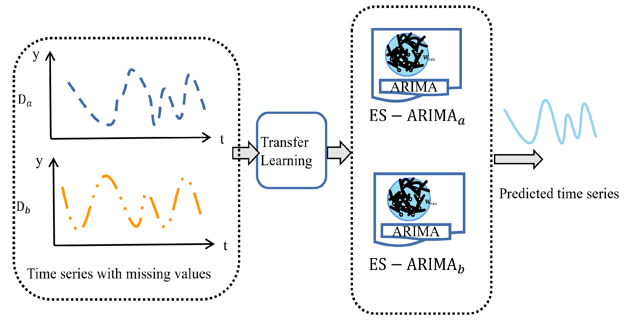
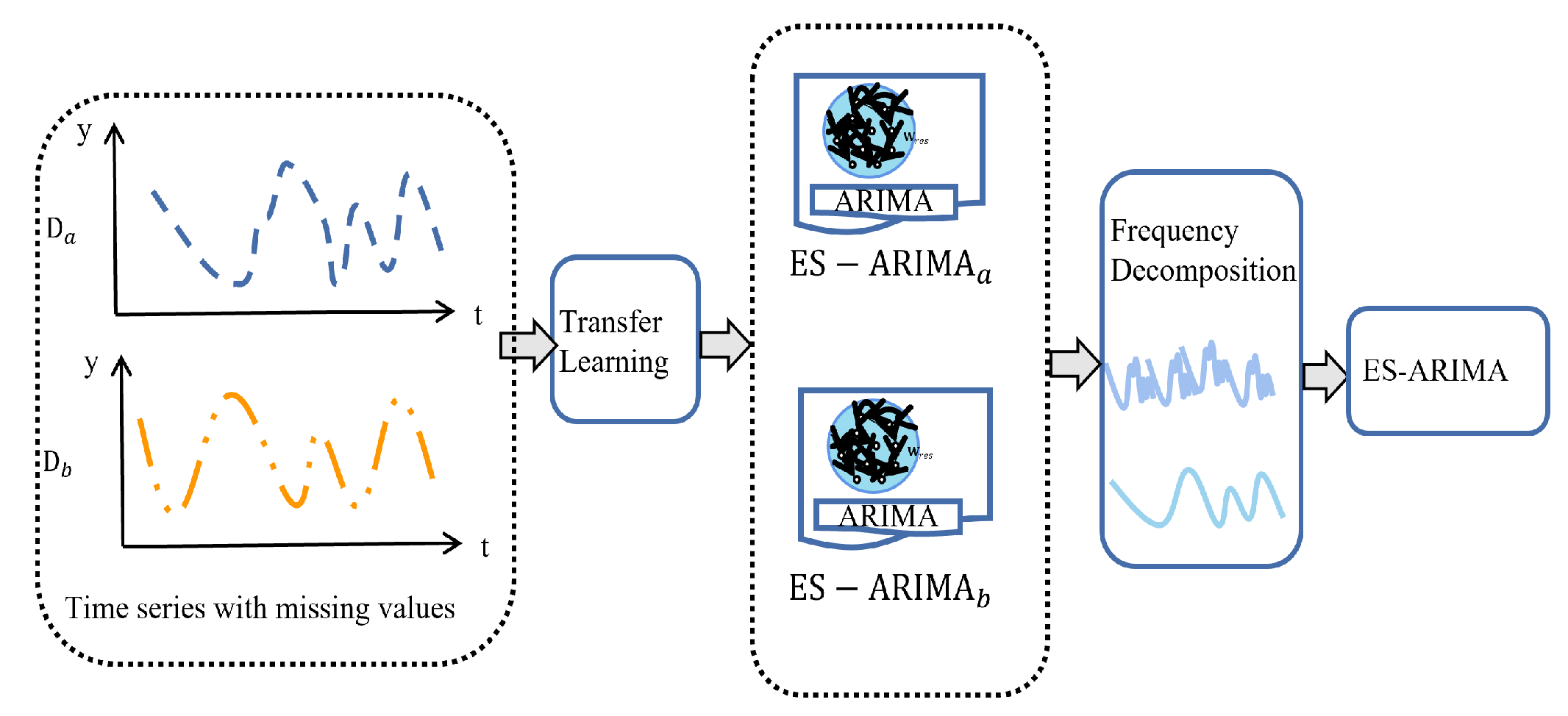
This source task ${\Lambda }_b$ uses a pre-trained Echo State Network (ESN) on a different but related time series forecasting problem of ${\Lambda }_a$. The pre-trained ESN captures some general knowledge in ${\Lambda }_b$ that can be beneficial for the target task ${\Lambda }_a$. The knowledge transfering from the source task ${\Lambda }_b$ to the target task ${\Lambda }_a$ involves using the weights or activations learned by the pre-trained ESN as a starting point for training the ESN component within the ES-ARIMA model. This transfer learning is shown in Figure 4.

The training index is defined as

$$J_{ab}=\underset{W^a,W^b,{\xi }_a,{\xi }_b}{min}\left\{\begin{array}{c}\frac{1}{2}{∥W^b∥}^2\\ +\frac{C_a}{2}{\sum }_{i=1}^{l_a}{∥{\xi }_a∥}^2+\frac{C_b}{2}{\sum }_{j=1}^{l_b}{∥{\xi }_b∥}^2\end{array}\right\}$$

(25)

where ${\xi }_a=x_t^a{W}^a-Y_a^{target},{\xi }_b=x_t^b{W}^b-Y_b^{target}$, $C_a$ and $C_b$ are positive constants: they are the penalty coefficients on the prediction error from source and target domain, and $l_a$ and $l_b$ are the lengths of datasets ${\Lambda }_a$ and ${\Lambda }_b$. $W^b$ denotes the output weight vector of the domain ${\Lambda }_b$; $Y_b^{target}$ is the target dataset $B.$ From (24), we obtain the local solution $W^a$. From (25), we will learn $W^b$ using all data from the source domain ${\Lambda }_b$ by leveraging a limited number.

For ES-ARIMA model, $X_t^a\in R^{1\times N}$, ${\xi }_a\in R^{1\times l_a}$, $Y_t^a\in R^{1\times l_a}$ denote the states of reservoir, the prediction error, and the target value in the domain ${\Lambda }_a$. $X_t^b\in R^{1\times N}$, ${\xi }_b\in R^{1\times l_b}$, $Y_t^b\in R^{1\times l_b}$ denote the states of reservoir, the prediction error, and the target value in the domain ${\Lambda }_b$. The corresponding Lagrangian problem of (25) is

$$\begin{array}{c}L(W^b,{\xi }_a,{\xi }_b,{\alpha }_a,{\alpha }_b)=\frac{1}{2}{∥W^b∥}^2+\frac{C_a}{2}{\sum }_{i=1}^{l_a}{∥{\xi }_a∥}^2\hfill \\ +\frac{C_b}{2}{\sum }_{j=1}^{l_b}{∥{\xi }_b∥}^2-{\alpha }_a(X_i^a{W}^b-Y^a+{\xi }_a)\hfill \\ -{\alpha }_b(X^b{W}^b-Y^b+{\xi }_b)\hfill \end{array}$$

(26)

where ${\alpha }_a$ and ${\alpha }_b$ are Lagrangian multiplier vectors. The  problem (26) can be solved by

$$\left\{\begin{array}{c}\frac{\partial L}{\partial W^b}=0\to W^b=x_t^a{\alpha }_a+x_t^b{\alpha }_b\hfill \\ \frac{\partial L}{\partial {\xi }_a}=0\to {\alpha }_a=C_a{\xi }_a^T\hfill \\ \frac{\partial L}{\partial {\xi }_b}=0\to {\alpha }_b=C_b{\xi }_b^T\hfill \\ \frac{\partial L}{\partial {\alpha }_a}=0\to x_t^a{W}^b-Y_a+{\xi }_a=0\hfill \\ \frac{\partial L}{\partial {\alpha }_b}=0\to x_t^b{W}^b-Y_b+{\xi }_b=0\hfill \end{array}\right.$$

(27)

where $x_t^a$ and $x_t^b$ are the output matrix of reservoir layer with respect to the data from target domain ${\Lambda }_a$ and source domain ${\Lambda }_b$, respectively.

The solution of (27) is

$$W^b={(I+C_b{x}_t^b{x}_t^b+C_a{x}_t^a{x}_t^a)}^{-1}(C_b{x}_t^b{Y}_b+C_a{x}_t^a{Y}_a)$$

(28)

Calculating the matrix inverse, as shown in Equation (28), can be computationally expensive and resource-intensive, especially for real-time applications and large matrices. This high demand for computational power and memory limits its practical use. To address this challenge, this paper proposes a novel recursive method for finding the inverse. This method offers several benefits, including

• Fast convergence: It reaches the solution quickly, making it suitable for real-time applications.
• Low computational complexity: It requires fewer calculations compared to traditional methods, reducing computational burden.
• Improved numerical stability: It produces more accurate results, especially when dealing with ill-conditioned matrices.

To implement the recursive method, we require the use of the following matrix inverse lemma:

$${(A+BCD)}^{-1}=A^{-1}-A^{-1}B{(C^{-1}+D{A}^{-1}B)}^{-1}D{A}^{-1}$$

(29)

where $A\in R^{n\times n}$, $C\in R^{m\ast m}$, $B\in R^{n\times m}$, $D\in R^{m\times n}$. We define $R_t^{-1}=C_a{x}_t^a{x}_t^a+C_b{x}_t^b{x}_t^b+I$, $Z_t=C_b{x}_t^b{Y}_b+C_a{x}_t^a{Y}_a$, $W^b=R_t^{-1}{Z}_t$. Then,

$$\begin{array}{c}{R}_t^{-1}=C_a{x}_t^a{x}_t^a+C_b{x}_t^b{x}_t^b+I\hfill \\ =R_{t-1}^{-1}+C_a{x}_t^{aT}{x}_t^a+C_b{x}_t^{bT}{x}_t^b+I\hfill \\ =R_{t-1}^{-1}+\left[\begin{array}{cc}{C}_a& C_b\end{array}\right]\left[\begin{array}{c}{x}_t^a\\ x_t^b\end{array}\right]\left[\begin{array}{cc}{x}_t^a& x_t^b\end{array}\right]+I\hfill \end{array}$$

(30)

Then, we can define $A=R_t^{-1}$, $B=R_{t-1}^{-1}$, $C={[x_t^a\left(t\right),x_t^b\left(t\right)]}^T$, $D=[C_a,C_b]$ using (29), (30) is

$$\begin{array}{c}{R}_t^{-1}=R_{t-1}^{-1}+R_{t-1}^{-1}C{([C_a,C_b]+C^T{R}_{t-1}^{-1}C)}^{-1}{C}^T{R}_{t-1}^{-1}+I\hfill \\ =R_{t-1}^{-1}+\frac{R_{t-1}^{-1}C{C}^T{R}_{t-1}^{-1}}{[C_a,C_b]+C^T{R}_{t-1}^{-1}C}+I\hfill \\ =R_{t-1}^{-1}+\frac{R_{t-1}^{-1}{[x_t^a,x_t^b]}^T[x_t^a,x_t^b]R_{t-1}^{-1}}{[C_a,C_b]+[x_t^a,x_t^b]R_{t-1}^{-1}{[x_t^a,x_t^b]}^T}+I\hfill \end{array}$$

(31)

If $R_t^{-1}=P_t$, then $P_t=P_{t-1}+\frac{P_{t-1}C{C}^T{P}_{t-1}}{I+C^T{P}_{t-1}C}.$ We define $K_t=\frac{P_{t-1}C}{I+C^T{R}_{t-1}^{-1}C}$ as gain vectors, and then

$$\begin{array}{cc}\hfill P_t& =P_{t-1}+K_t{C}^T{P}_{t-1}+I\hfill \\ \hfill & =P_{t-1}+K_t\left[x_t^a,x_t^b\right]P_{t-1}+I\hfill \end{array}$$

(32)

So, the output weight updates can be performed using

$$\begin{array}{c}{W}_t=P_t{Z}_t=P_t[Z_{t-1}+x_t^a{y}_t^a+x_t^b{y}_t^b]\hfill \\ =[P_{t-1}+K_t{C}^T{P}_{t-1}]Z_{t-1}+P_t{x}_t^a{y}_n^a+P_t{x}_t^b{y}_t^b\hfill \\ =W_{t-1}-K_t(C^T{W}_{t-1}-y_t^a-y_t^b)\hfill \\ =W_{t-1}-K_t(e_a+e_b)\hfill \end{array}$$

(33)

where the error $e_a=x_t^a{W}_{t-1}-Y_a$ and $e_a=x_t^b{W}_{t-1}-Y_b$ can be easily computed. The scheme of the long-term prediction of time series with missing values using echo state ARIMA model is shown in Figure 5.

For implementation, the ES-ARIMA algorithm is summarized in Algorithm 1.

Algorithm 1 ARMA-ESN

1: The inputs are the time series $y_a\left(k\right),y_b\left(k\right)$ in datasets ${\Lambda }_a,{\Lambda }_b$. ${\Lambda }_a$ is the target domain. ${\Lambda }_b$ is the source domain. 2: Initialize two ESN networks, with N hidden neurons, random input weights $W_{in}$, and reservoir W for both target and source domains. 3: Use algorithm RLS to obtain AR model weights as ESN forgetting rate. 4: Calculate the hidden matrix $X^a$ and $X^b$ according to (21). 5: Compute the output weights $W_{out}$ using (33). 6: Return the output weights $W_{out}$ and predicted output $Y_a$. 7: The outputs are predicted output $y_a(k+m)$ and $y_b(k+m)$.

Here, several remarks on the proposed method are presented:

• While the proposed method offers significant advantages in handling missing data and improving forecasting accuracy, it is important to acknowledge the potential increase in computational complexity compared to simpler approaches. This is particularly relevant for large-scale datasets.
• The potential increase in computational cost needs to be weighed against the significant benefits gained in terms of accuracy and robustness, especially for applications where high-fidelity wind speed prediction is crucial. Further research can explore optimization techniques to further enhance the scalability of the proposed method for even larger datasets.
• The effectiveness of the method can be influenced by the quality of the data, particularly the extent and pattern of missing data. High percentage of missing values, especially if randomly distributed, could hinder the model’s ability to learn the underlying patterns in the data. One ideal approach might involve a combination of the method with data preprocessing techniques specifically tailored to the characteristics of the missing data.
• While the proposed model offers significant improvements in accuracy by combining multiple techniques (ESN, ARIMA, frequency decomposition, and transfer learning), this complexity might come at the cost of interpretability. Understanding the exact contributions of each component to the final prediction can be challenging. Further research can explore additional methods for enhancing interpretability, such as visualization techniques or model-agnostic interpretable machine learning approaches. This will enable deeper understanding of the internal workings of the model and potentially lead to further improvements in its performance.
• We acknowledge that the proposed method’s success is tied to the availability of sufficient historical data. However, the framework incorporates techniques that can use even smaller datasets effectively. Additionally, the transfer learning component allows the model to potentially benefit from knowledge learned from related domains, even if the target domain has limited data. While the ideal scenario involves abundant high-quality data, our approach offers advantages over existing methods by achieving a good baseline level of accuracy and capturing essential trends even with limited data availability.

4. Applications

To demonstrate the effectiveness of our Echo State ARIMA (ES-ARIMA) model for handling such data, we apply the proposed approach to real-world wind speed systems.

In recent decades, wind speed has emerged as a key solution to address the challenges of climate change and the growing demand for electricity. Its cleaner and more sustainable nature has propelled it to become one of the most important clean energy sources globally [32,33,34]. However, the efficiency of wind power generation is hampered by the inherent variability and uncertainty of wind speed and direction [35].

Wind speed forecasting, a crucial application of time series prediction, plays a vital role in mitigating these challenges. The existing prediction models can be broadly categorized into four types: physics-based, statistical, neural network, and fusion models. Each type is suitable for different time scales, with statistical models commonly employed for short-term forecasting and physical models favored for long-term predictions [20]. These time scales range from very short-term (seconds to 30 min) to very long-term (beyond 72 h).

This study utilizes three datasets from diverse geographical regions: Kaggle [36], Germany [37], and California [38]. We employ $75\%$ of each dataset for training multiple ARIMA models and the remaining $25\%$ for testing. These datasets contain 18,000 records. We used the first 15,000 records for training the model and the remaining 3000 records for testing.

The dataset details are (1) Time Period: the date range covered by the data is one year. (2) Features: the datasets include wind speed, wind direction, temperature, pressure, and humidity. (3) Target variable: wind speed. (4) Time Step: hourly. We aggregate these hourly values to create a daily time series. (5) Missing Values: approximately $30\%.$

• Kaggle Dataset: It contains hourly values from 7 wind farms spanning from July 2009 to June 2012. We use data from the first wind farm between 1 July 2009 and 31 December 2010.
• California Dataset: It records hourly energy production from 5 wind farms, including geothermal, biomass, biogas, mini-hydraulic, total wind, solar photovoltaic, and solar thermal. We use data from 1 September 2011 to 31 August 2012.
• Germany Dataset: This dataset encompasses data from four wind farms: Tennet, 50 Hertz, TransnetBW, and Amprion. The data are from 1 January 2011 to 31 December 2011.

We use the following min–max normalization to scale the data to a similar range, leading to faster training and convergence of neural networks,

$$y_{norm}\left(i\right)=\frac{y_i-min\left(y\right)}{max\left(y\right)-min\left(y\right)}$$

(34)

where $y_i$ is each datum of the time series, $min\left(y\right)$ is the minimum of the data y, and $max\left(y\right)$ is the maximum of the data y.

For long-term prediction of time series,

$$y_{t+m}^{\ast }=f\left(y_{t-1}^{\ast },y_{t-2}^{\ast },\cdots \right)$$

(35)

where $m\ge 1,$ in this paper, we select $m=2,$ i.e., for daily records of wind speed. We consider 48 h forecasts in the simulations because

• While short-term forecasts are most valuable for real-time operations, including 48 h forecasts, this showcases the proposed method’s ability to handle a wider range of prediction horizons.
• Research suggests that incorporating information from longer time frames can sometimes improve the accuracy of shorter-term forecasts. By including 48 h data in the training process, we might be capturing underlying patterns that benefit the overall performance, even for the crucial short-term predictions.

The model is

$$y_{t+m}=ARIMA\left(y_{t-1},y_{t-2},\cdots \right)$$

(36)

Time series forecasting is

$$y_{t+m+1}^{\ast }\approx y_{t+m+1}=ARIMA\left(y_t^{\ast },y_{t-1}^{\ast },\cdots \right)$$

(37)

Wind speed plays a critical role in determining electricity generation by wind turbines. However, wind speed datasets often exhibit limitations. High wind speeds, crucial for accurate forecasting, occur only for a small fraction of the year (around $0.1\%$). This imbalance can negatively impact prediction accuracy for high wind speeds compared to regular wind speeds.

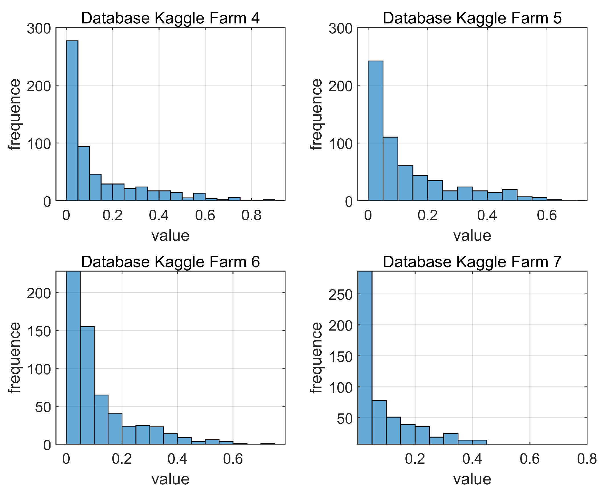
To demonstrate the effectiveness of our transfer learning approach, we utilize the Kaggle dataset. It contains hourly wind speed data from 7 wind farms between July 2009 and June 2012. Despite the missing data, the wind speed data across the different farms exhibit substantial similarity due to their geographic proximity. This similarity is ideal for applying transfer learning techniques. These techniques can leverage knowledge gained from one dataset (source domain) to improve predictions for another (target domain). The histogram of wind speed data from different farms is illustrated in Figure 6.

The equation for the ES-ARIMA model is shown in (17). To determine the appropriate ARIMA model structure, we need to analyze the stationarity of the data and obtain the value of d. We use the Augmented Dickey–Fuller (ADF) test [39] for stationarity analysis. The results are presented in

Table 1. Dickey–Fuller testing results of the datasets.

Serie	ADF Statistic	p-Value	1%	5%	10%	H0	d
Kaggle1	−2.2	0.2	−3.4	−2.9	−2.6	not stationary	0
Kaggle2	−7.9	0.041	−3.4	−2.9	−2.61	stationary	1
Germany	−2.9	0.045	−3.4	−2.8	−2.5	stationary	0
California1	−1.2	0.66	−3.4	−2.8	−2.5	not stationary	0
California2	−9.7	0.086	−3.4	−2.8	−2.5	stationary	1

.

Critical values of $1\%$, $5\%$, and $10\%$ are used for the ADF hypothesis test. If the hypothesis is accepted, the ARIMA model contains a unit root, indicating non-stationarity. For the Kaggle dataset, the initial test with zero differentiation produces a value of $-2.153$. This value is less than all critical values, indicating the time series needs differencing. After one differentiation, the hypothesis is accepted, making the Kaggle set stationary with $d=1$.

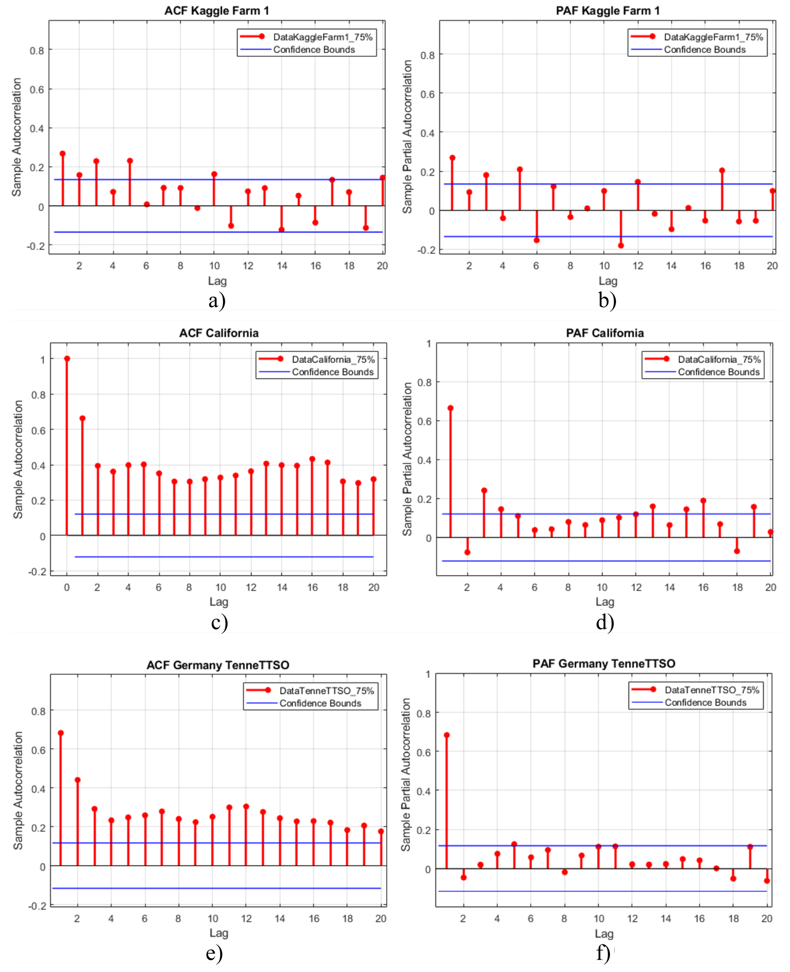
ACF (Autocorrelation Function) and PAF (Partial Autocorrelation Function) are crucial tools for selecting the appropriate ARIMA model order (p, d, q). By analyzing their patterns, we can identify and address autocorrelations in our time series data, leading to a more accurate model. Figure 7 shows the ACF/PAF plots for the three datasets.

Table 2. ARIMA model parameters obtained with the tests of ACF, PAF, and the augmented Dickey–Fuller test.

Serie	p	d	q
Germany	1,2	0	1,2,3,4,5
California	1,2,3,4,5,6	1	0
Kaggle	1,2	1	1,2,3

displays the ARIMA parameters obtained from ACF/PAF analysis and the ADF test. So, the optimal ARIMA models for the datasets are Kaggle—ARIMA(1,1,2), Germany—ARIMA(1,0,4), and California—ARIMA(0,1,2).

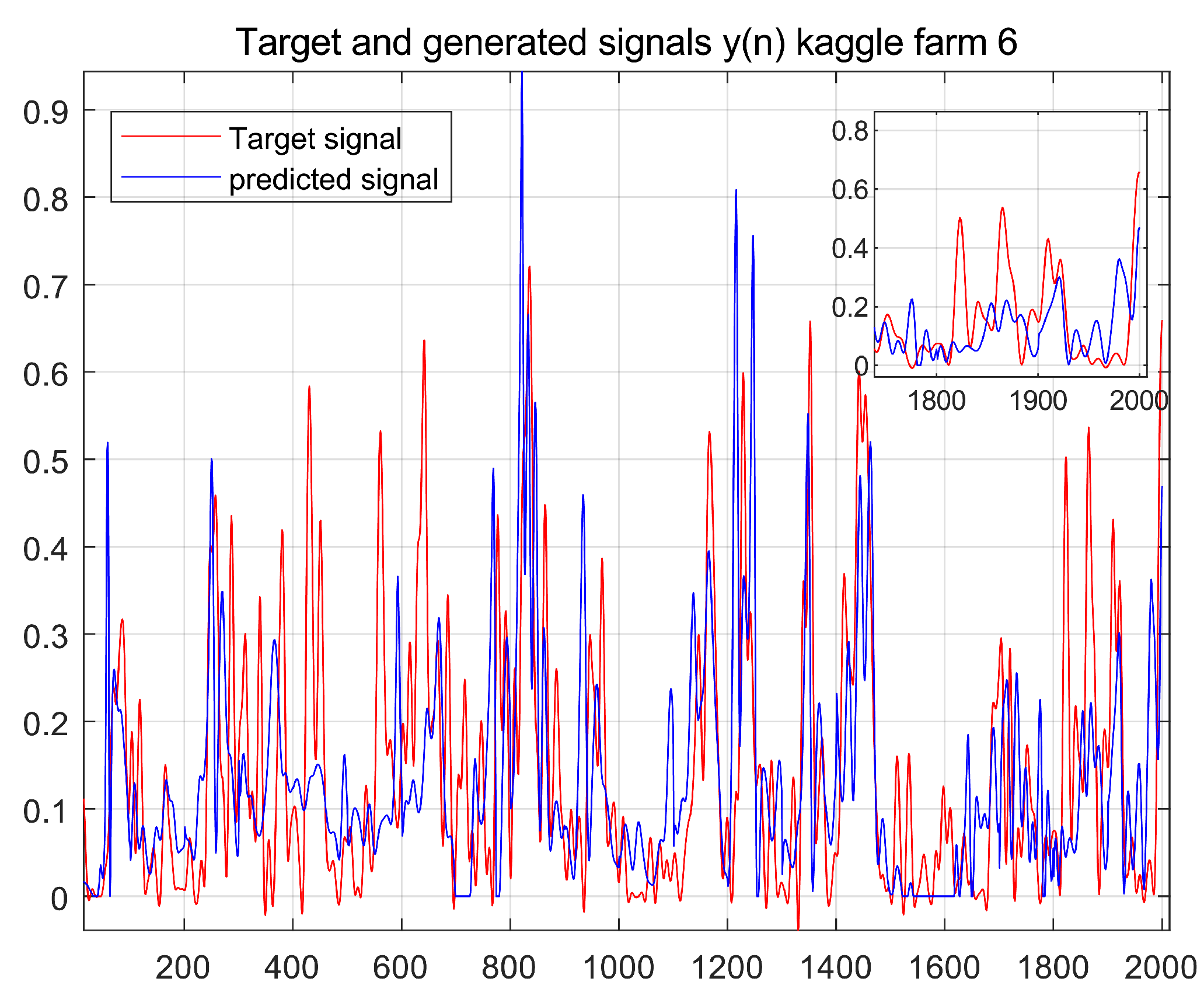
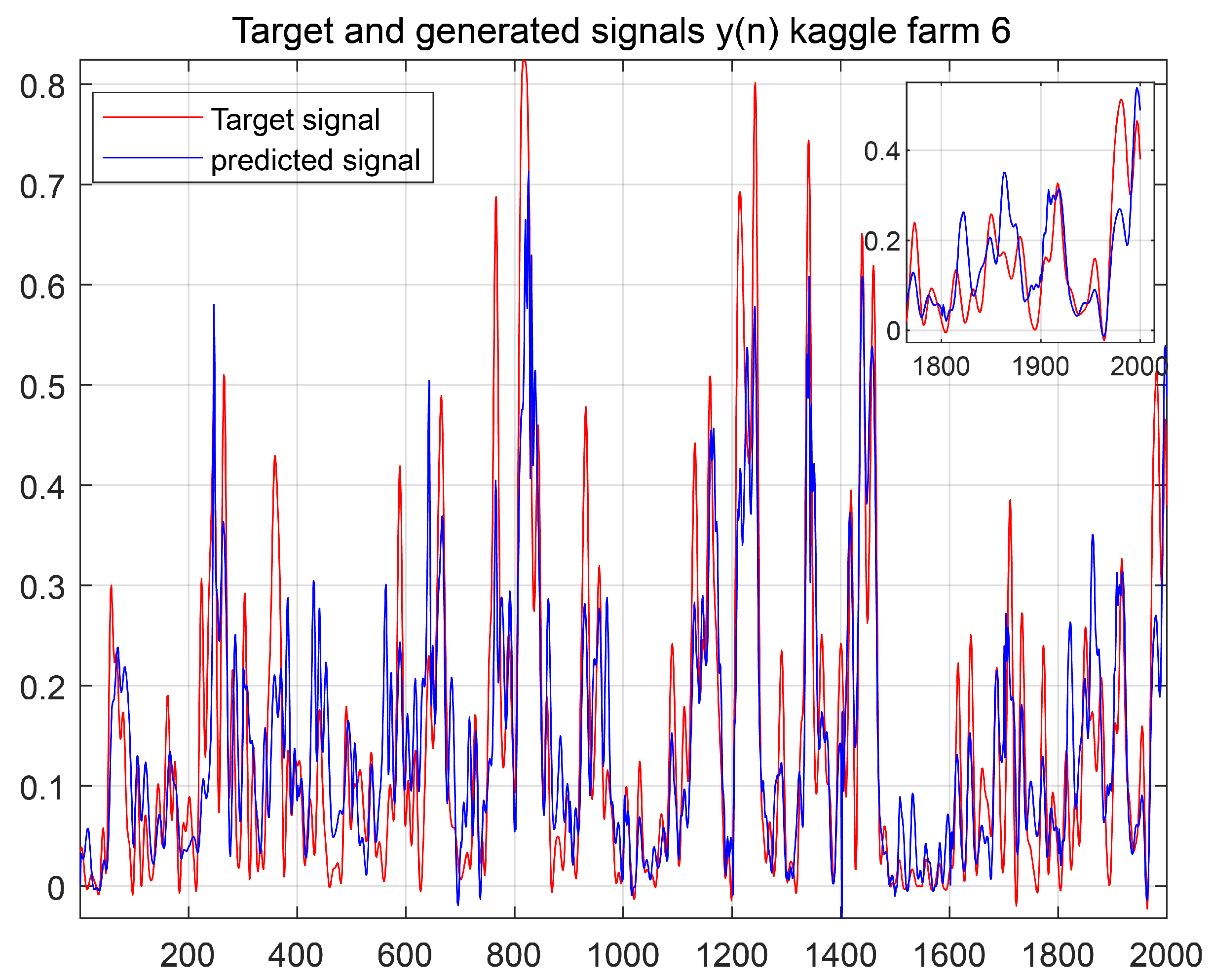
The prediction results using the ES-ARIMA model are shown in Figure 8.

In frequency decomposition, the transfer function of the filters is

$$G\left(y\right)=\frac{y+0.17}{1+0.17y}$$

(38)

where $0.17$ corresponds to the cutoff frequencies.

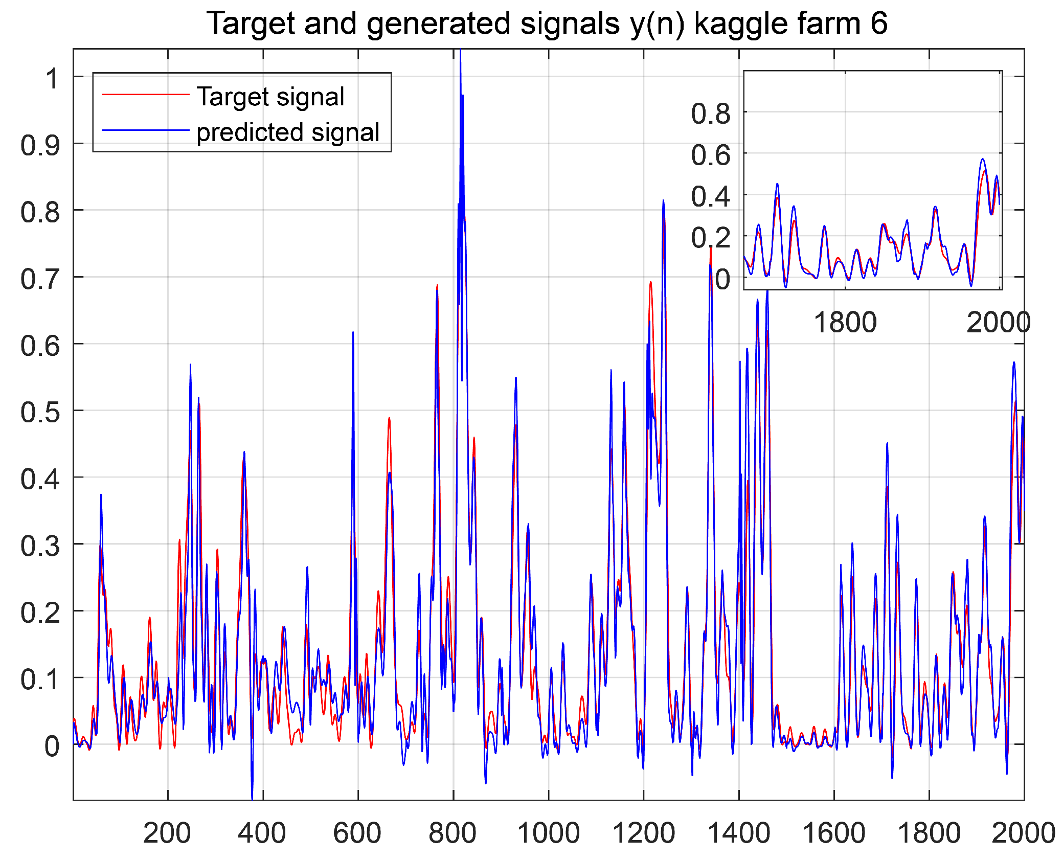
Figure 9 depicts the prediction results with frequency decomposition and ES-ARIMA. While these results are better than using only ES-ARIMA, missing data still affect the accuracy.

We aim to enhance prediction accuracy by leveraging transfer learning. This technique allows the model to identify patterns and relationships common across different datasets, leading to more accurate and robust predictions. Our objective is to forecast data in Farm 6 by utilizing information from other farms (source domain).

As shown in Figure 10, transfer learning generally delivers favorable results when source and target domains exhibit high similarity. However, low similarity can lead to lower performance, as illustrated in Figure 9.

Despite the limitations in this case, transfer learning still outperforms directly supplementing Farm 6 data with data from Farm 5. This highlights the potential of transfer learning to improve predictions even with low similarity between source and target domains. By utilizing knowledge from related datasets, transfer learning can help to mitigate the impact of missing data in the target domain.

Comparisons

ARIMA Models vs. Neural Networks:

ARIMA Models: These models are widely used for time series forecasting and excel at identifying patterns and trends in historical data. However, they may struggle with complex relationships or nonlinear data.

Neural Networks: These powerful machine learning techniques can learn complex patterns and relationships, even in nonlinear data. They often outperform ARIMA models in terms of accuracy but require more computational power and data for training.

Comparison with Other Forecasting Methods:

We compared our ES-ARIMA model with several classical methods:

• Multilayer Perceptron (MLP): A type of artificial neural network.
• Classical Echo State Network (ESN): A type of recurrent neural network.
• ARIMA: The standard ARIMA model.
• T-ARIMA: ARIMA with classical transfer learning.
• ARIMA: classical ARIMA model

Evaluation Metrics:

The following metrics were used to compare forecasting errors:

$$\begin{array}{c}MAE=\frac{{\sum }_i^n\left|y_i^{\ast }-y_i\right|}{n}\hfill \\ SMAPE=\frac{1}{n}{\sum }_i^n\frac{\left|y_i^{\ast }-y_i\right|}{\left(y_i^{\ast }+y_i\right)/2}\hfill \\ RMSE=\sqrt{\frac{{\sum }_i^n{\left(y_i^{\ast }-y_i\right)}^2}{n}}\hfill \\ R^2=1-\frac{{\sum }_i^n{\left(y_i^{\ast }-y_i\right)}^2}{{\sum }_i^n{\left(y_i-\overline{y}\right)}^2},\overline{y}=\frac{1}{n}{\sum }_i^n{y}_i\hfill \end{array}$$

(39)

where Mean Absolute Error (MAE): Average absolute difference between predicted and actual values. Symmetric Mean Absolute Percentage Error (SMAPE): Error metric less sensitive to outliers than other measures. Root Mean Squared Error (RMSE): Square root of the average squared difference between predicted and actual values. R-squared ($R^2$): Proportion of variance in the predicted values that can be explained by the independent variable (closer to 1 indicates better fit). However, high $R^2$ could be overfitting the training data.

Results and Discussion:

Table 3. Comparison of forecasting errors with California data.

Models	MAE	SMAPE	RMSE	R-Squared
MLP	1.23	0.42	4.84	0.82
ESN	2.46	1.63	5.37	0.79
T-ARIMA	1.67	0.87	2.26	0.89
ARIMA	1.92	1.21	3.65	0.83
ES-ARIMA	0.61	0.07	1.26	0.93

,

Table 4. Comparison of forecasting errors with Germany data.

Models	MAE	SMAPE	RMSE	R-Squared
MLP	0.26	0.72	0.39	0.91
ESN	0.487	0.73	0.763	0.85
T-ARIMA	0.73	0.58	0.81	0.81
ARIMA	0.82	0.71	0.57	0.89
ES-ARIMA	0.073	0.14	0.069	0.95

and

Table 5. Comparison of forecasting errors with Kaggle data.

Models	MAE	SMAPE	RMSE	R-Squared
MLP	1.82	0.95	3.78	0.83
ESN	1.45	1.64	2.97	0.87
T-ARIMA	1.82	0.92	2.93	0.88
ARIMA	1.51	1.14	2.87	0.92
ES-ARIMA	1.24	0.26	2.73	0.91

present the comparison results for the three datasets (California, Germany, and Kaggle).

• California: The multiple ARIMA model significantly outperforms the single ARIMA model, with improvements exceeding $50\%$ in all metrics (e.g., $74.37\%$ improvement in MAE).
• Germany: The multiple ARIMA model exhibits an average improvement of $89\%$ compared to the single ARIMA model.
• Kaggle: The ES-ARIMA model achieves an average improvement of $35.68\%$ in SMAPE, RMSE, and $R^2$ compared to the other models.

The proposed ES-ARIMA models with frequency decomposition and transfer learning outperform the other classical models for long-term prediction with missing data. The ES-ARIMA model achieves significant improvements over ESN and classical ARIMA models, particularly for the Germany dataset (nearly $90\%$ improvement).

The comparative tables show that the proposed ES-ARIMA models significantly reduce prediction errors compared to the other methods. These models achieve lower MAE, SMAPE, and RMSE values, while exhibiting $R^2$ values closer to 1, indicating a superior fit to the data.

5. Conclusions

This paper proposes a novel approach to improve the accuracy of time series forecasting with missing data (an average improvement of $50\%$). By combining an Echo State Network (ESN) with frequency decomposition and transfer learning, we demonstrate significant improvements in prediction accuracy. Frequency decomposition addresses the specific characteristics of a time series, while online transfer learning mitigates the impact of missing data. The proposed model’s effectiveness is demonstrated in a wind speed forecasting case study, highlighting its practical value.

While the proposed model demonstrates effectiveness in the wind speed prediction case study, we are currently conducting further validation efforts to assess its generalizability to other domains and datasets. These efforts involve applying the model to diverse time series forecasting problems, analyzing its performance across different data characteristics. We may also investigate techniques from explainable AI to make the neural network predictions more interpretable, allowing for better understanding of the factors influencing wind speed forecasts.