Abstract
This article designs an observer for the joint estimation of the state and the unknown input for a class of nonlinear fractional-order systems (FOSs) such that one portion satisfies the Lipschitz condition and the other does not necessarily satisfy such a condition. Firstly, by reconstructing system dynamics, the observer design is transformed equivalently into the tracking problem between the original nonlinear FOSs and the designed observer. Secondly, the parameterized matrices of the desired observer are derived by use of the property of the generalized inverse matrices and the linear matrix inequality (LMI) technique combined with the Schur complement lemma. Moreover, an algorithm is presented to determine the desired observer for the nonlinear FOSs effectively. Finally, a numerical example is reported to verify the correctness and efficiency of the proposed algorithm.
Keywords:
nonlinear fractional-order systems (FOSs); observer design; joint estimation of states and unknown inputs MSC:
93C10
1. Introduction
Fractional calculus, a generalization of integer calculus with more than three centuries of history, has attracted increasingly more interesting attention in many scientific and engineering fields. Because many real-world physical systems can be well described by fractional-order systems (FOSs), such systems have been successfully employed in many applications, for example, secure communication [1,2,3,4], electrical networks [5,6], biological systems [7,8,9], and so forth. Stability and stabilization play a fundamental role in modern control theory, and so do FOSs. For linear FOSs, the bounded real lemma for linear singular FOSs with the order was derived in [10], the robust stability and stabilization for linear multi-order FOSs with interval uncertainties were tackled in [11] and the robust stabilization of linear FOSs with gain parametrization was presented in [12]. On the other hand, for nonlinear FOSs, the Mittag–Leffler stability criterion was proposed for nonlinear FOSs in [13], the state and output feedback stabilization controllers of nonlinear FOSs with the lower triangular structure were given in [14], and the stability and stabilization of uncertain incommensurate nonlinear FOSs were studied in [15]. Furthermore, the back-stepping-method-based controller [16] and the linear feedback controller [17] were presented for the control of chaotic FOSs with the lower triangular form, respectively.
With the development of stability theory, the control problem of FOSs has recently gained increasingly more attention and has been extensively investigated in interdisciplinary areas. Notice that one aspect highly relevant to the observer is the stabilization of FOSs. Designing state observers is crucial, essentially when we do not have access to all the states of the considered system, or when the system output measurements do not provide complete information on the internal system states. For these reasons, observer design theory has caught much attention; see, for example, [18,19,20,21,22] for linear FOSs and [23,24,25] for nonlinear FOSs, and the references therein. The state and the unknown input were simultaneously estimated for commensurate linear FOSs with a single input and a single output in [18]. The fractional-order -like observer was presented to improve the nonasymptotic and robust behavior of linear FOSs in [19]. The event-triggered controller was proposed based on the fractional-order observer to deal with the measurement difficulties of the full-state for linear FOSs in [20]. An admissible leader-following consensus protocol was given on the basis of the designed observer for linear singular multi-agent FOSs with the order [21]. Moreover, the full-order observer was designed for nonlinear FOSs which satisfy the Lipschitz condition with unknown inputs [23]. The full-order and reduced-order observers were presented for imperfect nonlinear FOSs in [24]. The robust proportional-integral observer was proposed for the synchronization of nonlinear chaotic FOSs [25].
The observer design for both states’ and unknown inputs’ simultaneous estimation of FOSs may be traced back to [26], where the and sliding mode observer was developed for linear time-invariant FOSs with an initial memory effect. An interesting application of the simultaneous estimation of both the states and unknown inputs of FOSs is in the physiological description of the brain’s portions. Subsequent research on the simultaneous estimation of both the states and unknown inputs of linear FOSs can be found in [18], in which the high-order sliding mode observer was designed to avoid the peaking phenomenon. Nevertheless, observers presented in [23,24,25] were designed by reconstructing the state, but the unknown input was not estimated. To the best of the authors’ knowledge, the simultaneous estimation of both the states and unknown inputs of nonlinear FOSs, especially for the nonlinear term without Lipschitz constraints, is still open. Motivated by the above discussion, this paper is devoted to designing the observer to estimate both the states and the unknown inputs simultaneously for a class of nonlinear FOSs with multiple inputs and multiple outputs. Compared with the aforementioned literature, the contributions of this paper are summarized as follows.
- The fractional-order observer is designed to estimate both the states and the unknown inputs simultaneously for a class of nonlinear FOSs.
- The nonlinear FOSs investigated are not essential to satisfy the Lipschitz condition, where the nonlinear functions may be uncertain, time-varying and disturbance terms.
- An algorithm is presented to calculate the parameters of the desired observer based on the Mtttag–Leffler stability theory combined with the linear matrix inequality (LMI) and the property of generalized inverse matrices.
The rest of this paper is arranged as follows. Caputo fractional-order derivative, Mittag–Leffler stability and some reasonable assumptions on the nonlinear functions are presented in Section 2. The parameterized matrices of the observer are tackled in Section 3. A numerical example is presented to verify the correctness and effectiveness of the obtained results in Section 4. Section 5 concludes the article.
2. Preliminaries and Problem Formulation
There are three mainly used definitions of fractional-order derivatives named Riemann–Liouville derivative, Grünward–Letnikov derivative and Caputo derivative. In this article, only Caputo derivative is used since this Laplace transform allows for using initial values of classical integer-order derivatives with clear physical interpretations.
Consider the following nonlinear fractional-order system (FOS):
where is the state, denotes the unknown input and represents the measured output. , , and are real constant matrices with appropriate dimensions. The nonlinear vector function is consisted of the following two portions:
where satisfies the Lipschitz condition, while does not satisfy the Lipschitz condition. is a real constant matrix and is assumed to be of a full column rank. The following lemmas play an important role in obtaining the main results of this article.
Lemma 1
([14]). Let , and be continuous and derivable functions. For any time constant , there exists a positive definite matrix such that
Lemma 2
Lemma 3
([27]). For any matrices and with appropriate dimensions, and the constant λ, we have that
The main task of the article is to present an observer to estimate the state and the unknown input simultaneously on the ground of the measured output . To begin with, we present the following assumptions:
Hypothesis 1.
Suppose that the nonlinear vector function satisfies the Lipschitz condition with respect to , that is, there exists the Lipschitz constant μ such that
where and μ denotes a positive real scalar.
Hypothesis 2.
is assumed to be of a full column rank, that is
Remark 1.
It is easy to see that the nonlinear FOS (2) contains two parts, such that one satisfies the Lipschitz condition, while the other does not satisfy such a condition. Consequently, the FOS investigated here is more general than the systems studied in [23,24,25].
Remark 2.
To properly estimate both the state and the unknown input based on the measured output, the dimension of the measured output is no less than the sum of the dimension of the unknown input and the nonlinear function that does not meet the Lipschitz condition, that is, .
3. Observer Design
For a nonlinear FOS (1), we introduce the following notation: , , . As a consequence, (1) and (2) can be rewritten as follows:
Obviously, the estimation problem of both the state and the unknown input for (1) is now converted into the tracking problem of in (10).
In the sequel, we present the following observer for a nonlinear FOS (1):
where is the estimation of ; , , and are unknown matrices to be determined such that can track asymptotically.
Firstly, we present the following fundamental lemma.
Lemma 4.
For fractional-order observer (11), the estimation state can asymptotically track the state if
- (1)
- (2)
- (3)
- The fractional-order tracking error systemis Mittag–Leffler-stable for all and .
Proof.
It follows from the estimation error that
Let be an arbitrary matrix with the dimension such that
Consequently, (15) is equal to
which yields
Substituting (10) and (11) into (18), we have that
On the basis of (1), we obtain
Moreover, by (1) and (2), (19) is represented as
Consequently, if (3) holds, then can estimate effectively, which ends the proof. □
Secondly, we discuss the solvability of (12) presented in Lemma 4.
Lemma 5.
If Hypothesis 2 holds, then (12) in Lemma 4 can always be satisfied, in which and are determined as
where
Moreover, Υ is an arbitrary matrix with the dimension and denotes the generalized inverse of , that is, .
Proof.
In view of (12) in Lemma 4, we obtain
By [28], in (24) has a solution if and only if (iff)
If is of a full column rank with q, the left-hand side of (25) can be determined as
Additionally, on the basis of Hypothesis 2, the right-hand side of (25) can be written as
Consequently, condition (25) is satisfied, and the solution to (24) can be presented by [28] as
which completes the proof. □
Additionally, let and . By (22), defined in (13) of Lemma 4 can be represented as
Substituting (29) into (21) yields
As can be seen from (29) and (30), the fractional-order error system is Mittag–Leffler-stable if and can be determined. To this end, we present the following lemma.
Lemma 6.
Proof.
Choose the Lyapunov function
where is a positive-definite matrix. Taking the fractional-order derivative yields
where represents . By use of Lemma 3, we obtain
Substituting (34) and (8) into (33) yields
where
Therefore, on the basis of Lemma 2, if (31) is satisfied, then is Mittag–Leffler-stable. □
Finally, we present the main theorem to determine the desired observer.
Theorem 1.
Assume that Hypotheses 1 and 2 hold. The estimation error defined between (10) and (11) is Mittag–Leffler-stable if there exist matrices , , and positive scalars , such that the following LMI holds:
where μ denotes the Lipschitz constant defined in (8), , and . The matrices , and of the designed observer (11) are determined by (22), (23) and (29), respectively. Moreover,
Proof.
To solve the inequality given in (31) by the LMI approach, we now introduce the notions
and
Thus, inequality (31) is equal to
By use of the Schur complement lemma, (33) can be transformed into the LMI (36) directly. □
4. Simulation Results
Example 1.
Consider the nonlinear FOS (1) with the following parameters:
with . Based on Theorem 1, we have that
and , , . Furthermore, the parameterized matrices of the designed observer are derived as
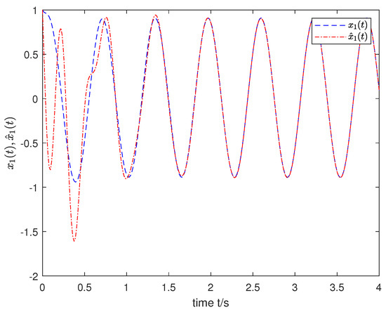
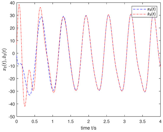
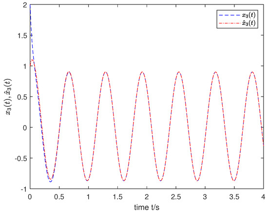
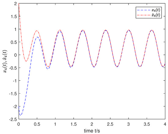
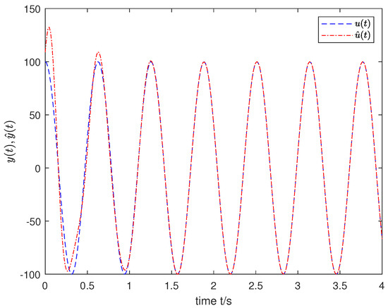
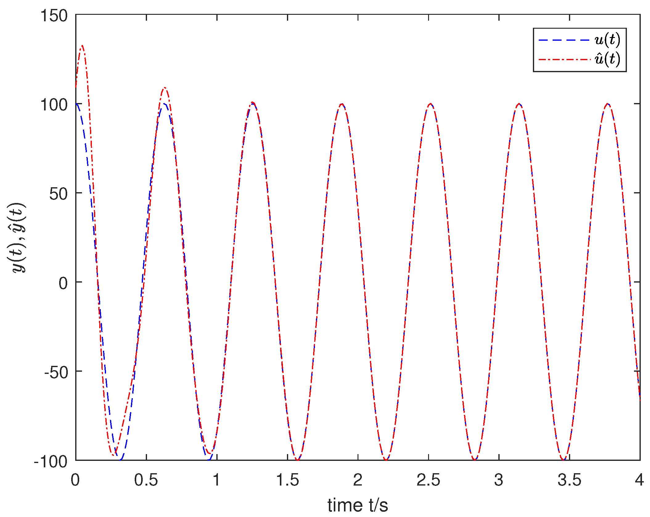
We used a MATLAB procedure (FDE12), which solves an initial value problem for a nonlinear differential equation of fractional-order (FDE). The code implemented the predictor corrector PECE method of Adama–Bashforth–Moulton type to obtain the simulation results. To properly show the effectiveness of the desired observer for the joint estimation of both states and unknown inputs, the input was selected as and the order was fixed as with the initial state . The simulation results are shown in Figure 1, Figure 2, Figure 3, Figure 4 and Figure 5, which indicate that the state and input of nonlinear FOSs can be tracked effectively by the designed observer.
Figure 1.
The estimation of state .
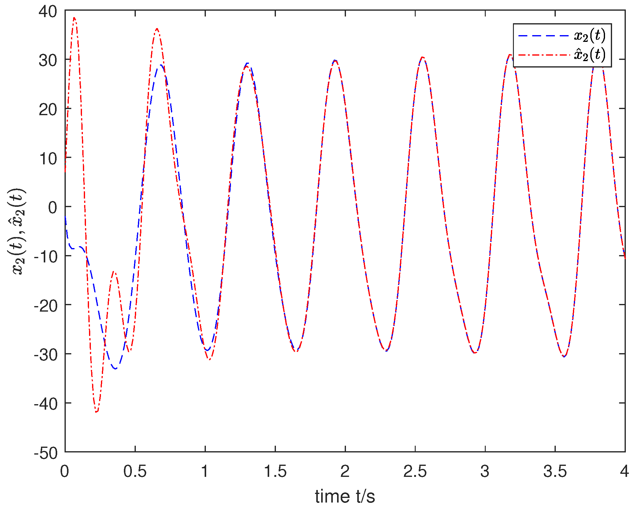
Figure 2.
The estimation of state .
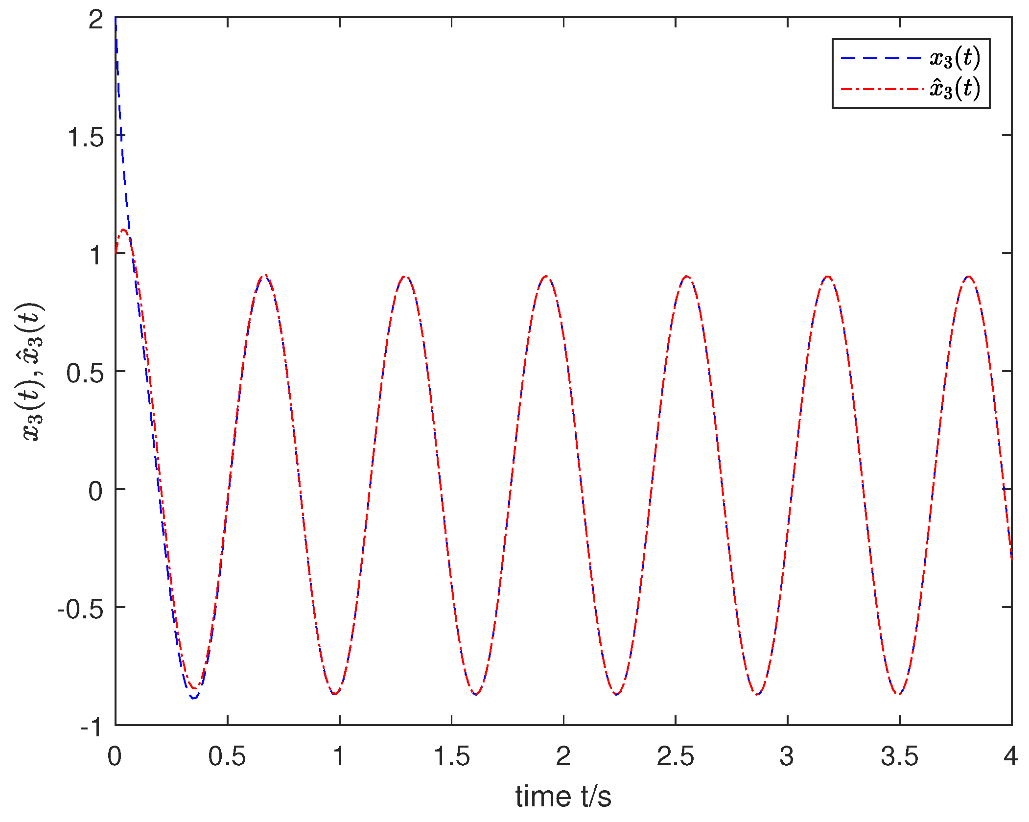
Figure 3.
The estimation of state .
Figure 4.
The estimation of state .
Figure 5.
The estimation of state .
Remark 3.
As can be seen from the simulation results, compared with [23,24,25], Algorithm 1 presented for the observer design is efficient for the joint estimation of the state and the unknown input for a class of nonlinear FOSs, where one portion satisfies the Lipschitz condition and the other does not necessarily satisfy such a condition.
| Algorithm 1 Observer Design Algorithm for the Nonlinear FOS |
|
5. Conclusions
This article designed an observer for a class of nonlinear FOSs that do not essentially satisfy the Lipschitz condition to estimate both the states and unknown inputs simultaneously. The parameterized matrices of the designed observer were derived based on the LMI technique and the property of the generalized inverse matrices combined with the Mittag–Leffler stability. The algorithm to determine the parameters of the desired observer effectively is presented. The simulation results of a numerical example are presented to verify the efficiency of the obtained algorithm.
In the future, we will study the simultaneous estimation of the state and the unknown input for variable-order nonlinear FOSs and the robustness of the designed observer.
Author Contributions
Writing—original draft preparation: C.P.; writing—review and editing: C.P. and H.Y.; methodology: C.P. and H.Y.; software: L.R.; supervision: C.P., A.Y. and L.R.; investigation: C.P. and A.Y.; formal analysis: C.P., A.Y. and L.R.; and funding acquisition: C.P. All authors have read and agreed to the published version of the manuscript.
Funding
This work was supported by National Natural Science Foundation of China under Grant 62203247.
Data Availability Statement
Data are contained within the article.
Conflicts of Interest
The authors declare no conflicts of interest.
References
- Narayanan, G.; Ali, M.S.; Alsulami, H.; Stamov, G.; Stamova, I.; Ahmad, B. Impulsive security control for fractional-order delayed multi-agent systems with uncertain parameters and switching topology under DoS attack. Inf. Sci. 2022, 618, 169–190. [Google Scholar] [CrossRef]
- Durdu, A.; Uyaroglu, Y. The shortest synchronization time with optimal fractional order value using a novel chaotic attractor based on secure communication. Chaos Solitons Fractals 2017, 104, 98–106. [Google Scholar] [CrossRef]
- Vafaei, V.; Akbarfam, A.J.; Kheiri, H. A new synchronisation method of fractional-order chaotic systems with distinct orders and dimensions and its application in secure communication. Int. J. Syst. Sci. 2021, 52, 3437–3450. [Google Scholar] [CrossRef]
- Soleimanizadeh, A.; Nekoui, M.A. Optimal type-2 fuzzy synchronization of two different fractional-order chaotic systems with variable orders with an application to secure communication. Soft Comput. 2021, 25, 6415–6426. [Google Scholar] [CrossRef]
- Shen, Y.J.; Hua, J.; Fan, W.; Liu, Y.L.; Yang, X.F.; Chen, L. Optimal design and dynamic performance analysis of a fractional-order electrical network-based vehicle mechatronic ISD suspension. Mech. Syst. Signal Process. 2023, 184, 109718. [Google Scholar] [CrossRef]
- Sarafraz, M.S.; Tavazoei, M.S. Realizability of fractional-order impedances by passive electrical networks composed of a fractional capacitor and RLC components. IEEE Trans. Circuits Syst. I Regular Papers 2015, 62, 2829–2835. [Google Scholar] [CrossRef]
- El-Saka, H.A.A.; Lee, S.; Jang, B. Dynamic analysis of fractional-order predator-prey biological economic system with Holling type II functional response. Nonlinear Dyn. 2019, 96, 407–416. [Google Scholar] [CrossRef]
- Srivastava, H.M.; Dubey, V.P.; Kumar, R.; Singh, J.; Kumar, D.; Baleanu, D. An efficient computational approach for a fractional-order biological population model with carrying capacity. Chaos Solitons Fractals 2020, 138, 109880. [Google Scholar] [CrossRef]
- Xie, Y.K.; Wang, Z.; Shen, H.; Li, Y.X. The dynamics of a delayed generalized fractional-order biological networks with predation behavior and material cycle. Nonlinear Anal. Model. Control 2020, 25, 745–765. [Google Scholar] [CrossRef]
- Marir, S.; Chadli, M.; Basin, M.V. Bounded real lemma for singular linear continuous-time fractional-order systems. Automatica 2022, 135, 109962. [Google Scholar] [CrossRef]
- Lu, J.G.; Zhu, Z.; Ma, Y.D. Robust stability and stabilization of multi-order fractional-order systems with interval uncertainties: An LMI approach. Int. J. Robust Nonlinear Control 2021, 31, 4081–4099. [Google Scholar] [CrossRef]
- Boukal, Y.; Darouach, M.; Zasadzinski, M.; Radhy, N.E. Robust H∞ observer-based control of fractional-order systems with gain parametrization. IEEE Trans. Autom. Control 2017, 62, 5710–5723. [Google Scholar] [CrossRef]
- Li, Y.; Chen, Y.Q.; Podlubny, I. Mittag–Leffler stability of fractional order nonlinear dynamic systems. Automatica 2009, 45, 1965–1969. [Google Scholar] [CrossRef]
- Zhao, Y.G.; Wang, Y.Z.; Zhang, X.F.; Li, H.T. Feedback stabilisation control design for fractional order non-linear systems in the lower triangular form. IET Control Theory Appl. 2016, 10, 1061–1068. [Google Scholar] [CrossRef]
- Chen, L.P.; Guo, W.L.; Gu, P.P.; Lopes, A.M.; Chu, Z.B.; Chen, Y.Q. Stability and stabilization of fractional-order uncertain nonlinear systems with multiorder. IEEE Trans. Circuits Syst. II Express Briefs 2023, 70, 576–580. [Google Scholar] [CrossRef]
- Peng, C.C.; Zhang, W.H. Back-stepping stabilization of fractional-order triangular system with applications to chaotic systems. Asian J. Control 2021, 23, 143–154. [Google Scholar] [CrossRef]
- Peng, C.C.; Zhang, W.H. Linear feedback synchronization and anti-synchronization of a class of fractional-order chaotic systems based on triangular structure. Eur. Phys. J. Plus 2019, 134, 292. [Google Scholar] [CrossRef]
- Belkhatir, Z.; Laleg-Kirati, T.M. High-order sliding mode observer for fractional commensurate linear systems with unknown input. Automatica 2017, 82, 209–217. [Google Scholar] [CrossRef]
- Wei, X.; Liu, D.Y.; Boutat, D. Nonasymptotic pseudo-state estimation for a class of fractional order linear systems. IEEE Trans. Autom. Control 2017, 62, 1150–1164. [Google Scholar] [CrossRef]
- Feng, T.; Wang, Y.E.; Liu, L.L.; Wu, B.W. Observer-based event-triggered control for uncertain fractional-order systems. J. Franklin Inst. 2020, 357, 9423–9441. [Google Scholar] [CrossRef]
- Pan, H.; Yu, X.H.; Guo, L. Admissible leader-following consensus of fractional-order singular multiagent system via observer-based protocol. IEEE Trans. Circuits Syst. II Express Briefs 2019, 66, 1406–1410. [Google Scholar] [CrossRef]
- Peng, C.C.; Ren, L.; Zhao, Z.H. Both sates and unknown inputs simultaneous estimation for fractional-order linear systems. Circuits Syst. Signal Process. 2024, 43, 895–915. [Google Scholar] [CrossRef]
- Kong, S.L.; Saif, M.; Liu, B. Observer design for a class of nonlinear fractional-order systems with unknown input. J. Franklin Inst. 2017, 354, 5503–5518. [Google Scholar] [CrossRef]
- Sharma, V.; Shukla, M.; Sharma, B.B. Unknown input observer design for a class of fractional order nonlinear systems. Chaos Solitons Fractals 2018, 115, 96–107. [Google Scholar] [CrossRef]
- N’Doye, I.; Salama, K.N.; Laleg-Kirati, T.M. Robust fractional-order proportional-integral observer for synchronization of chaotic fractional-order systems. IEEE/CAA J. Autom. Sin. 2019, 6, 268–277. [Google Scholar] [CrossRef]
- Lee, S.C.; Li, Y.; Chen, Y.Q.; Ahn, H.S. H∞ and sliding mode observers for linear time-invariant fractional-order dynamic systems with initial memory effect. J. Dyn. Syst. Meas. Control 2014, 136, 051022. [Google Scholar] [CrossRef]
- Khargonakar, P.P.; Petersen, I.R.; Zhou, K.M. Robust stabilization of uncertain linear systems: Quadratic and H∞ control theory. IEEE Trans. Autom. Control 1990, 35, 356–361. [Google Scholar] [CrossRef]
- Rao, C.; Mitra, S. Generalized Inverse of Matrices and Its Applications; Wiley: New York, NY, USA, 1971. [Google Scholar]


Disclaimer/Publisher’s Note: The statements, opinions and data contained in all publications are solely those of the individual author(s) and contributor(s) and not of MDPI and/or the editor(s). MDPI and/or the editor(s) disclaim responsibility for any injury to people or property resulting from any ideas, methods, instructions or products referred to in the content. |
© 2024 by the authors. Licensee MDPI, Basel, Switzerland. This article is an open access article distributed under the terms and conditions of the Creative Commons Attribution (CC BY) license (https://creativecommons.org/licenses/by/4.0/).