Article

Novel Numerical Investigation of Reaction Diffusion Equation Arising in Oil Price Modeling

by
Fehaid Salem Alshammari
Department of Mathematics and Statistics, Faculty of Science, Imam Mohammad Ibn Saud Islamic University (IMSIU), Riyadh 11564, Saudi Arabia
Mathematics 2024, 12(8), 1142; https://doi.org/10.3390/math12081142
Submission received: 15 March 2024 / Revised: 6 April 2024 / Accepted: 8 April 2024 / Published: 10 April 2024

Abstract

:
Consideration is given to a reaction–diffusion free boundary value problem with one or two turning points arising in oil price modeling. First, an exact (analytical) solution to the reduced problem (i.e., no diffusion term) was obtained for some given parameters. The space–time Chebyshev pseudospectral and superconsistent Chebyshev collocation method is proposed for both reaction diffusion (RDFBP) and reduced free boundary value problem. Error bounds on the discrete L 2 –norm and Sobolev norm ( H p ) are presented. Adaptively graded intervals were introduced and used according to the value of turning points to avoid the twin boundary layers phenomena. Excellent convergent (spectrally) and stable results for some special turning points were obtained for both reduced and RDFBP equations on an adaptively graded interval and this has been documented for the first time.

1. Introduction

Oil can be considered a major commodity in the world economy. There are many factors, such as interest rates and net demand, that may influence the behavior of oil prices. Over the last ten years, new factors have affected the behavior of oil prices. Some of these factors have a direct impact, such as the COVID-19 global lockdown that obviously reduced the demand on oil [1], which caused a historical futures price as, on 20 April 2020, the price of WTI-MAY 2020 futures contract closed at −37.68 per barrel [2]. Other factors have an indirect impact, such as the growing issue of climate change, which results in increasing antipathy towards oil among investors. In addition to these factors, the Russia–Ukraine war forced all parties to use oil prices as a weapon. These factors have increased the complexity of the oil prices’ behavior and created a dramatic change in futures prices.
Let us now pay attention to the modeling of oil prices; to do this, analyzing oil price over the last ten years is necessary. In particular, from this, one can see that oil price shows a bi-model character, which suggests a strong tendency to gather around one range of high oil prices and one range of low prices, resulting in two distinct peaks in its frequency distribution. Since no system of affine equations could not provide a finite number of non-unique fixed-point solutions, Goard and AbaOud [3] proposed such a kind of nonlinear model to model the bi-modal character of crude oil price data, which also include external stochastic driving force, representing the unpredictable effect of many neglected influences that will enable transitions to occur between the two basins of attraction as follows:
d p = A p , t d t + B p , t d Z = α β 1 p β 2 p β 3 p d t + σ p γ d Z
where p = p t is the price of oil at time t . A p , t = α β 1 p β 2 p β 3 p and B p , t = σ p γ   σ   a n d   γ   a r e   c o n s t a n t s represent the drift and diffusion term, respectively. Here, also, d Z is an increment in the Wiener process Z under a real probability measure, and where α > 0 ,   β 1 , β 2     a n d   β 3   are the stable low-fixed, unstable middle-fixed and stable high-fixed points, respectively. Regarding the model in Equation (1), there are several studies on various forms of it. For example, if we consider A p , t = μ p     and B p , t = σ p , we obtain the well-known geometric Brownian motion (GBM) model [4], which can be considered one of the earliest-used and simplest models to describe the movement of commodity prices. Later, Brennan and Schwartz [5] and Gabillon [6] assumed that the future movement of commodity prices follows the GBM and derives a closed-form solution for futures prices of oil under different assumptions. These assumptions include using constant parameters such as the interest rate, convenience yield and cost of physical oil. Other groups of authors suggest a mean reversion property for commodity prices, and this suggestion is considered to capture the effect of supply and demand in the commodity.
For A p , t = μ β 1 p and B p , t = σ p , we obtain a well-known model known as the Ornstein–Uhlenbeck model. Later, this model was used by Bjerksund and Ekern [7] to price European call options. Along the same line, Schwartz [8] proposed a mean-reverting model for oil prices, namely A p , t = μ β 1 ln p and B p , t = σ p , and derived a closed formula for futures prices. AbaOud and Goard [9] proposed two one-factor models with 3 / 4   power in the diffusion term, namely B p , t = σ p 3 4 , and empirically showed that their proposed models outperform other well-known models in capturing the behavior of oil prices.
Various extensions of one-factor models are also possible. These include two- and three-factor models. In the two-factor models, the convenience yield (see, for example, Gibson and Schwartz [10], and Schwartz [8]) and long-run mean (see, for example, Gabillon [6], Pilipovic [11] and Schwartz and Smith [12]) are the most popular choices for the second factor. In the three-factor models, some authors used interest rate as an additional factor to the spot price and convenience (see, for example, Schwartz [8]). Other authors used long-term spot price return as an additional factor to the spot price and convenience (see, for example, Cortazar and Schwartz [13]).
If we allow the possibility of a nonzero market price of risk, λ p , t , then associated oil process and risk-neutral development should be as follows:
d p = α β 1 p β 2 p β 3 p λ p , t σ p γ d t + σ p γ d Z ¯ ,
where Z ¯ is a Wiener process under an equivalent risk-neutral probability measure under which p becomes a martingale. In the book by Wilmott [14], the reaction–diffusion free boundary value problem or variable coefficient linear parabolic partial differential equation that predicts the future prices of oil under the risk-free neutral process as follows:
d p = α β 1 p β 2 p β 3 p d t + σ p γ d Z ¯ ,
can be given as follows:
F τ = σ 2 p 2 γ 2 F p p + α β 1 p β 2 p β 3 p F p ,
with
F p , 0 = p i n i t i a l   c o n d i t i o n   f o r   t i m e   v a r i a b l e ,
where no boundary conditions are imposed (its daily price determined by the stock market). To ensure that the solution is independent on any dimension, we need to nondimensionalize the equation, defining the dimensionless variable and parameters as follows:
u = F β 1 , y = p β 1   a n d   t = τ α β 1 2 .
Then, (4) can be written in the dimensionless form as follows:
u t = Γ y 2 γ 2 u y 2 + 1 y q 2 y q 3 y u y ,   w h e r e   Γ = σ 2 β 1 2 γ 4 2 α
with
u y , 0 = y .
Literature reviews reveal that there is no numerical study to find the approximate solution to Equations (6) and (7). This is mainly due to the lack of boundary condition in y direction. In this paper, both the Chebyshev pseudospectral and superconsistent Chebyshev collocation methods [15,16,17,18,19,20,21,22] are implemented in both space and time to approximate the solution to Equations (6) and (7). These methods are spectrally highly accurate methods, even for a small number of grid points. The method considered here can be regarded as a global method because the computation at any given point depends not only on the information from neighboring points but also on the information from the entire domain. In this method, the use of an orthogonal basis is more convenient and produces more accurate results. We also note that, recently, this method has been used extensively for a variety of different well-known ordinary or partial differential equations. The authors reported excellent stable and convergence results [20,21,22,23,24,25,26].
The major contributions of this paper are as follows:
  • Finding the exact (analytical) solution to the reduced problem Γ = 0   i n   E q u a t i o n   ( 7 ) for given q 2 and q 3 ;
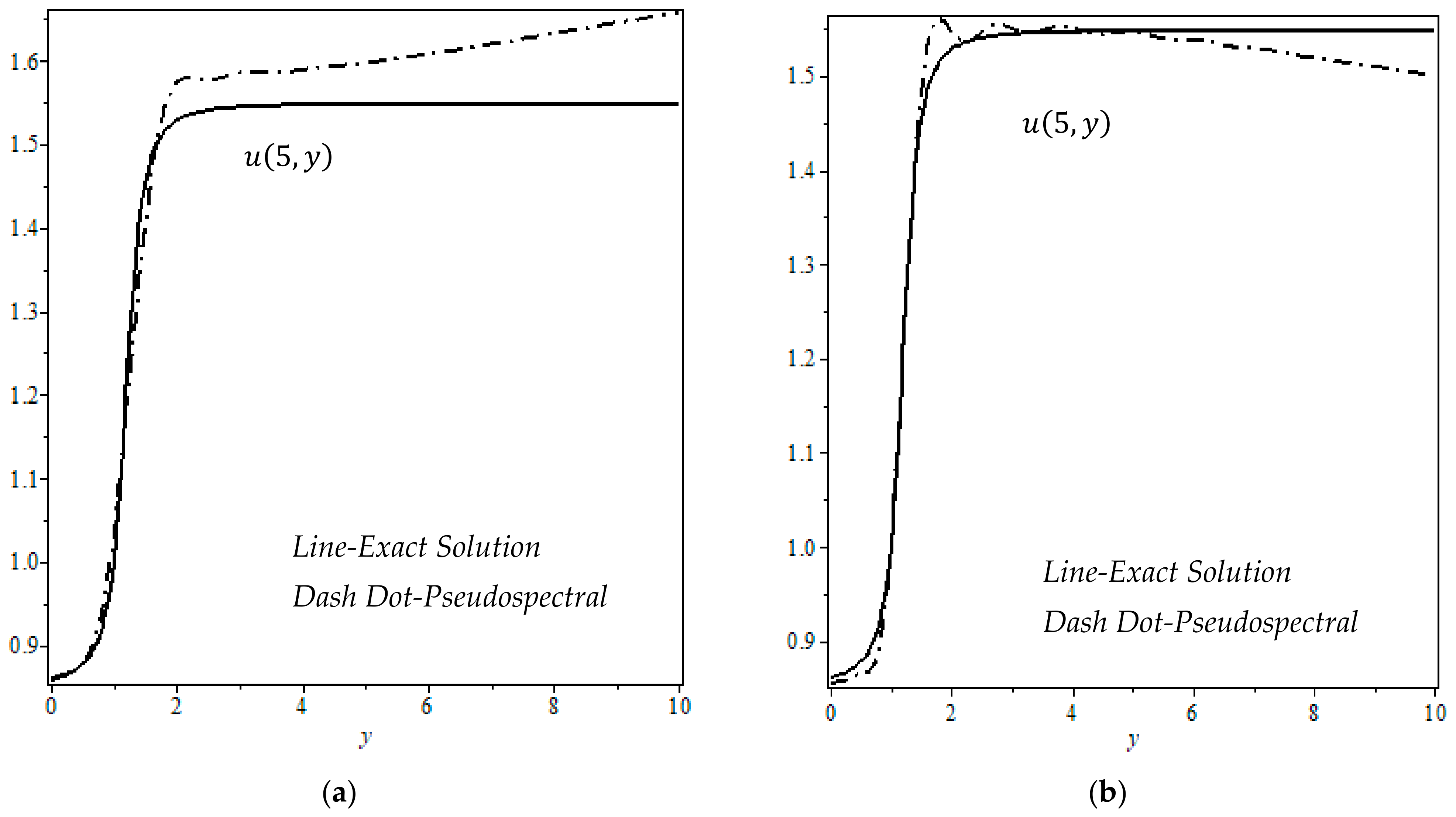
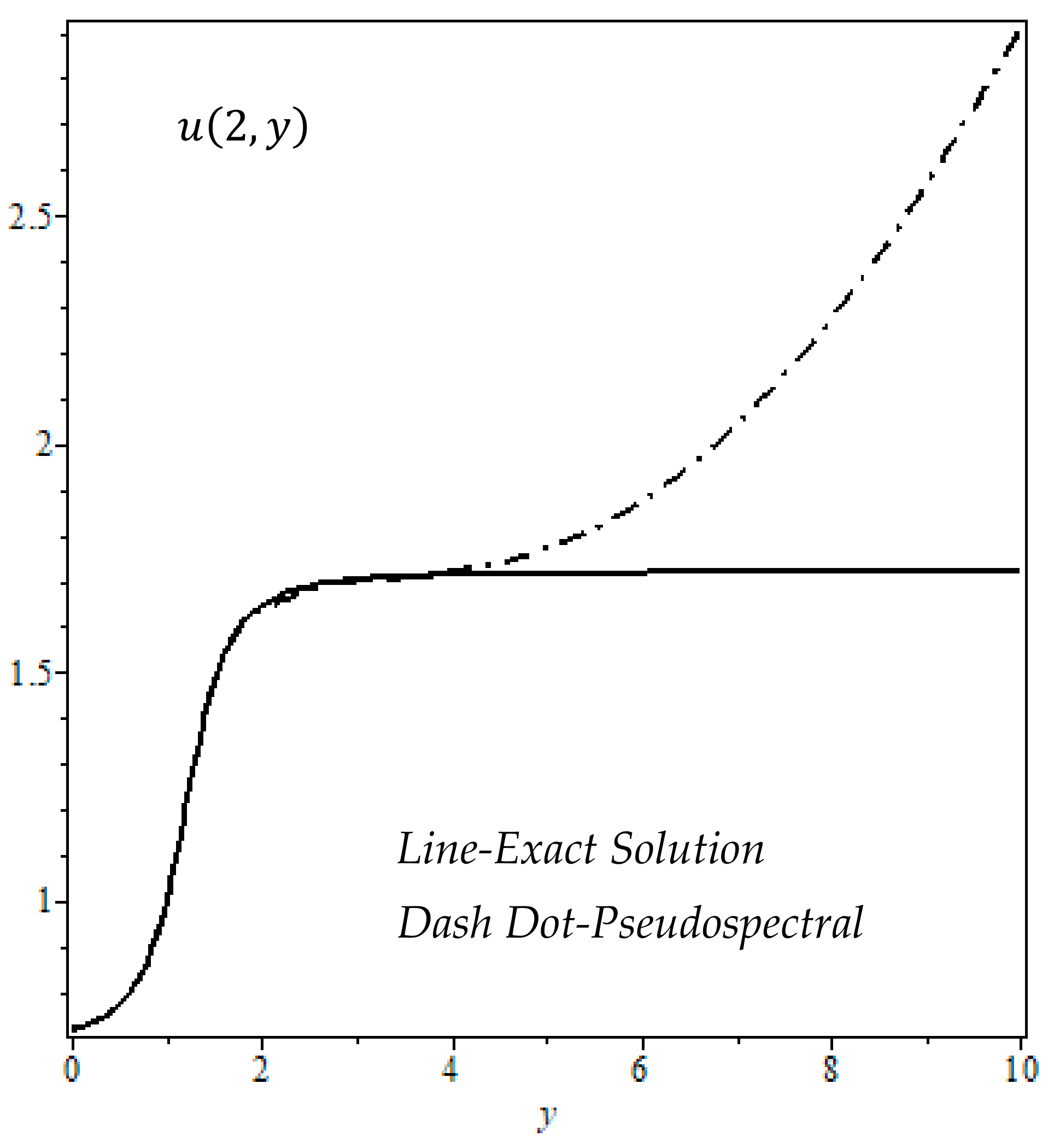
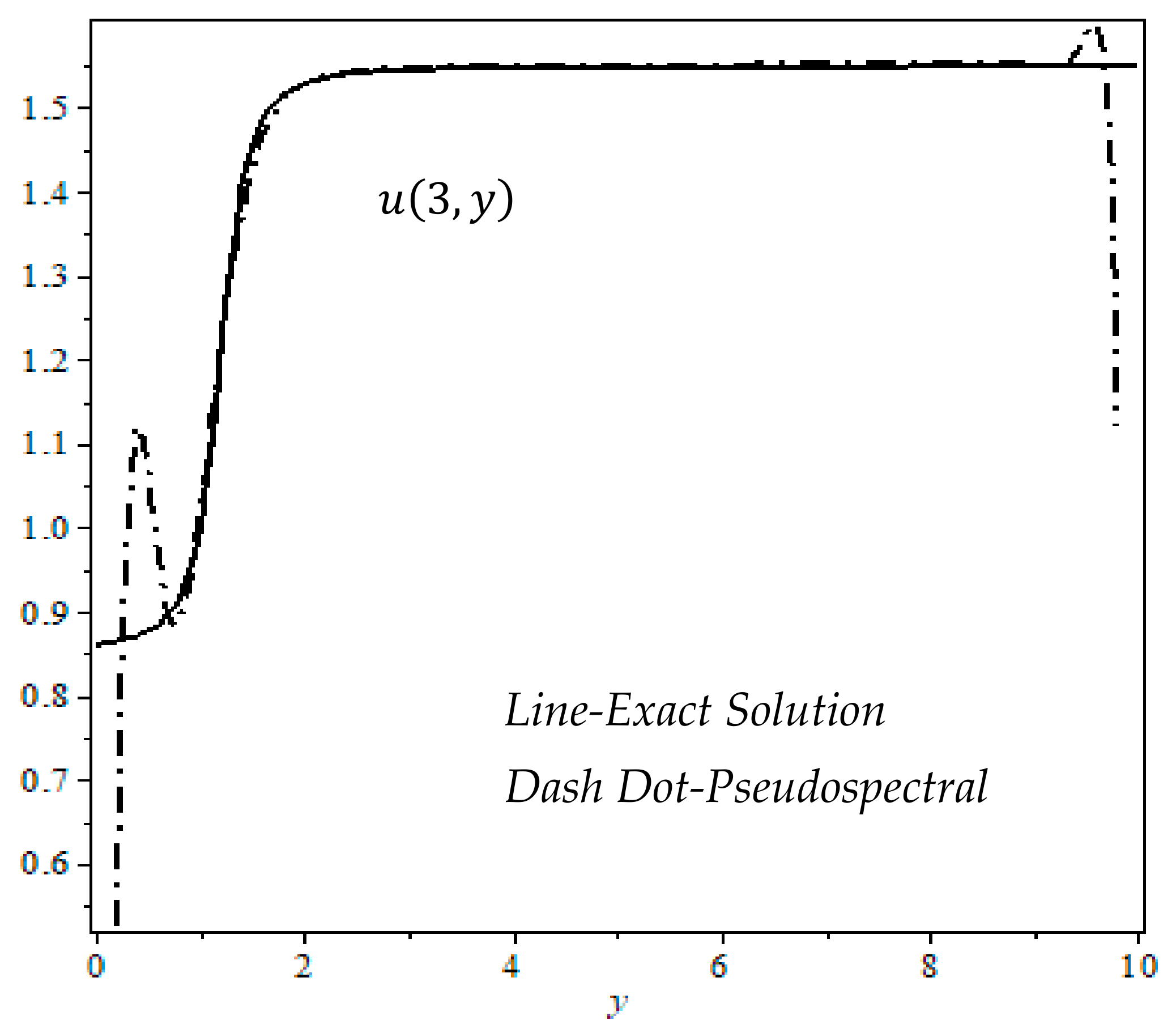
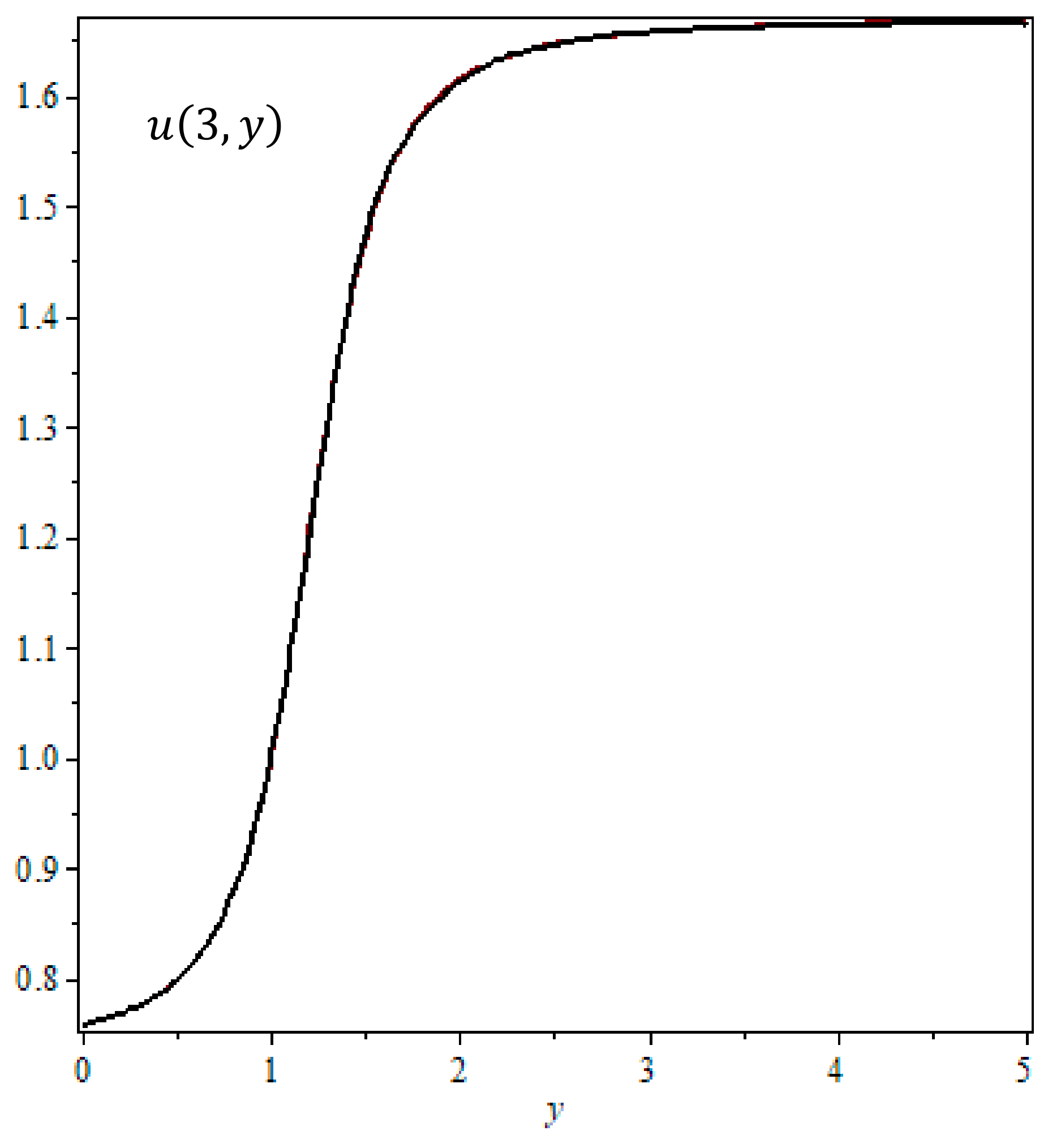
  • Constructing a scheme based on both the Chebyshev pseudospectral method and the superconsistent Chebyshev collocation method in time and space directions for the solution to the reduced problem of Equation (7) and RDFBP Equation (7) on the graded interval and compare with an analytic (exact) solution;
  • The theory of error estimate and convergence analysis for a fully discrete solution is derived for the Chebyshev pseudospectral method;
  • We also discuss the convergence rates for the pseudospectral solutions.
The importance of this paper is twofold; firstly, this is the first paper application of the space–time Chebyshev pseudospectral method to the variable coefficient reaction diffusion free boundary value problem; secondly, the authors in financial mathematics can easily use our approximation to predict the future price of crude oil.
The outline of this paper is organized as follows. In Section 2, we present the exact (analytical) solution to the reduced problem. In Section 3, we define the pseudospectral method briefly, with some important preliminaries. Error estimates for interpolating orthogonal polynomials are presented in Section 4, numerical examples are discussed in detail in Section 5, and the conclusion of our study is given in the last section.

2. Analytic Exact Solution to Reduced Problem of Equation (7)

For Γ = 0 , the equation reduces to the following:
u t = 1 y q 2 y q 3 y u y , u 0 , y = y ,
where q 2 and q 3 are positive constants such that 1 q 2 q 3 . We now have three passible cases.
1.
F o r   q 2 = q 3 = 1 , Equation (9) can be rewritten as follows:
u t = 1 y 3 u y , u 0 , y = y .
Solving (10) by the method of characteristics gives the following:
u t , y = F 2 t y 2 4 t y + 2 t + 1 2 y 1 2 ,
implementation of the initial condition, u 0 , y = y = F 1 2 y 1 2 ; so, then, we find the following:
u t , y = 1 + y 1 2 t y 2 4 t y + 2 t + 1 .  
2.
For 1 < q 2 = q 3 , Equation (7) yields the following:
u t = 1 y q 2 y 2 u y ,   u 0 , y = y .
Solving (13) by the method of characteristics achieves the following:
t , y = F t y q 2 2 + t q 2 3 + 2 t y q 2 2 t q 2 2 + ln y 1 y ln y 1 q 2 ln ( q 2 + y ) y + ln q 2 + y q 2 t y + t q 2 q 2 + 1 q 2 1 2 q 2 + y .
When we say that the analytic (exact) inverse is not possible, we mean that a closed-form solution like Equation (12) is not possible in this case. Nevertheless, we have a pseudospectral solution concerning this case, which will be given in the next section.
3.
For 1 < q 2 < q 3 , using the method of characteristic provides the following:
u t , y = F t ln y q 2 q 2 1 q 3 q 2 + ln y q 3 q 3 1 q 3 q 2 + ln y 1 q 2 1 q 3 1 = I y q 3 1 q 3 1 q 3 q 2 y 1 1 q 2 1 q 3 1 e t y q 2 1 q 2 1 q 3 q 2 .
Hence, the application of the initial condition yields the following:
u 0 , y = y = I y q 3 1 q 3 1 q 3 q 2 y 1 1 q 2 1 q 3 1 y q 2 1 q 2 1 q 3 q 2 .
If we let
y q 3 1 q 3 1 q 3 q 2 y 1 1 q 2 1 q 3 1 y q 2 1 q 2 1 q 3 q 2 = Σ ,
then
y q 3 q 2 1 y 1 q 3 q 2 y q 2 q 1 1 = Σ q 3 1 q 3 q 2 q 2 1 .
For a given rational value of q 2 and q 3 , we can solve the value of y , so we can identify the function in (15), and the solution to Equation (7) can be obtained.
4.
For y = 1 or y = q 2 or y = q 3 , in this case, for example y = 1 ;
u t t , 1 = 0 ,   h e n c e   u t , 1 = C ,
But, from the initial condition, we have u t , 1 = 1 ; based on the same discussion, we can find u t , q 2 = q 2 and u t , q 3 = q 3 .
It is not possible to obtain the exact analytic solution to Equation (7); there are several methods to find the approximate solution. In [3], the authors applied a regular perturbation method to obtain the approximate analytic solution to the problem, where the perturbation parameter ε appears in Equation (7). Since perturbation methods rely on there being a dimensionless parameter in a problem that is relatively small: ε≪1, the solution has a limited range of validity. Therefore, we propose here a pseudospectral method to obtain the approximate analytical solution. We note here that there is no limited range of validity for the method that we have suggested in this paper.

3. Time–Space Chebyshev Pseudospectral Method

We assume that the solution to the problem in (7) can be expressed by the finite linear combination of the product of Chebyshev polynomials in both dimensionless time and price space, i.e., the following:
I M u t , x = i = 1 M j = 0 M C i j T i t T j x ,
where T i ζ and T j y are the Chebyshev polynomials in time and price directions and C i j the discrete expansion coefficient, and can be calculated easily as follows:
C i j = 1 η i η j p = 0 M q = 0 M T i t p T j x q ω ζ p ω y q u ζ p , x q ,
where η i , η j are the discrete normalization constants and ω is the weight function. By substituting (21) into (20) and arrange the terms using the properties of Chebyshev polynomials [21], we obtain the following:
I M u t , x = i = 1 M j = 0 M է i M t է i M x u t i , x j ,
here, է i are the Lagrange polynomials (using Christoffel-Darboux identity [16,22]) defined by the following:
է l z = ω l i = 1 j = 0 M 1 η i T i z i T i z i = 1 l + 1 1 z 2 c l M 2 z z l z T M z ,
where above z is generic variable as z = t , y and
c l = 2 , l = 0   and   M , 1 ,   0 < l < M .
This formula, based on Chebyshev–Gauss points, was also used in this study. But, in this scheme, the inverse mentioned above is not valid (21) and (22), so we apply the collocation method directly; even if the determinant of the resulting matrix is very big, we are able obtain convergent results easily and comparable them with the Chebyshev pseudospectral method.
If we set the following:
Ξ 1 M t = է 1 t , , է M t T   a n d   Ξ 0 M x = է 0 t , , է M t T .
then we express (22) in a vector–matrix form by using the Kronecker product as follows:
I M u t , y = Ξ 1 M t Ξ 0 M x T U ,
where U is the M M + 1 -vector:
U = U 10 , , U 1 M U 20 , , U 2 M | U M 0 , , U M M T
since
d d t Ξ 1 M T t = Ξ 1 M T t D 2 : M + 1,2 : M + 1 ( 1 ) .
This is actually derived from the expansion of derivatives [20,27], where D M ( 1 ) is called the differential or derivative matrix, with M being its dimension and given by [20,21,27] the following:
D i j 1 = P z i Q z j z i z j ,   i j ,   l = 0 , l i r z i z j 1 , i = j .  
Therefore,
t I M u t , x = t Ξ 1 M T t Ξ 0 M T x U = Ξ 1 M T t D 2 : M + 1,2 : M + 1 1 Ξ 0 M T x U = Ξ 1 M t Ξ 0 M x T D 2 : M + 1,2 : M + 1 1 I M + 1 U ,
where I M + 1 is the M + 1 X   M + 1   identity matrix.
Similarly, we find the following:
x I M u t , x = Ξ 1 M t Ξ 0 M x T I M D 1 : M + 1 , 1 : M + 1 1 U .
We can now transform the space 0 , A and time 0 , T to 1 , 1
t = 1 2 T + 1 2 T t * ,   y = 1 2 A + 1 2 A x .  
Using this transformation in Equations (7) and (8), we obtain the following:
2 T u t * 2 A 1 G x q 2 G x q 3 G x u x 4 A 2 Γ G x 2 γ 2 u x 2 = 0 ,  
where G x = 1 2 A + 1 2 A x   and the initial condition; also, we omit the star expression in the dimensionless t direction as follows:
u 0 , x = 1 2 A + 1 2 A x .  
We now use Equations (25)–(30) to substitute into (32); as a result, we obtain the following:
2 T Ξ 1 M t Ξ 0 M x T D 2 : M + 1,2 : M + 1 1 I M + 1 U 2 A 1 G x q 2 G x q 3 G x Ξ 1 M t Ξ 0 M x T I M D 1 : M + 1 , 1 : M + 1 1 U 4 A 2 ε G x 2 γ Ξ 1 M t Ξ 0 M x T I M D 1 : M + 1 , 1 : M + 1 2 U = 0
and the initial condition
Ξ 1 M 1 Ξ 0 M x T V = 1 2 A + 1 2 A x ,  
where V = V 00 , , V 0 M T . Now, using the Chebyshev–Gauss collocation points, we obtain a system of linear equation, the important points at this stage, and the best collocation points, such that the solution to the equation is stable and consistent. We solved this major problem, which can be seen in the numerical solution section.

4. Error Analysis

In this section, we will find the error bound for the numerical solution. To do this, we need the following definitions.
Definition 1.
Let  Ω  and open subset of   R  and if  ω 0  is a weight function that is a locally integrable function, we write  f L q Ω ¯ ,   ω ,   1 q < , if  f :   Ω ¯ = a , b C  is measurable on  Ω ¯  and the norm is defined by the following:
f L q Ω ¯ ,   ω = a b f t p ω t d t 1 q < .  
For  p N , the Sobolev space  W ω p , q Ω ¯  is defined by the following:
W ω p , q Ω ¯ = f L q Ω ¯ ,   ω : α f L q Ω ¯ ,   ω   α p   ,  
where the derivatives are in the distribution sense. When this space is endowed with the norm
f W ω p , q Ω ¯ = α p α f W ω p , q Ω ¯ .
W ω p , q Ω ¯  is a Banach space. For  q = 2 , this space is denoted by  H w p Ω ¯ .
Theorem 1.
Let  u t , x H ω p 1 , 1 , then there exists a constant  C , such that the following inequality holds:
u t , x I M u t , x L ω 2 1 , 1 C M p u t , x H ω p 1 , 1
Proof. 
Since we are looking for the approximate solution obtained from Chebyshev expansion, that is the following:
P M u t , x = u M t , x = j = 0 M i = 1 M a i j T i t T j x ,
where the coefficient follows from the orthogonality of Chebyshev polynomials as follows:
a i j = 1 η i η j 1 1 1 1 u M t , x T i t T j x ω i t ω j x d x d t .
Now, using the Chebyshev differential equation, we find Chebyshev operators [20]:
n 2 F z ω z = z 1 z 2 1 / 2 z F z = Δ l F z ω z , l = 1,2 .
where, above Δ 1 and Δ 2 , are the Chebyshev operators in direction time and space such that Δ 1 Δ 2 = Δ and n = 0,1 , 2 , …. Since Chebyshev polynomials satisfy this property, we can rewrite (40) in terms of (41) as follows:
a i j = 1 η i η j 1 1 T i t ω i t R j t   d t ,   R j t = 1 1 u M t , x j 2 x 1 x 2 1 / 2 x T j x d x .  
Take the following:
R j t = 1 1 u M t , x j 2   x 1 x 2 1 / 2 x T j x d x .  
By integrating the parts above, we find the following:
R j t = 1 j 2 [ u M t , x 1 x 2 1 / 2 x T j x | x = 1 x = 1 + 1 1 x u M t , x 1 x 2 1 / 2 x T j x d x ] = 1 j 2 1 1 x u M t , x 1 x 2 1 / 2 x T j x d x .
By integrating the parts again and using (41), we find the following:
R j t = 1 j 2 x u M t , x 1 x 2 1 / 2 T j x | x = 1 x = 1 1 j 2 1 1 T j x x 1 x 2 1 2 x u M t , x d x = 1 j 2 1 1 T j x x 1 x 2 1 2 x u M t , x d x = 1 j 2 1 1 1 u M t , x T j x ω x d x .  
By substituting into 43 , we achieve the following:
a i j = 1 η i η j j 2 1 1 1 1 1 u M t , x T i t T j x ω t ω x d x d t .
We can do same in time direction and obtain the following:
a i j = 1 η i η j i 2 j 2 1 1 1 1 1 2 u M t , x T i t T j x ω t ω x d x d t = 1 η i η j i 2 j 2 1 1 1 1 Δ u M t , x T i t T j x ω t ω x d x d t .
This can be repeated m t i m e s , which provides the following:
a i j = 1 η i η j i j 4 m 1 1 1 1 Δ m u M t , x T i t T j x ω t ω x d x d t .
From Cauchy–Schwarz, we obtain the following:
a i j 2 C i j 4 m Δ m u M x , t L ω 2 1 , 1 2 ,  
since Δ u m x , t L ω 2 2 u m x , t H ω 4 2 by definition, then we obtain, from the above, the following:
a i j 2 C i j 4 m u M x , t H ω 4 m 1 , 1 2
This inequality can be extended to an infinite number of sums, in which case, the inequality becomes as follows:
a i j 2 C i j 4 m u x , t H ω 4 m 1 , 1 2 .
The difference between the Chebyshev spectral solution and Chebyshev pseudospectral solution is called the aliasing error:
R M u = I M u P M u .
It is not difficult to see that the aliasing error is only affected by the truncation error. Applying the Pythagoras theorem, we obtain the following:
u I M u L ω 2 1 , 1 2 u P M u L ω 2 1 , 1 2 + R M u L ω 2 1 , 1 2 ,
where R M u is defined as follows:
R M u = i = 1 M j = 0 M 1 η i η j l > M k > M T i t , T l t ω T j x , T k x ω a i j T i t T j x ,  
where
T j z , T k z ω = l = 0 M T j z l , T k z l ω k = 1 1 T j z . T k z ω z d z =   0 ,   j k ,   π ,   i = 0 , M   a n d   j = k ,   π 2 ,   i = 1,2 , . . .   M 1   a n d   j = k .    
Hence, it is clear that R M u = 0 because T i t , T l t are orthogonal with respect to the weight function and i j (because of the range of summation). Therefore, we obtain the following:
u I M u L ω 2 1 , 1 2 = u P M u L ω 2 1 , 1 2 ,  
since
u P M u = i = M + 1 j = M + 1 a i j T i t T j x ,  
or
u P M u L ω 2 1 , 1 2 = i = M + 1 j = M + 1 a i j T i t T j x L ω 2 1 , 1 2 = i = M + 1 j = M + 1 η i η j a i j 2 i = M + 1 j = M + 1 η i η j C i j 4 m u m x , t H ω 4 m 2   C u m x , t H ω 4 m 2 i = M + 1 j = M + 1 η i η j 1 i j 4 m C M 8 m u x , t H ω 4 m 2 .  
Therefore, we achieve the following:
u P M u L ω 2 1 , 1 C M 4 m u x , t H ω 4 m 1 , 1
If we rename p = 4 m above, the inequality becomes as follows:
u P M u L ω 2 1 , 1 C M p u x , t H ω p 1 , 1
Finally, by using Equation (53), we obtain the truncation terror bound for our collocation method as follows:
u I M u L ω 2 1 , 1 C M p u x , t H ω p 1 , 1
Hence, the theorem is proved. □
Similarly, we can prove that
s u z s s z s I M u L ω 2 1 , 1 C M p s u z s H ω p 1 , 1 = C M p u x , t H ω p + s 1 , 1 ,   z = t , x .  
Let us now find the truncation error for our Equation (32):
R t , x = 2 T t * u I M u 2 A 1 G x q 2 G x q 3 G x x u I M u 4 A 2 ε G x 2 γ 2 x 2 u I M u 2 8 T 2 t * u I M u 2 + 16 A 2 1 G x q 2 G x q 3 G x 2 x u I M u 2 + 4 4 A 2 ε G x 2 γ 2 2 x 2 u I M u 2 .
Through the double integration of both sides with respect to t * and x on 1 , 1 x 1 , 1 , and using the Minkowski inequality, we obtain the following:
E ¯ C δ 1 M p u x , t H ω p + 1 1 , 1 + δ 2 M p u x , t H ω p + 2 1 , 1 .

5. Numerical Results and Discussion

First, we solve the reduced problem (9), where analytical solution is possible, then we demonstrate how the numerical solution develop and converge the exact solution, to do this we select q 2 = 1 + ε and q 3 = 1 + 2 ε , in this case analytical (exact) solution is given by
u t , y = 1 + ε 1 + y q 2 q 2 y 2 e 2 ε 2 t 1 y q 3 y
In Figure 1, Figure 2 and Figure 3, we compared the exact solution with the semi-analytical solution obtained from the space–time pseudospectral Chebyshev method for ε = 0.2 , t , y ϵ 0,10 × 0,10 . We focused on the effect of turning points; in this case, y = 1,1.2   a n d   1.4 are the turning points and u t , 1 = 1 ,   u t , 1.2 = 1.2 and u t , 1.4 = 1.4 are the solutions. In Figure 1a, we used 24 × 24 Chebyshev points; we saw that the numerical solution increases with an increase in the value of y , but the exact solution reaches its maximum around y = 2 . Beyond this point, solutions show steady behavior. When we increased the number of points to 28 × 28, the numerical solution again deviated from the exact solution in the initial phase and after y > 2 , as documented in Figure 1b. In Figure 2, we checked the numerical solution at t = 2 , and saw that the difference between the exact and approximate solutions is less than 10 2 for y < 4 . This suggests the use of the adaptively graded interval. The other interesting point in the present problem is the boundary layer formation. In Figure 3, we showed the twin boundary layer where we used equally distributed collocation points in both dimensionless time and space directions. We then considered the graded interval t , y ϵ 0,5 × 0,5 ,   0,10 × 0,5 and 0,10 × 0,5 , then we covered t , y ϵ 0,10 × 0,10 again. Figure 4 shows both the exact solution and approximate analytical solution on graded interval at t = 3 ; we see excellent convergence of our numerical method to the exact solution. Indeed, we see from Figure 5 that the error, which is the difference of approximate solution to exact solution, is bounded by e 3.5 × 10 5 . But when we increase the value of t , the error also increases. Next, we solved the full problem, in which case the exact solution was not possible. Figure 6a,b show the effect of the second-order derivative on the future price of oil for fixed Γ = 0.05 and Γ = 0.25 , r e s p e c t i v e l y . Figure 6a represents the development of the future price of oil with dimensionless price direction for t = 0.625 ; we see that increasing the value of Γ would cause an initial increase in the value of the future price of oil, but it would eventually reduce the future price of oil. We observed similar behavior at dimensionless time t = 4.35 , as shown in Figure 6b, where q 2 = 1.2 and q 3 = 1.4 , and we achieved the exact solution for Γ = 0 (Equation (65)). In this case, we also checked the development of the future of oil prices with dimensionless time variable for fixed y = 0.625 and y = 4.35 in Figure 7a,b, respectively. As we expected, increasing the value of Γ would cause an increase in the value of the future price of oil initially (Figure 7a) but, later in time, it would decrease the value of the future price of oil (Figure 7b). Let us see how the solution turns out with the value of y . If y < 1 , the future price of oil increases with the value of the space variable; if y > 1 , the future price of oil decreases while the space variable increases. This can also be seen in Figure 7a,b; we also observed, depending on the value of the turning points, that the solution can turn three times. This is why we need more and more collocation points to obtain enough accuracy, but more collocation points make the matrix ill-conditioned. Hence, in this study, we balanced these two factors.
Next, we solved the full problem, in which case the exact solution was not possible. For this example, we selected parameters q 2 = 1.75   a n d   q 3 = 2 . Figure 8a–c show the effect of the second-order derivative on the future price of oil for a fixed value of the dimensionless time variable as t = 2 ,   0.5   a n d   3.5 . We find exactly the same behavior as before; the value of Γ initially increases, which means an increase in the price of oil, but later reverses, and the price of oil decreases. In Figure 9a–c, we fix the value–space variable as y = 0.2 ,   2   a n d   3.5 and the development of the future price of oil with dimensionless time. We see, again, an increase in the value of Γ and a decrease in the value of the oil price. Overall, we only selected a few turning points here; however, for every given turning point, we can select a graded interval for which our method converges and becomes stable. Specifically, we selected here γ = 1 / 2 , but when we increase this value at a certain stage, it will be very difficult to find the graded interval.
Let us check the paper of Funaro [17], where he considered the superconsisted Chebyshev collocation method. First, he suggested that we start with zeros of χ n = 1 x 2 T n x , then define the operator L = ε 2 x 2 + β x so that
ε χ n z i + β χ n z i = 0 , i = 1,2 , . . . n 1 .
We considered some simplified cases of our problem and applied the collocation points obtained from Equation (6); we did not find any significant difference between the Chebyshev pseudospectral solution with Chebyshev collocation points and the superconsisted Chebyshev pseudospectral method with collocation points from (66).

6. Conclusions

In this study, consideration was given to the reaction–diffusion free boundary value problem (singularly perturbed RDFBP) and we showed the following:
  • For the Γ = 0 (i.e., first-order hyperbolic equation or reduced equation) case, we obtained the exact (analytical) solution for a variety of parameters involved in modeling;
  • We used the pseudospectral Chebyshev collocation method to obtain the approximate analytical solution to the reduced problem on the graded interval and spectral convergence of the method observed for the solution;
  • We used the above method for the approximate analytical solution to the RDFBP problem (for the existence of the solution, see, for example, Freidman [28] or E. Süli et al. [29]) and the effect of the second-order term on the future price of oil, discussed in detail.
As far as the literature is concerned, these problems have never been solved before. In future studies, we will consider the RBFBF with mixed-boundary condition problems.

Funding

The authors extend their appreciation to the Deputyship for Research & Innovation, Ministry of Education in Saudi Arabia for funding this research through the project number IFP-IMSIU-2023095. The authors also appreciate the Deanship of Scientific Research at Imam Mohammad Ibn Saud Islamic University (IMSIU) for supporting and supervising this project.

Data Availability Statement

The author confirms that the data supporting the findings of this study are available within the article.

Conflicts of Interest

The author declares no conflicts of interest.

References

  1. Wang, Q.; Li, S.; Zhang, M.; Li, R. Impact of COVID-19 pandemic on oil consumption in the United States: A new estimation approach. Energy 2022, 239, 122280. [Google Scholar] [CrossRef] [PubMed]
  2. Limakrisna, N.; Setiawan, E.B.; Agusinta, L.; Firdianyah, R.; Ricardianto, P.; Indupurnahayu, I.; Suryawan, R.F.; Sari, M.; Mulyono, S.; Sakti, R.F.J. Changes in demand and supply of the crude oil market during the COVID-19 pandemic and its effects on the natural gas market. Int. J. Energy Econ. Policy. 2021, 11, 1–6. [Google Scholar] [CrossRef]
  3. Goard, J.; AbaOud, M.A. Bimodal Model for Oil Prices. Mathematics 2023, 11, 2222. [Google Scholar] [CrossRef]
  4. Ross, S.M. Introduction to Probability Models; Academic Press: Cambridge, MA, USA, 2014. [Google Scholar]
  5. Brennan, M.; Schwartz, E. Evaluating Natural Resource Investments. J. Bus. 1985, 58, 135–157. [Google Scholar] [CrossRef]
  6. Gabillon, J. The Term Structures of Oil Futures Prices; Oxford Institute for Energy Studies: Oxford, UK, 1991. [Google Scholar]
  7. Bjerksund, P.; Ekern, S. Contingent claims evaluation of mean-reverting cash flows in shipping. In Real Options in Capital Investment: Models, Strategies, and Applications; Greenwood Publishing Group: Westport, CT, USA, 1995; pp. 207–219. [Google Scholar]
  8. Schwartz, E. The stochastic behaviour of commodity prices: Implications for valuation and hedging. J. Financ. 1997, 3, 923–973. [Google Scholar] [CrossRef]
  9. AbaOud, M.; Goard, J. Stochastic Models for Oil Prices and the Pricing of Futures on Oil. Appl. Math. Financ. 2015, 22, 189–206. [Google Scholar] [CrossRef]
  10. Gibson, R.; Schwartz, E. Stochastic Conveience Yield And The Pricing of Oil Continget Claims. J. Financ. 1999, 3, 959–976. [Google Scholar]
  11. Pilipovic, D. Energy Risk: Valuing and Managing Energy Derivatives; McGraw Hill: New York, NY, USA, 1997. [Google Scholar]
  12. Schwartz, E.; Smith, J. Short-Term Variation And Long-Trem Dyanamics in Commodity Prices. Manag. Sci. 2000, 46, 893–911. [Google Scholar] [CrossRef]
  13. Cortazar, G.; Schwartz, E. Implementing a Stochastic Model For Oil Futures Prices. Energy Econ. 2003, 25, 215–238. [Google Scholar] [CrossRef]
  14. Wilmott, P. Derivatives: The Theory and Practice of Financial Engineering; John Wiley & Sons: Chichester, UK, 1998. [Google Scholar]
  15. Funaro, D. A new scheme for the approximation of advection-diffusion equations by collocation. SIAM J. Numer. Anal. 1993, 30, 1664–1676. [Google Scholar] [CrossRef]
  16. Funaro, D. Some remarks about the collocation method on a modified Legendre grid. Comput. Math. Appl. 1997, 33, 95–103. [Google Scholar] [CrossRef]
  17. Funaro, D. A superconsistent Chebyshev collocation method for second-order differential operators. Numer. Algorithms 2001, 28, 151–157. [Google Scholar] [CrossRef]
  18. Pinelli, A.; Couzy, W.; Deville, M.O.; Benocci, C. An efficient iterative solution method for the Chebyshev collocation of advection-dominated transport problems. SIAM J. Sci. Comput. 1996, 17, 647–657. [Google Scholar] [CrossRef]
  19. De l’Isle, F.; Owens, R.G. A superconsistent collocation method for high Reynolds number flows. Comput. Fluids 2023, 259, 105897. [Google Scholar] [CrossRef]
  20. Mittal, A.K. A space-time pseudospectral method for solving multi-dimensional quasi-linear parabolic partial differential (Burgers’) equations. Appl. Numer. Math. 2024, 195, 39–53. [Google Scholar] [CrossRef]
  21. Canuto, C.; Hussaini, M.Y.; Quarteroni, A.; Zang, T.A. Spectral Methods: Fundamentals in Single Domains; Springer Science & Business Media: Berlin, Germany, 2007. [Google Scholar]
  22. Canuto, C.; Hussaini, M.Y.; Quarteroni, A.; Zang, T.A. Spectral Methods: Evolution to Complex Geometries and Applications to Fluid Dynamics; Springer Science & Business Media: Berlin, Germany, 2007. [Google Scholar]
  23. Fornberg, B. A Practical Guide to Pseudospectral Methods; Cambridge University Press: Cambridge, UK, 1998. [Google Scholar]
  24. Mittal, A.K. Two-dimensional Jacobi pseudospectral quadrature solutions of two-dimensional fractional Volterra integral equations. Calcolo 2023, 60, 50. [Google Scholar] [CrossRef]
  25. Balyan, L.K.; Mittal, A.K.; Kumar, M.; Choube, M. Stability analysis and highly accurate numerical approximation of Fisher’s equations using pseudospectral method. Math. Comput. Simul. 2020, 177, 86–104. [Google Scholar] [CrossRef]
  26. Mittal, A.K.; Balyan, L.K. A highly accurate time–space pseudospectral approximation and stability analysis of two dimensional brusselator model for chemical systems. Int. J. Appl. Comput. Math. 2019, 5, 140. [Google Scholar] [CrossRef]
  27. Boyd, J.P. Chebyshev and Fourier Spectral Methods; Courier Corporation: Chelmsford, MA, USA, 2001. [Google Scholar]
  28. Friedman, A. Partial Differential Equations of Parabolic Type; Courier Dover Publications: Mineola, NY, USA, 2008. [Google Scholar]
  29. Baker, M.D.; Süli, E.; Ware, A.F. Stability and convergence of the spectral Lagrange-Galerkin method for mixed periodic/non-periodic convection-dominated diffusion problems. IMA J. Numer. Anal. 1999, 19, 637–663. [Google Scholar] [CrossRef]
Figure 1. (a,b) Comparison of pseudospectral solution with exact solution at t = 5 for q 2 = 1.2   a n d     q 3 = 1.4 in (a) 24 collocation points and in (b) 28 collocation points.
Mathematics 12 01142 g001
Figure 2. Comparison of pseudospectral solution with exact solution at t = 2 for q 2 = 1.2   a n d   q 3 = 1 . 4 and 32 collocation points.
Mathematics 12 01142 g002
Figure 3. Demonstration of twin boundary layer formation in pseudospectral solution.
Mathematics 12 01142 g003
Figure 4. Approximate analytical solution on graded interval at t = 3 for q 2 = 1.3   a n d   q 3 = 1.4 .
Mathematics 12 01142 g004
Figure 5. Difference between approximate and exact solution at t = 3 .
Mathematics 12 01142 g005
Figure 6. The effect of Γ on the future price of oil for a   t = 0.625     b   t = 4.35 .
Mathematics 12 01142 g006
Figure 7. The effect of Γ on the future price of oil for a   y = 0.625     b   y = 4.35 .
Mathematics 12 01142 g007
Figure 8. The effect of Γ on the future price of oil at (a). a   t = 2   b   t = 0.5   c   t = 3.3 for q 2 = 1.75     a n d   q 3 = 2 .
Mathematics 12 01142 g008
Figure 9. The effect of Γ on the future price of oil at (a). a   y = 2   b   y = 0.5   c   y = 3.3 for q 2 = 1.75     a n d   q 3 = 2 .
Mathematics 12 01142 g009
Disclaimer/Publisher’s Note: The statements, opinions and data contained in all publications are solely those of the individual author(s) and contributor(s) and not of MDPI and/or the editor(s). MDPI and/or the editor(s) disclaim responsibility for any injury to people or property resulting from any ideas, methods, instructions or products referred to in the content.

