Fuzzy-Based Road Accident Risk Assessment

Abstract

It is necessary to extensively investigate the causes of road accidents with the utmost precision to harness future technological advancements, such as autonomous driving and intelligent accident prevention systems. Nevertheless, since most accidents are attributed to simple human errors, unraveling the complex root-cause factors poses a considerable challenge. This is where fuzzy logic can offer a potential solution: it is essential to understand even seemingly straightforward errors, such as speeding, to identify external factors that could play a pivotal role in future accident prevention. A more in-depth examination and comprehension of elements like road curvature, slope, and their correlation with accidents are necessary. Additionally, it is crucial to explore how the frequency of accidents on specific road segments varies under diverse weather conditions. This article analyzes which curves can be considered more dangerous and the factors that render them risky. The fuzzy model presented in this article is primarily capable of estimating the risk of a given road segment based on its curvature characteristics. The model results presented in the article indicate that sections of the road can become more risky due to multiple curves and curves with a radius of less than 80 m. The model assesses risk based on the physical characteristics of road segments, primarily the curvature radius, while, typically, other road risk assessment models rely on traffic volume and accident counts.

1. Introduction

For most accidents, human inattention or irresponsibility is the triggering cause. However, it is also worthwhile to understand other reasons because if these factors can be eliminated, the number of accidents can be reduced in the future. In the case of accidents, the police or investigators determine the possible cause and issue an accident report to ascertain the exact cause and potentially identify the at-fault driver. However, it is too abstract to draw long-term conclusions about improving the road section in many cases. For example, in the case of an accident on a curve where speeding was the primary cause, the report will state that the driver could not take the curve due to speeding, but it will not include details about the properties of the curve, such as the radius and slope. Additionally, there can be abstract correlations on a given road section, such as a car easily traversing the section with even more careless driving, while, with another vehicle, such as a motorcycle, an accident can occur with minor inattention on the same road section. In David D. Clarke et al.’s [1] research, it was determined that a lack of experience among motorcyclists can lead to more significant accidents even in a simple curve situation, especially when the motorcycle belongs to the supersport category.

It can be concluded that many factors are highly abstract during investigations and can be interpreted in multiple ways, making it worthwhile to use fuzzy logic to draw conclusions. The advantage of fuzzy logic is that one of its typical applications is risk assessment [2]; however, one of the most widespread fuzzy systems is the Mamdani, and it has the disadvantage of involving relatively computationally intensive operations in defuzzification methods. For defuzzification, it is advisable to use the Center-Of-Gravity (COG) method, but depending on the task and computational capacity, there are many methods to choose from, such as Mean of Maxima (MOM), Bisector Of Area (BOA), Last of Maxima (LOM), First Of Maxima (FOM), and Smallest of Maximum (SOM).

The fuzzy approach is a good choice for risk assessment because it makes it easy to handle blurred boundaries and represent the uncertainty of a given system [3]. Moreover, it is easier to correct the system over time within fuzzy logic and perform mathematical traceback if an error occurs, determining where and why the error happened [4].

In Hao Wang et al.’s [5] research, a Fuzzy Logic Accidents Prediction Model was studied, which predicts the number of accidents based on annual traffic data, depending on the speed of the vehicles. In Yaolong Liu et al.’s [6] research, weights calculated from the gray relational method were categorized based on fuzzy logic to calculate the accident risk.

The main goal of this article is to present a few factors that can play a role in or worsen the outcomes of road accidents and whose risk can be made measurable using fuzzy logic, thereby presenting an assessment aspect that can improve subsequent risk assessment. This article introduces the possible fuzzy-based risk classification for rain and the risk classification of road curves, and it touches on a fuzzy-based approach to interpreting the slope of the road as a fuzzy-based level of difficulty and what problems it can cause for drivers.

This paper is organized as follows: In Section 2, the article presents the road accident statistics in Hungary for the past 10 years, showing that the trend is more stagnant than decreasing. Section 6 demonstrates how to convert tire grip and rainy weather into a slipperiness factor using fuzzy logic. Section 5 explains how to categorize curves based on their intersections, radius, and slopes using fuzzy logic. Finally, in Section 7, the results of the implemented fuzzy model are presented.

2. Hungarian Road Accident Statistics

In Hungary, over the past 11 years, an average of ∼15,000 road accidents occurred annually, of which approximately 550 cases resulted in fatalities [7].

The following accident statistics are based on Hungarian data from 2010 to 2021. Out of 178,283 accidents categorized by road shape, 24,586 occurred on curves. Among the 24,586 curve-related accidents, 1218 were fatal. Regarding the road slope, out of 180,881 accidents, 17,962 happened due to changes in the road’s slope, with 724 being fatal. Out of the total 180,881 accidents, 35,589 were rain-related accidents, where the opinion of the police indicated that the road was wet and slippery. Out of these 35,589 accidents, 1339 resulted in fatalities.

Based on the above data, it can be concluded that over the past 11 years, every 20th accident on road curves had a fatal outcome. Furthermore, in the case of accidents where the road surface was wet, every 26th accident had a fatal outcome. In Section 6, more in-depth exploration is provided regarding the factors that can pose road challenges during rain, along with aspects of how to represent them as fuzzy membership functions.

The statistical data clearly show that if we disregard the error arising from relative and absolute speed violations as the primary cause, the shape of the road, such as straight or winding, and its slope significantly influence the possibility of an accident. Therefore, a poorly designed road curve or slope can deteriorate traffic situation management. It can also be observed that, under certain weather conditions, such as rain showers or snow, certain road sections are less safe than under good weather conditions.

Section 5 presents three locations in Hungary in detail where accidents mainly occur on road curves. One location is the winding sections of the Mátra and the winding road connecting Szentendre to Esztergom. Furthermore, the third location is the winding road between Bajna and Héreg. On the Bajna–Héreg road section, besides absolute and relative speeding, there is also a technically challenging curve, according to the road authority, that particularly increases the number of accidents among motorcyclists.

3. Preliminaries

In this section, the fundamental fuzzy concepts are introduced.

3.1. Fuzzy Membership Function

Fuzzy membership functions are mathematical tools that enable partial assignments to sets or categories.

$${\mu }_A\left(x\right)=f(x;a_1,b_1,\cdots ,a_n,b_n)$$

(1)

where A is the name of the set, x is the element to which we assign the membership value ${\mu }_A\left(x\right)$, representing the extent to which the membership value belongs to set A, and f is a membership function that depends on the value of x and the characteristics of set A, which are typically defined by intervals ($a_i,b_i$). These intervals can be triangular, trapezoidal, or other shapes.

The trapezoidal membership function appears as follows where $a\ne b$ and $c\ne d$:

$${\mu }_A\left(x\right)=\left\{\begin{array}{ccc}0& \mathrm{if}& x\le a\\ (x-a)/(b-a)& \mathrm{if}& a\le x\le b\\ 1& \mathrm{if}& b\le x\le c\\ (d-x)/(d-c)& \mathrm{if}& d\le x\le c\\ 0& \mathrm{if}& d\le x\end{array}\right.$$

(2)

The most common membership functions are trapezoidal and triangular, because linear functions can often be advantageous for computational efficiency. The triangular membership function is typically used when defining the maximum value for a single input, while the trapezoidal function is used for a specific range of values.

3.2. Fuzzy t-Norm

The t-norm carries the properties of a set-theoretic intersection and the logical AND operation. Thus, the intersection of two fuzzy sets, A and $A^{\prime }$, can be defined as follows.

Let t: [0, 1] × [0, 1]→[0, 1] be a function with the following properties:

• $t(a,1)=a\forall a\in [0,1]$;
• if $b\le c$ then $t(a,b)\le t(a,c)\forall a,b,c\in [0,1]$;
• $t(a,b)=t(b,a)\forall a,b\in [0,1]$;
• $t(a,t(b,c\left)\right)=t\left(t\right(a,b),c)\forall a,b,c\in [0,1]$.

The above properties can be supplemented with additional ones for better practical applicability:

• t is a continuous function.
• t(a, a) < a or, in the case of Zadeh min, t(a, a) = a.
• If $a_1$ < $a_2$ and $b_1$ < $b_2$, then t($a_1$, $b_1$) < t($a_2$, $b_2$).

$$(A\cap A^{\prime })\left(x\right)=t({\mu }_A\left(x\right),{\mu }_{A^{\prime }}\left(x\right)),\forall x\in X$$

(3)

The t-norm is utilized in the condition part of fuzzy inference system rules to connect individual conditions and when applying Mamdani-type inference rules. The most commonly used t-norm operators are the minimum (min) and product operators.

Zadeh min operator (where a, b are the fuzzy sets):

$$t(a,b)=min(a,b)$$

(4)

3.3. Fuzzy t-Conorm

The t-conorm operator exhibits the properties of a set-theoretic union and conveys the properties of logical OR. Thus, the union of two fuzzy sets, A and $A^{\prime }$, can be defined as follows.

Let s: [0, 1] × [0, 1]→[0, 1] be a function with the following properties:

• $s(a,0)=a\forall a\in [0,1]$;
• if $b\le c$ then $s(a,b)\le s(a,c)\forall a,b,c\in [0,1]$;
• $s(a,b)=s(b,a)\forall a,b\in [0,1]$;
• $s(a,s(b,c\left)\right)=s\left(s\right(a,b),c)\forall a,b,c\in [0,1]$.

The above properties can be supplemented with additional ones for better practical applicability:

• s is a continuous function.
• $s(a,a)>a$ or, in the case of Zadeh’s union, $s(a,a)=a$.
• If $a_1$ < $a_2$ and $b_1$ < $b_2$, then s($a_1$, $b_1$) < s($a_2$, $b_2$).

$$(A\cup A^{\prime })\left(x\right)=s({\mu }_A\left(x\right),{\mu }_{A^{\prime }}\left(x\right)),\forall x\in X$$

(5)

Similar to the t-norm, the t-conorm is used to connect conditions in the antecedent part of fuzzy inference system rules and as an aggregation operator when computing rule outputs.

Its operators are the maximum (max) and the probabilistic sum (probor), which can be defined as follows:

Zadeh max operator (where a, b are the fuzzy sets):

$$s(a,b)=max(a,b)$$

(6)

Probabilistic OR:

$$s(a,b)=a+b-ab$$

(7)

3.4. Defuzzification

Defuzzification generates a crisp value from the fuzzy set obtained as an aggregation result when a fuzzy set is not needed as an output.

The most commonly used defuzzification method is the Center-Of-Gravity method (COG), which is the midpoint of the area under the membership function curve obtained as an aggregation result. A prerequisite for applying the method is that the support of the $B^{*}$ inference must be an interval, and the $MAX\left(B^{*}\right)$ set below must not be empty.

$$argmax{B}^{*}\left(y\right)=\left\{y|\forall y^{\prime }:B^{*}\left(y^{\prime }\right)\le B^{*}\left(y\right)\right\}$$

(8)

$$MAX\left(B^{*}\right)=argmax{B}^{*}\left(y\right)$$

(9)

The COG calculation is performed as follows:

$$y_{COG}=\int y{B}^{*}\left(y\right)dy/\int B^{*}\left(y\right)dy$$

(10)

4. Road Risk Assessment Literature Review

Road accident risk assessment is a global concern for researchers who explore possible approaches from both local and global data. Traditional algorithms face challenges in this area due to the presence of many human factors and specific local conditions. The majority of the published methods involve a fuzzy or deep learning-based approach or a combination of both. In the case of deep learning, LSTM (Long Short-Term Memory) methods and their variations (LSTM-GBRT, Bi-LSTM) are commonly applied due to their ability to handle the time sequence problem during training.

Xie BingLei et al.’s [8] research involved a traffic incident detection algorithm based on fuzzy logic. Miomir Stanković et al. [4] developed a fuzzy method called Measurement Alternatives and Ranking according to the Compromise Solution (fuzzy MARCOS) to assess the degree of risk across various road segments. Loukas Dimitriou et al. [9], in their research, demonstrated that a fuzzy rule-based system could reasonably forecast the accident duration, even with restricted data on traffic and weather conditions.

Farman Ali et al.’s [10] paper explores prediction with the Bi-LSTM (Bidirectional Long Short-Term Memory) method. Traditional LSTM only processes information in the forward direction for considering past moments to make future predictions. In contrast, Bi-LSTM enhances this capability by processing the collected information in both directions, i.e., forward and backward in the timeframe. This makes Bi-LSTM networks better at handling long-term dependencies and relationships in time series.

The advantage of deep learning techniques is their potential for making relatively accurate predictions, but the results are often treated as a black box, making it challenging to understand the reason behind the outcome. In many cases, a precise mathematical justification is required; thus, fuzzy logic offers a better solution. In Aslam Al-Omari et al.’s [11] research with GIS (Geographic Information System) datasets, the WOM (Weighted Overlay Method) and FOM (Fuzzy Overlay Method) techniques were used to rank hazardous road sections and intersections in a given region. However, it is essential to understand why a road section is hazardous and how altering specific factors could make it safer. The fuzzy model presented in this paper is capable of categorizing road segments based on their level of risk, particularly focusing on the winding sections.

5. Road Curvature Risk Calculation

The model described in this article primarily calculates the risk of a road section based on the curvature radius of the curves. However, as for the road geometry, Section 5.4 will discuss how road steepness can influence the risk, supplemented by Section 6 on how slipperiness can affect this.

If a country road curve is poorly built or planned, it can easily lead to almost as many accidents occurring within the curve as in busier areas or intersections. People tend to underestimate certain road sections, particularly country road curves, regarding their driving skills. Additionally, adverse weather conditions, such as rain, can easily cause drivers to underestimate curve speeds [12].

The first and most crucial factor to consider in curve design and execution is ensuring that the road leading to the curve conforms to an Euler spiral-based fitting. The application of an Euler spiral was initially used in railways to ensure a uniform force on cargo during curve negotiation.

Another factor to consider is the radius of the curve. This depends on the allowed speed limit of the road section or whether it needs to be implemented on an existing road section; it also depends on land boundary regulations.

In general, it can be established that accidents are quite common on winding and serpentine road sections due to the incorrect choice of the curve speed or the improper selection of the curve radius. However, it is worth examining the factors contributing to accidents on curves based on their nature. The fuzzy method can assist in this analysis by defining a fuzzy rule-based system based on regional accident statistics.

5.1. Road Curvature Difficulty Rating by Fuzzy

The size of the curve radius can be ranked according to fuzzy criteria into “non-dangerous” and “dangerous” fuzzy sets. First, it is important to define what is absolutely non-dangerous. Milleville-Pennel et al. [12] concluded from the cases studied that most drivers underestimate curves with a radius of less than 80 m. It can also be established that curves with a radius of 100 m or more are so elongated that they can be taken at higher speeds. For example, in motorsports, technical bends with a radius of less than 100 m force competitors to slow down more and choose an appropriate braking distance. It can also be observed that curves with a radius smaller than 15 m are rarely used, even on smaller racetracks, which is generally valid for public roads. However, it can also be observed that, on racetracks, more technical curves typically have a radius between 25 and 70 m; therefore, it is worth including this range in a fuzzy system.

Based on statistics in Hungary, the road sections connecting Bajna and Héreg (after the town of Bajna but before the town of Héreg), the Mátra, and the road section connecting Szentendre and Esztergom were examined because they are sufficiently busy, and accidents on winding road sections are quite common. It can be concluded that most accidents occur on curves with a radius between 40 and 70 m. This strongly supports what was mentioned in [12]: if a curve can be approached at relatively high speeds (50+ $\mathrm{km}/\mathrm{h}$), many drivers may underestimate it.

It is worth considering the radius used on racetracks to rank curves into the “dangerous” category based on radius using fuzzy logic. For example, straights are used on a racetrack to create a competitive environment because it is easier to overtake, catch up, and set speed records on a straight.

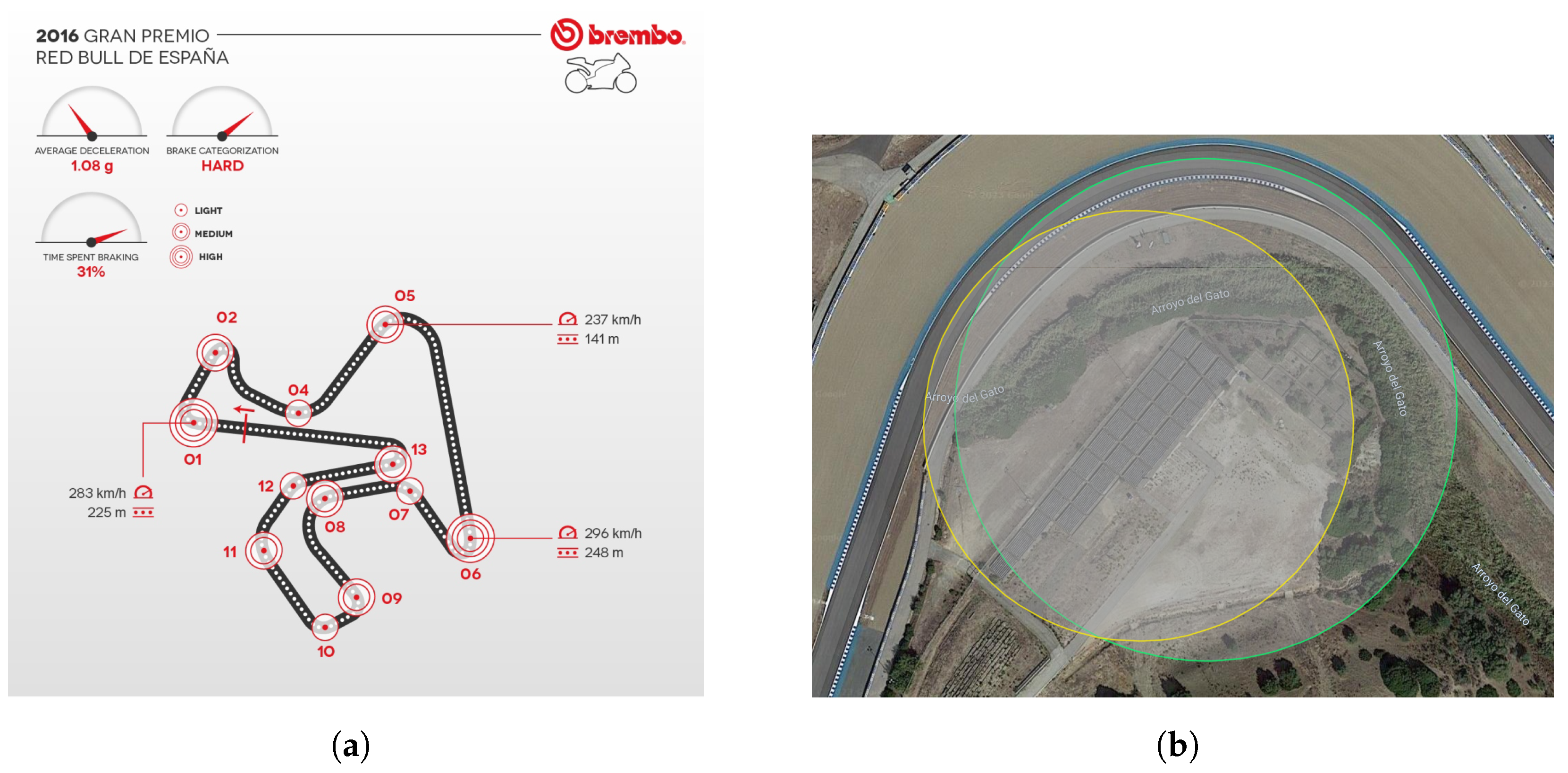
Some curves are designed for extreme braking at high speeds [13], such as the most complex braking section at the Dry Sack corner, located at Turn 6 of the Circuito Permanente MotoGP track in Spain. Riders apply more than 7.8 kg of force on the brake lever for over 5 s to decelerate from 296 $\mathrm{km}/\mathrm{h}$ to 65 $\mathrm{km}/\mathrm{h}$ (Figure 1a).

Additionally, racers can execute some curves at higher speeds without significant braking. At the Circuito Permanente track, there are four curves with radii between 20 and 30 m, three curves between 30 and 40 m, two curves between 70 and 80 m, and three more curves with radii between 80 and 115 m.

On smaller tracks, like the Euroring in Hungary, there are three curves with an approximately 15 m radius, five curves with radii between 20 and 30 m, two curves with radii between 30 and 40 m, and one with a 50 m radius.

From the curves used on racetracks and road accident data, it can be concluded that a trapezoidal membership (Equation (2)) function type may be ideal for describing the “dangerous” fuzzy set, with the following parameters (if the allowed maximum speed is higher than 50 km/h):

Risky road curvature fuzzy membership function:

$$\mu \left(risky\right)=\left\{\begin{array}{ccc}0& \mathrm{if}& x\le 20\mathrm{m}\\ (x-20)/(30-20)& \mathrm{if}& 20\mathrm{m}\le x\le 30\mathrm{m}\\ 1& \mathrm{if}& 30\mathrm{m}\le x\le 70\mathrm{m}\\ (90-x)/(90-70)& \mathrm{if}& 70\mathrm{m}\le x\le 90\mathrm{m}\\ 0& \mathrm{if}& 90\mathrm{m}\le x\end{array}\right.$$

(11)

Safe road curvature fuzzy membership function:

$$\mu \left(Safety\right)=\left\{\begin{array}{ccc}0& \mathrm{if}& x\le 80\mathrm{m}\\ (x-80)/(180-80)& \mathrm{if}& 80\mathrm{m}\le x\le 180\mathrm{m}\\ 1& \mathrm{if}& 180\mathrm{m}\le x\end{array}\right.$$

(12)

The explanation for the membership function is that curves between 20 and 30 m visually appear challenging, and drivers can visually assess their difficulty. Generally, these curves are found on winding mountain roads with fewer accelerating opportunities. However, in the case of curves with radii between 30 and 70 m on general roads with a typical speed limit of 90 $\mathrm{km}/\mathrm{h}$, accidents can easily occur if the driver does not slow down to the appropriate speed and steer the vehicle onto the correct path.

5.2. Curves with Multiple Inflection Points

Another risk factor for curves is the existence of multiple inflection points within the curve, which means that the radius of the curve can be described using multiple circles. This mainly causes two problems. One is that the drivers need to make a curve change even if they are on the correct path, and this is especially difficult when the entry speed into the curve is relatively high. The other problem is that since driving relies on everyday routine knowledge, where repetitive situations must be handled, an uncommon situation can lead to an accident. This is often the case when an animal suddenly appears on the road, thus requiring emergency braking. Therefore, emergency braking, which is not an everyday technique and can worsen the situation if executed incorrectly, is practiced in driving courses alongside simulated emergency scenarios instructing drivers on how to react when their vehicle skids in specific directions. However, changing the curve during turning, especially with a motorcycle [14], is not a simple task, and it can be considered a professional technique, especially at higher speeds, which may not be spontaneously managed by a beginner driver who has miscalculated the entry speed.

5.3. Indicating Curves with Multiple Inflection Points

Typically, dangerous curves are marked with a warning sign, but this information does not explain why the curve is dangerous. In some countries, including Hungary, road authorities are used to indicate the correct path via asphalt painting in problematic bends for motorcyclists [15]. On the Bajna–Héreg road section in Hungary, in one lane, the correct path is indicated by a green line, and in the other lane, white circles mark the path; these should be interpreted as indications to keep to the right of both the line and the circle. This serves to keep motorcyclists on the right path, but if a motorcyclist makes a mistake and drifts off course, as long as oncoming traffic follows the path specified by the markings, they are unlikely to collide. According to road authorities and the police, this type of marking has been so successful in Hungary and other countries that they plan to introduce similar markings on other dangerous curves.

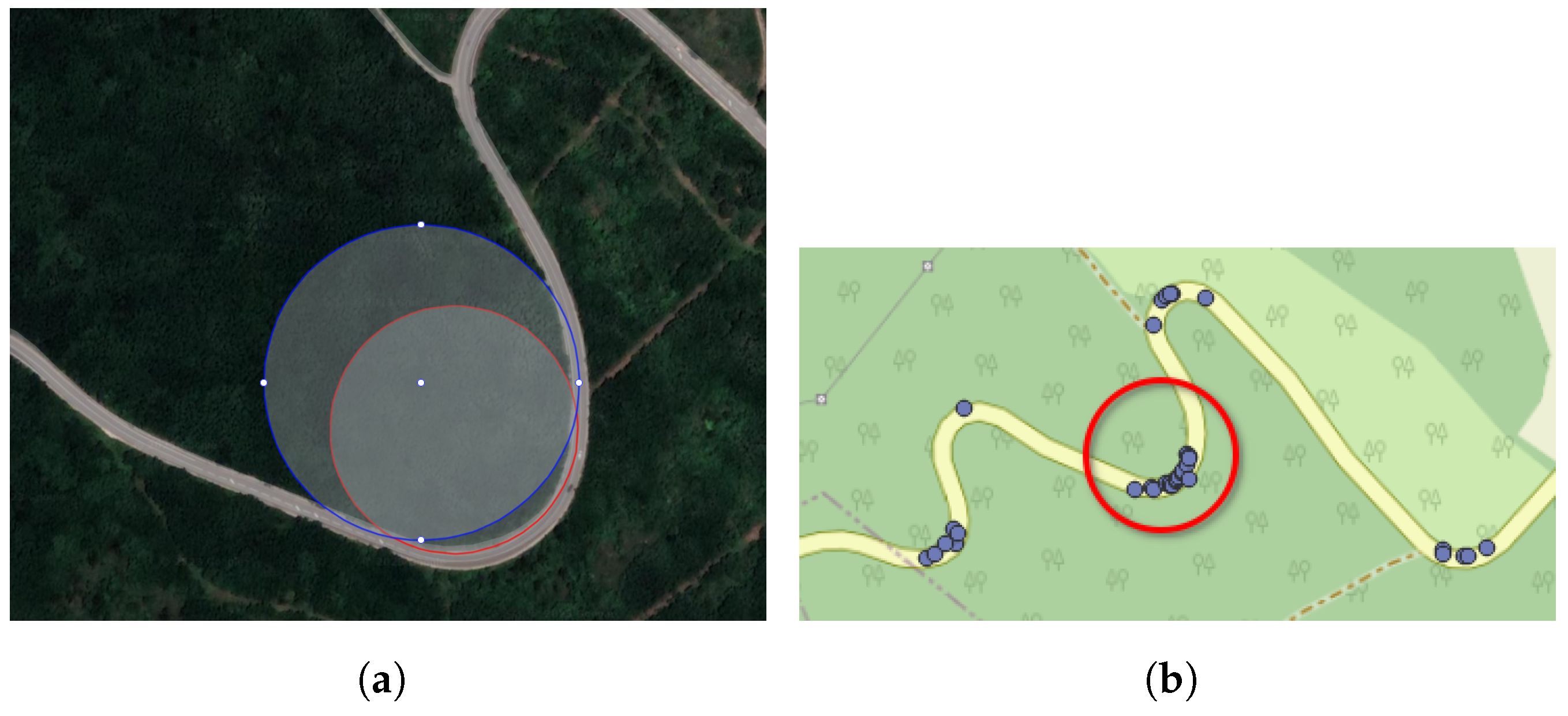
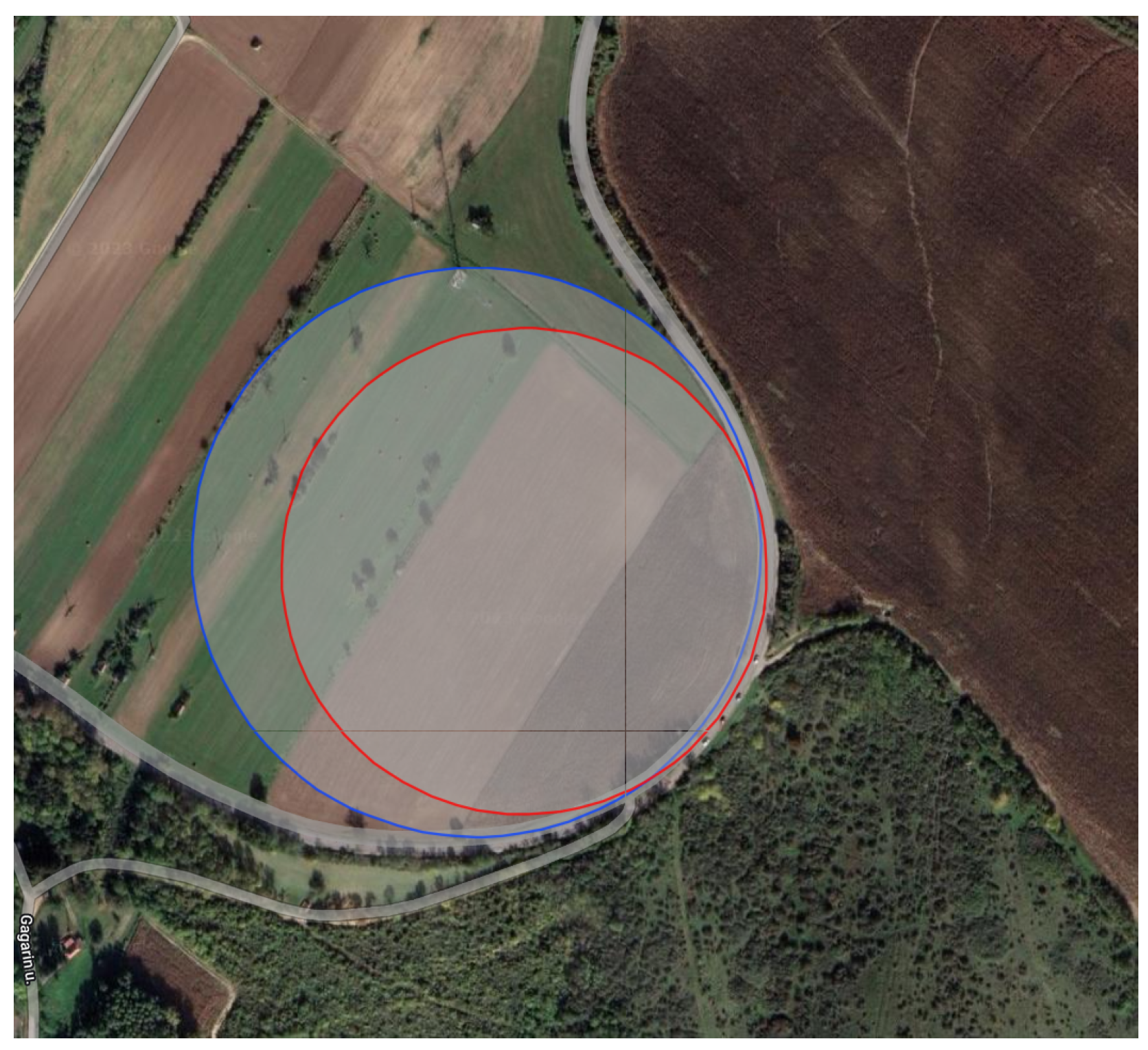
In the case of curves with multiple inflection points, the situation worsens if the visibility of the curve is low. This can be caused by changes in terrain, such as in mountainous serpentine roads, or if the curve is not very visible due to vegetation. However, even on relatively flat and sparsely vegetated terrain, curves with multiple inflection points make it harder to turn. One potential example is Road 82 in Hungary, which connects Zirc and Csesznek. According to accident statistics, most accidents are still caused by curves with multiple inflection points, but the curve itself is quite visible. It can be stated that on curves with multiple inflection points, curves with radii significantly less than 100 m pose a greater danger. This is clearly visible in the accident statistics for the Bajna–Héreg road section, and the problem can also be visually observed in Figure 2a.

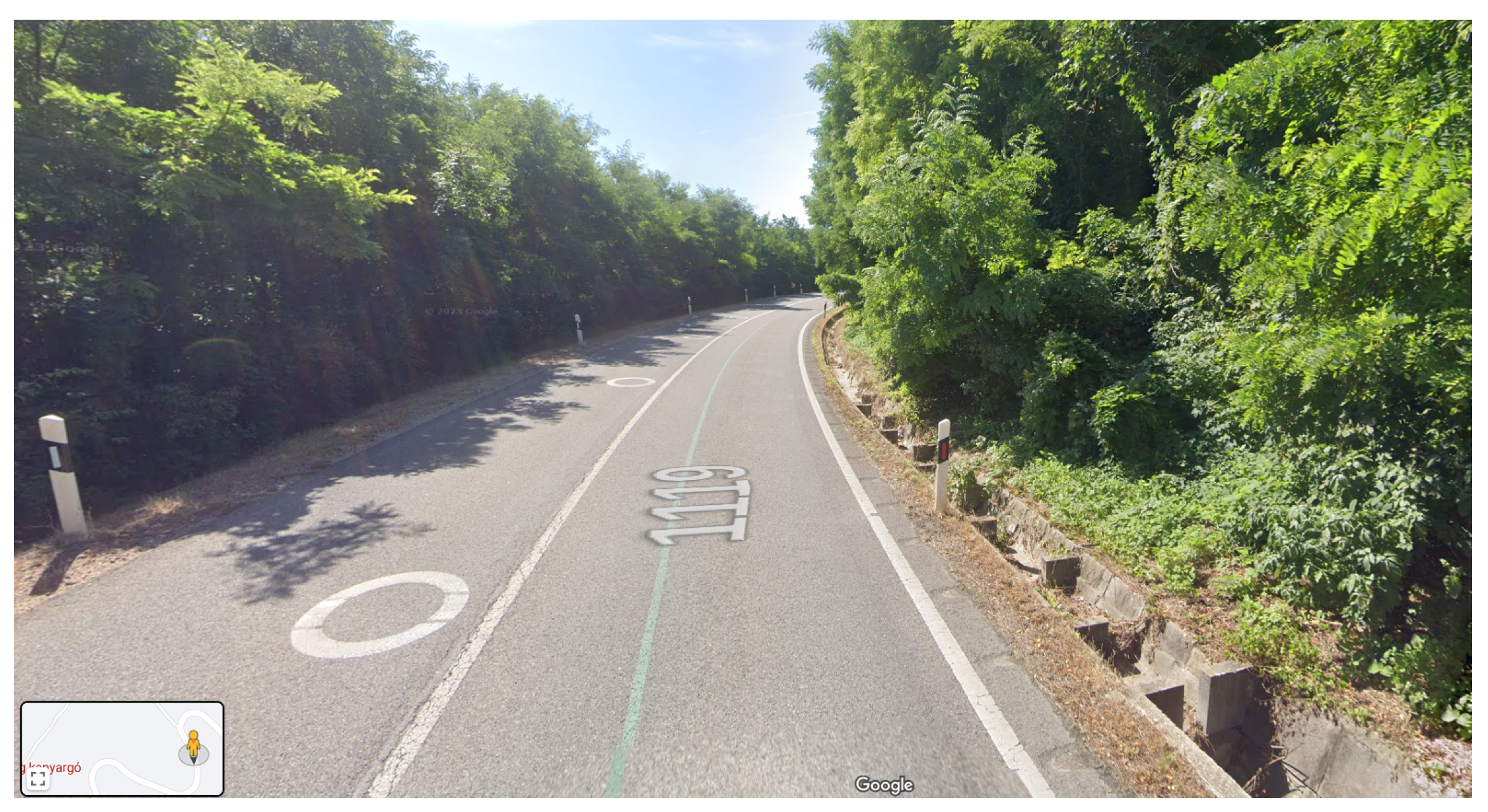
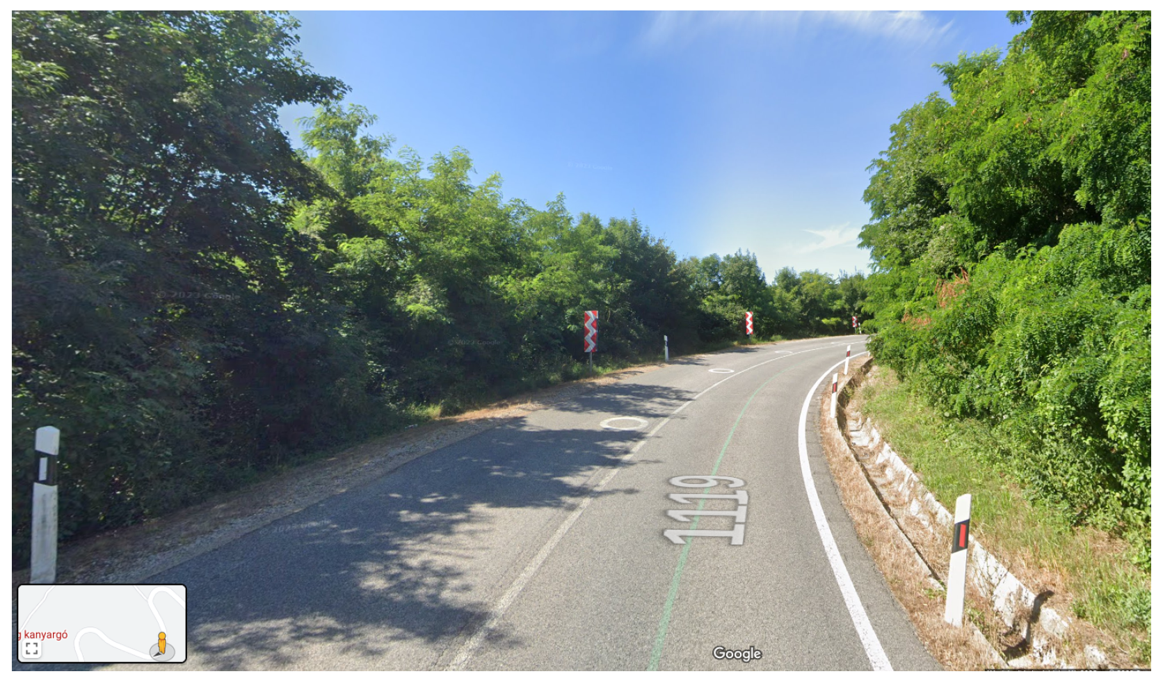
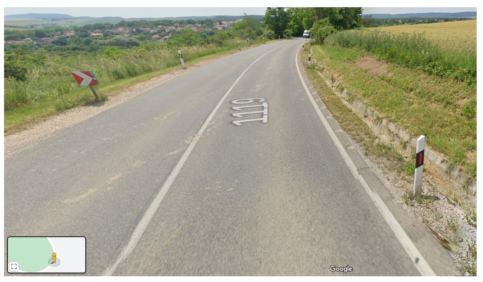
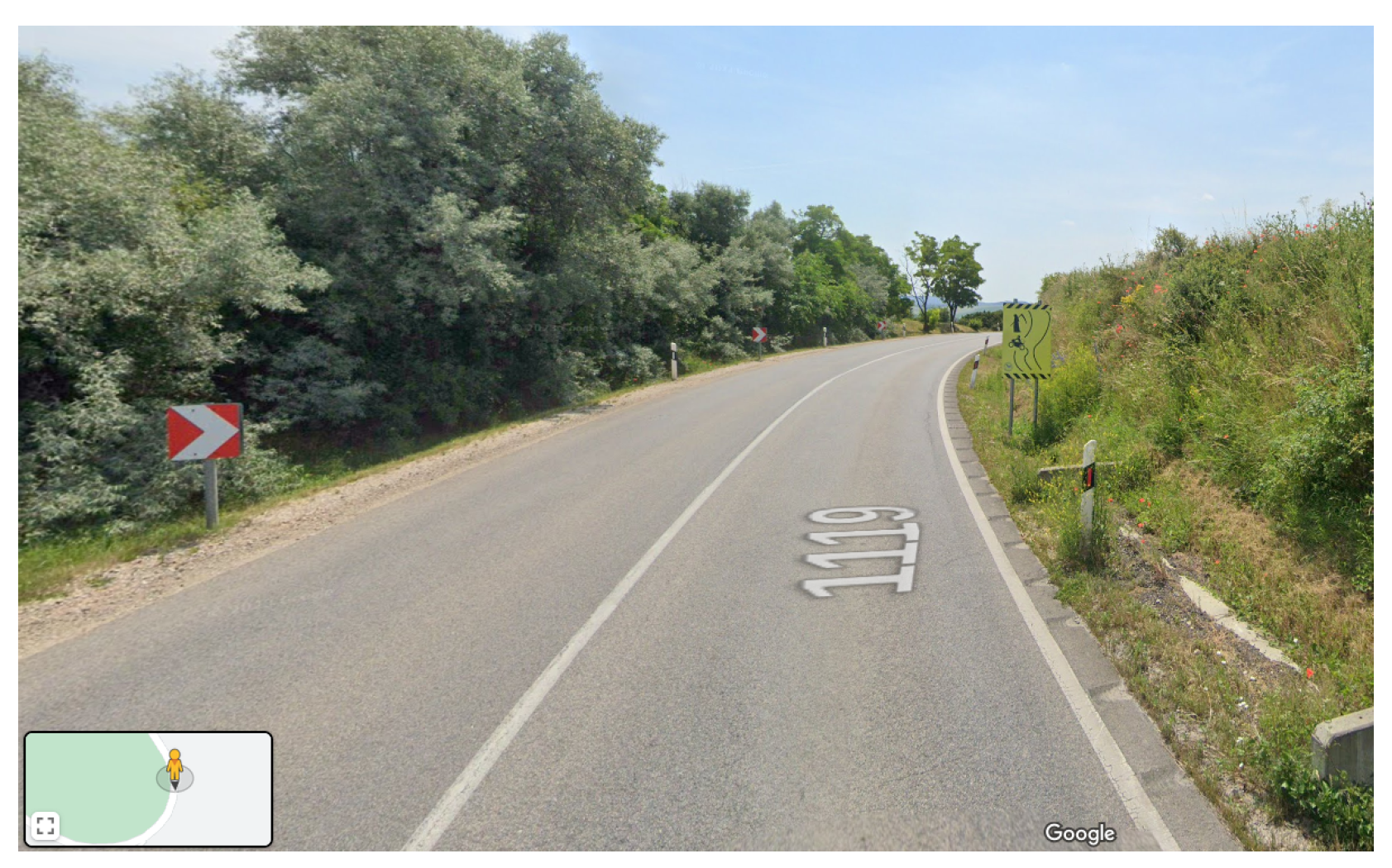
As can be seen in Figure 3, the view even gives the driver the feeling that he or she should get closer to the center line to see better. However, as seen in Figure 4, right in the middle of the curve, one must continue turning, and the curve visibility is still not high. Thus, a serious accident can occur if the driver keeps the vehicle too close to the center of the road and oncoming drivers make the same mistakes.

In the bird’s-eye view satellite image (Figure 2a), the inflection points of the curve are clearly visible, where the blue circle with a radius of approximately 78 m and the red circle with a radius of about 60 m can be observed. The situation becomes more complex due to these diameter values, as even if it were a simple 60 m or 80 m radius curve, it would still be classified as “dangerous” in the fuzzy category.

On the road leading to the town of Bajna, there is also a multi-inflection-point curve where accidents occur, but significantly fewer than on the curve between Bajna and Héreg; this is visible (Figure 5 and Figure 6) due to the fact that the diameters of the two circles that form the curve are considerably larger. The blue circle has a diameter of approximately 178 m, and the red circle is about 152 m in diameter (Figure 7).

There is an interesting curve on the Circuito Permanente MotoGP racetrack. There is also a curve that can be described by two circles (Figure 1b), but it does not intersect the other curve at the center of the turn but rather at the end. From a racing perspective, this creates an exciting turn that can be taken at high speeds. This could be a solution on public roads as well, instead of planning the inflection point at the center of the curve.

Based on accident statistical data and driving difficulty, it can be concluded that multi-radius curvature turns should be treated differently. The most common approach involves considering each turn separately, applying fuzzification to each one, as outlined in Section 5.1.

5.4. Classification of Road Slope Grade

Among the factors that increase the danger of road accidents, the slope of the road is perhaps an indicator that can be easily fuzzified in principle. Typically, road authorities use signs to indicate roads with a slope of 10% or more, drawing the attention of drivers and warning them to exercise caution. In general, for roads with a slope of 12% or more, certain practices are advisable, especially if they are exposed to more severe winter conditions. They are often made of cement because normal asphalt can melt in the summer heat. From a cyclist’s perspective [16], slopes below 8% are considered manageable, but above 8%, it becomes increasingly challenging for them. For those not cycling uphill regularly, a 12% slope is already quite difficult to manage. One of the most famous and challenging uphill sections in the Tour de France is Mont Ventoux, where the slope is 7.2% and reaches 10% in the steepest part, highlighting the difficulty of a 12% or steeper slope for cyclists. Baldwin Street in Dunedin, New Zealand, is the world’s steepest road, with a gradient of 35% over a 350 m stretch [17].

Interestingly, slopes of approximately 10% or more for vehicles can create unexpected situations similar to those faced by cyclists. It poses a physical challenge to cyclists, while for vehicles, it can reduce visibility and cause driving-related issues. For example, constant braking on a steep slope can lead to brake fluid overheating, resulting in a loss of effectiveness, which can be problematic on a winding road. Adverse weather conditions like snow or heavy rain can significantly increase road slipperiness. Additionally, the right-of-way rule can be hazardous at the intersection of streets where one or more steep streets connect. For vehicles ascending a steep slope, the driver’s attention can easily be diverted from the uphill progression.

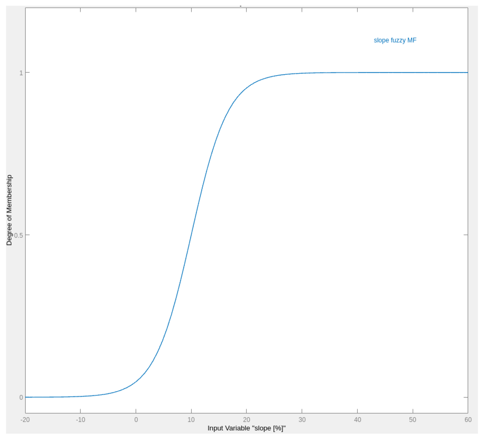
Based on the above data, two types of fuzzy membership functions can be defined: “easy” and “difficult” slopes. However, the “difficult” fuzzy set can be better described by a sigmoid (Figure 8) membership function than a trapezoidal (Equation (2)) one. The reason is that, beyond a specific value, the result is always “difficult”, unlike the “easy” fuzzy set, which is well expressed by a trapezoidal membership function.

Sigmoid difficult slope membership function (the value of x is %, indicating the road slope value):

$$sigmf(x,\alpha ,c)=\frac{1}{1+e^{-\alpha (x-c)}}$$

(13)

which is the steepness in the case of a fuzzy membership function: $\alpha =0.3$, $c=10$. In the case of the sigmoid membership function, the main criterion was to associate 10% steepness with a fuzzy value of 0.5 expressed as a percentage. The sigmoid membership function is a better choice than the trapezoid because it can cover transitions more smoothly. In determining the level of difficulty arising from changes in road steepness, this accuracy can be advantageous, even if it requires more computational effort.

Easy slope trapezoid membership function:

$$\mu \left(easy\right)=\left\{\begin{array}{ccc}0& \mathrm{if}& x\le 1\%\\ (x-1)/(3-1)& \mathrm{if}& 1\%\le x\le 3\%\\ 1& \mathrm{if}& 3\%\le x\le 6\%\\ (8-x)/(8-6)& \mathrm{if}& 6\%\le x\le 8\%\\ 0& \mathrm{if}& 8\%\le x\end{array}\right.$$

(14)

6. Fuzzy Logic-Based Rain Intensity Scaling

To determine the risk posed by the curves of a road section using a fuzzy model, it is advisable to apply slipperiness separately as a fuzzy subsystem. This subsystem calculates slipperiness based on the adhesion of the vehicle tires and the intensity of rainfall.

In the case of a road accident, apart from speeding, weather conditions often play a significant role. In driver training courses, it is a common lesson that the first fifteen minutes of rain can be quite critical and hazardous. This is because the initial rainwater mixes with the dust on the road, creating a slippery layer and making the surface considerably slick. However, after a quarter of an hour, the rain gradually washes away this layer from the asphalt. With water as a layer, the road becomes more slippery, meaning increased braking distances are required in traffic due to the risk of slipping and reduced visibility, especially as the rain intensity rises.

As the intensity of rain increases, visibility worsens, and the probability of the aquaplaning phenomenon occurring also increases. Aquaplaning occurs when there is already a significant layer of water on the road; the water fills the grooves of the car tires, which can no longer disperse it. This results in a loss of traction, as the car tires are no longer in contact with the road but rather with the water. Due to the aquaplaning phenomenon [18], the Wet Traction (WT) marking on car tires is essential, as it indicates the tire water drainage capacity [19]; this value is typically located on the sidewall of the tire.

Higher WT values signify that the tire provides a better grip on wet road surfaces, enhancing driving safety in rainy or wet weather conditions. According to the National Highway Traffic Safety Administration (NHTSA) system, the markings are as follows: “AA” for the best, “A” for better, “B” for good, and “C” for poor, representing the value ratings.

In common practice, authorities do not specify rain intensity when documenting accidents, and measuring it generally requires meteorological equipment. This is where fuzzy logic can be of assistance. In meteorology, various types of rain as precipitation have long been identified based on droplet size, and human language can distinguish between them. For example, terms such as drizzle, rain, and shower are commonly used. Meteorologically [20], drizzle is characterized by a drop diameter smaller than 1 $\mathrm{mm}$, rain has a drop diameter between 1 and 3 $\mathrm{mm}$, and the shower drop diameter is in the 3–5 $\mathrm{mm}$ range. These distinctions are perceivable by human observation and touch. Based on the diameter [21], the following fuzzy membership functions can be assigned to the types of rain:

Drizzle fuzzy membership function:

$$\mu \left(drizzle\right)=\left\{\begin{array}{ccc}0& \mathrm{if}& x\le 0.1\mathrm{mm}\\ (x-0.1)/(0.3-0.1)& \mathrm{if}& 0.1\mathrm{mm}\le x\le 0.3\mathrm{mm}\\ 1& \mathrm{if}& 0.3\mathrm{mm}\le x\le 0.8\mathrm{mm}\\ (1-x)/(1-0.8)& \mathrm{if}& 0.8\mathrm{mm}\le x\le 1\mathrm{mm}\\ 0& \mathrm{if}& 1\mathrm{mm}\le x\end{array}\right.$$

(15)

Rain fuzzy membership function:

$$\mu \left(rain\right)=\left\{\begin{array}{ccc}0& \mathrm{if}& x\le 1\mathrm{mm}\\ (x-1)/(1.5-1)& \mathrm{if}& 1\mathrm{mm}\le x\le 1.5\mathrm{mm}\\ 1& \mathrm{if}& 1.5\mathrm{mm}\le x\le 2\mathrm{mm}\\ (3-x)/(3-2)& \mathrm{if}& 2\mathrm{mm}\le x\le 3\mathrm{mm}\\ 0& \mathrm{if}& 3\mathrm{mm}\le x\end{array}\right.$$

(16)

Shower fuzzy membership function:

$$\mu \left(shower\right)=\left\{\begin{array}{ccc}0& \mathrm{if}& x\le 3\mathrm{mm}\\ (x-3)/(3.5-3)& \mathrm{if}& 3\mathrm{mm}\le x\le 3.5\mathrm{mm}\\ 1& \mathrm{if}& 3.5\mathrm{mm}\le x\le 5\mathrm{mm}\\ (7-x)/(7-5)& \mathrm{if}& 5\mathrm{mm}\le x\le 7\mathrm{mm}\\ 0& \mathrm{if}& 7\mathrm{mm}\le x\end{array}\right.$$

(17)

However, according to the NHTSA system [22], the WT value can be fuzzified.

Table 1. WT value fuzzification.

Grades	g-Force (Asphalt)	g-Force (Concrete)
AA	>0.54 g	>0.38 g
A	>0.47 g	>0.35 g
B	>0.38 g	>0.26 g
C	<0.38 g	<0.26 g

presents the NHTSA scale [23].

The “g-force” part refers to the ability of the tires to exert a force on the wet road surface that exceeds the given g-value. This means that the car tires provide enough grip on wet roads for the driver to steer and stop through the friction between the tire and the road without losing control of the vehicle. The following fuzzy membership functions are defined based on the attainable values on the asphalt:

$$\mu \left(Worsewettraction\right)=\left\{\begin{array}{ccc}1& \mathrm{if}& x\le 0.38g\\ (0.47-x)/(0.47-0.38)& \mathrm{if}& 0.38g\le x\le 0.47g\\ 0& \mathrm{if}& x>0.47g\end{array}\right.$$

(18)

$$\mu \left(Betterwettraction\right)=\left\{\begin{array}{ccc}0& \mathrm{if}& x<0.47g\\ (x-0.47)/(0.54-0.47)& \mathrm{if}& 0.47g\le x\le 0.54g\\ 1& \mathrm{if}& 0.54g<x\end{array}\right.$$

(19)

7. The Fuzzy-Based Road Accident Risk Assessment Model and Applied Methods

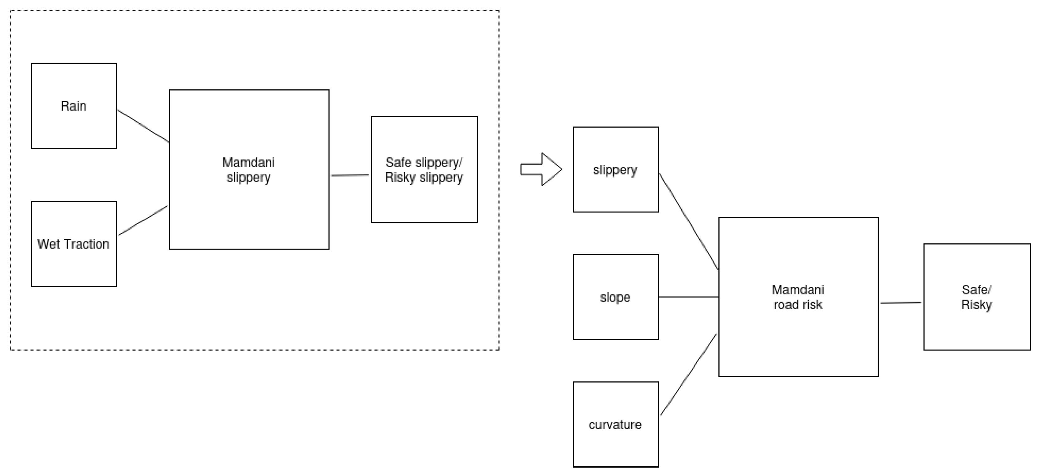
The road factors discussed in this article, such as the curve, slope, and slipperiness, can be included in a fuzzy model, as illustrated in Figure 9. Of course, the fuzzification of input values can be fine-tuned based on accident statistics reported by the country and region [24].

As mentioned in Section 6, when defining slipperiness, it is worth combining the amount of precipitation with the vehicle tire parameters. Therefore, it can be treated as a separate fuzzy subsystem, which can then provide input values to the risk-calculating fuzzy model. This is also advantageous because it keeps the system scalable.

The system rules in

Table 2. Rules of the fuzzy risk model.

	Rule
1	If slippery is safe_slip and curvature is safety_curv, then output1 is safe.
2	If slippery is safe_slip and curvature is risky_curv, then output1 is risky.
3	If slippery is risky_slip and curvature is safety_curv, then output1 is risky.
4	If slippery is risky_slip and curvature is risky_curv, then output1 is risky.
5	If slippery is safe_slip and curvature is safety_curv and slope is easy, then output1 is safe.
6	If slippery is safe_slip and curvature is safety_curv and slope is difficult, then output1 is safe.
7	If slippery is safe_slip and curvature is risky_curv and slope is easy, then output1 is risky.
8	If slippery is safe_slip and curvature is risky_curv and slope is difficult, then output1 is risky.
9	If slippery is risky_slip and curvature is safety_curv and slope is easy, then output1 is risky.
10	If slippery is risky_slip and curvature is safety_curv and slope is difficult, then output1 is risky.
11	If slippery is risky_slip and curvature is risky_curv and slope is easy, then output1 is risky.
12	If slippery is risky_slip and curvature is risky_curv and slope is difficult, then output1 is risky.
13	If slippery is risky_slip or curvature is risky_curv, then output1 is risky.
14	If slippery is risky_slip or slope is difficult, then output1 is risky.
15	If curvature is risky_curv or slope is difficult, then output1 is risky.
16	If slippery is risky_slip, then output1 is risky.
17	If slope is difficult, then output1 is risky.
18	If slippery is safe_slip and curvature is not risky_curv and slope is easy, then output1 is safe.
19	If slippery is safe_slip and curvature is not risky_curv, then output1 is safe.
20	If curvature is safety_curv, then output1 is safe.

aim to cover the classification of curve danger in slippery and steep road sections. Therefore, it is not necessary to define all the rules, but only those that are important from the perspective of curve curvature.

Both the “Slippery” and “Road risk” Mamdani models have linear Z-shaped outputs and have been defined using the “Evenly Distribute MFs” function in Matlab with the help of Fuzzy Logic Designer.

The steps of risk calculation in the model are as follows:

• Fuzzification: In the “Slippery” submodule, fuzzification is performed using (15)–(19) (see Section 6) for the inputs “Rain” and “Wet traction”. The result of this “Slippery” submodule will be one of the inputs to the “Road risk” calculation module, which also has two additional inputs: “Curvature”, whose membership functions are defined by (11) and (12), and “Slope”, whose membership functions are described by (13) and (14) (see Section 5).
• Firing strength calculation: This step uses the Zadeh t-norm and t-conorm defined by (4) and (6), respectively.
• Implication: This step uses the t-norm method defined by (4).
• Aggregation: This step uses the t-conorm method defined by (6).
• Defuzzification: The calculation is based on the CoG, defined in Section 3.4.

8. Evaluation

The secondary Hungarian road with the number 1119 is approximately 35 km long and is located in Komárom-Esztergom county. It serves as one of the most important secondary roads in the county, providing a direct connection between the county seat, Tatabánya, and the areas of Esztergom and Dorog. Its main direction is generally southwest, but the orientation varies on different sections due to the topography. Based on accident statistics, the section between Bajna and Héreg experiences the highest frequency of accidents. This particular section can serve as a valuable test case for evaluating the model classification of dangerous curves, as outlined in Section 7.

8.1. Evaluation Using the Proposed Model

For verification, the section between Bajna and Nagysáp can be examined using the model, as this segment experiences fewer accidents and features a similarly winding road.

The radii of the curves of the two examined sections and the risk values calculated by the fuzzy system in Section 7 are presented in

Table 3. Curvature between Bajna and Héreg.

1119 Bajna–Héreg Curvature	Fuzzy Risk Factor	Number of Accidents
86 m	0.345	7
67 m	0.75	7
49 m	0.75	6
78 m/60 m (multi-radius)	0.551/0.75	24
57 m	0.75	1
59 m	0.75	6
118 m	0.264	3
87 m	0.322	2
57 m	0.75	10

and

Table 4. Curvature between Bajna and Nagysáp.

1119 Bajna–Nagysáp Curvature	Fuzzy Risk Factor	Number of Accidents
238 m	0.252	0
204 m	0.252	2
201 m	0.252	4
156 m	0.264	2
152 m/178 m (multi-radius)	0.264/0.253	7
189 m	0.251	2

.

Based on the tables, it can be concluded that the section between Bajna and Héreg is indeed more risky than the segment between Bajna and Nagysáp. The average risk value for Bajna–Héreg is 0.598, while Bajna–Nagysáp averages 0.292. Interestingly, both cases involve multi-radius curves on the road, but in the case of the Bajna–Nagysáp route, larger-radius circles form the curves, making them less dangerous. Regarding the number of accidents, there were 66 accidents in the Bajna–Héreg section between 2017 and 2022, while the Bajna–Nagysáp section had 17 accidents during the same period.

Since accidents occurred in both dry and rainy weather, but the official data do not cluster rain separately, and modern vehicle tires mostly have good Wet Traction (WT) values (“A”), the danger of curves was calculated with a 0.2 slipperiness value. Furthermore, the 1119 road has a slope value of 0.

8.2. Comparison of Fuzzy Model Results with WOM and Heatmap Results

As mentioned in Section 4, Aslam Al-Omari et al. [11] compared the results of the fuzzy-based (FOM) method with the Weighted Overlay Method (WOM) in the analysis of hazardous road sections. Since these methods produce visually evident results, it is interesting to compare the results of the fuzzy model with heatmap and WOM analyses.

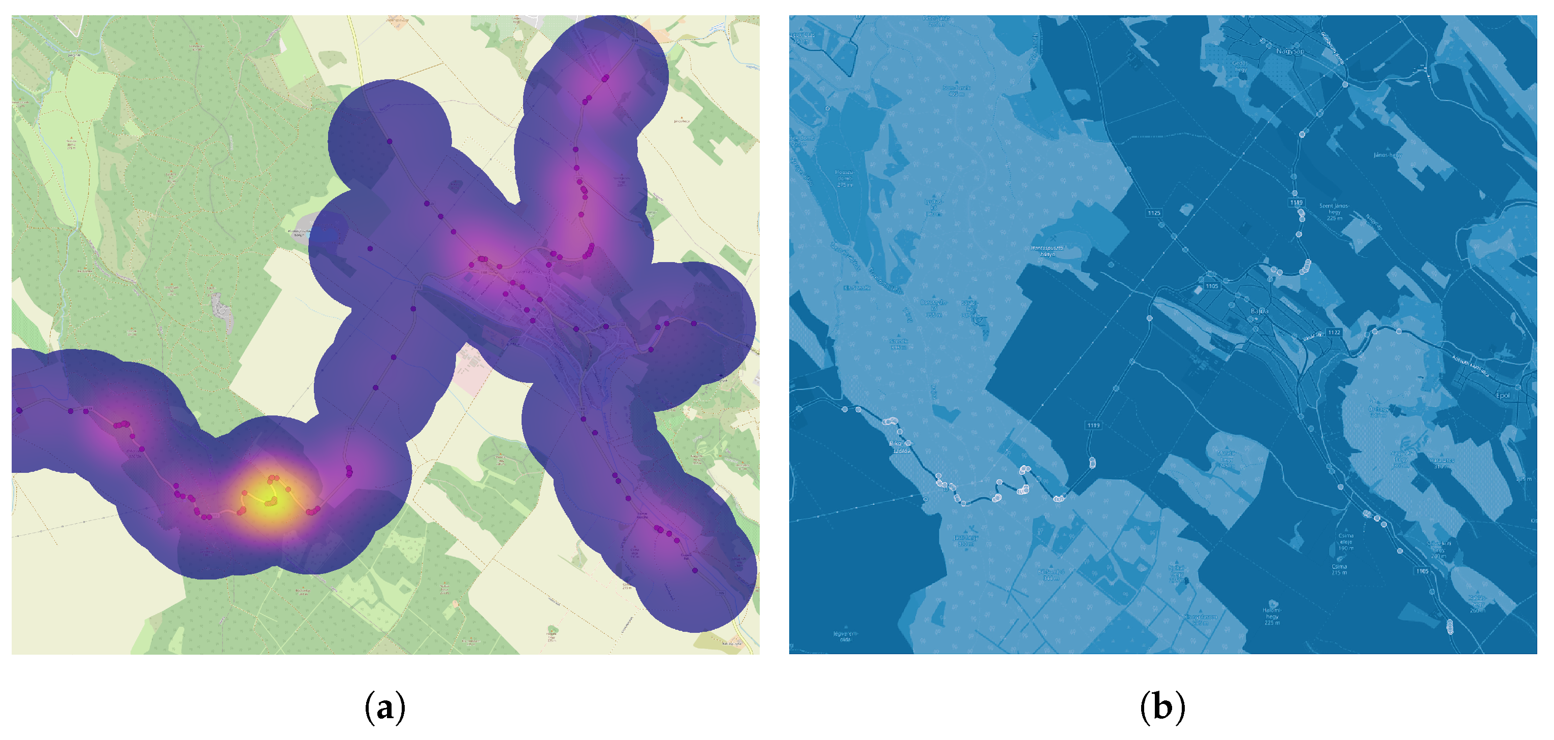
The heatmap and WOM images (Figure 10) clearly show that both methods highlight the sections along the analyzed route where the fuzzy model introduced in this article indicates higher risk.

In QGIS software, it is possible to conduct heatmap and WOM analyses. The Heatmap plugin employs Kernel Density Estimation to generate a density (heatmap) raster from an input point vector layer. The density is computed by considering the number of points in a specific location, where higher concentrations of clustered points correspond to elevated values. The Kernel Density Estimation (KDE) heatmap estimates the density or probability of spatial points based on a given dataset. KDE is a smoothing technique commonly expressed through the following formula:

$$f\left(x\right)=\frac{1}{nh}\sum _{i=1}^{n}K\left(\frac{x-x_i}{h}\right)$$

(20)

• n is the number of data points in the dataset.
• K is the kernel function, which is a smoothing function. The most commonly used kernel functions are the Gaussian (normal) and Epanechnikov kernels.
• h is the smoothing parameter or bandwidth, which determines how smooth the estimation should be.

Heatmaps facilitate the straightforward identification of “hotspots” and the visualization of point clustering.

The Epanechnikov kernel function (21) was chosen because it can perform better on datasets where the majority consists of smaller values, and outliers are less important.

Epanechnikov kernel function:

$$P_x=\frac{3}{4}(1-d^2)$$

(21)

The WOM analysis was performed by exporting accidents that occurred on curves with radii smaller than 80 m and those with radii greater than 80 m as separate layers within the studied area. Additionally, accidents on slopes and during rainy conditions were exported into distinct layers. Weighting was performed with a weight of 0.65 assigned to accidents on curves smaller than 80 m, as 65% of the accidents occurred on such curves. The slope layer was given a weight of 0.2 because 22% of the accidents occurred on slopes, and accidents during rainy conditions were assigned a weight of 0.13, as 13% of the accidents occurred in rainy weather.

8.3. Comparative Discussion

Table 5. KDE heatmap results.

1119 Bajna–Héreg Curvature	KDE Heatmap Concentration Value	Fuzzy Risk Factor	Accidents
86 m	10.8	0.345	7
67 m	20.5	0.75	7
49 m	22.9	0.75	6
78 m/60 m	30.8	0.551/0.75	24
57 m	22.5	0.75	1
59 m	22.5	0.75	6
118 m	10.2	0.264	3
87 m	10.8	0.322	2
57 m	14.4	0.75	10

is a comparative table that numerically and visually compares the fuzzy-based model presented in this paper with the KDE-based heatmap method. It is compared to the KDE-based heatmap method because it presents the results both numerically and visually.

As visually depicted in Figure 10a, the KDE heatmap and WOM results clearly show the more dangerous sections of the road; however, they do not provide enough details about the differences in the hazard between curves, making it challenging to rank them, unlike the fuzzy model results. As seen in Table 5, it does not indicate the correlation between the heatmap concentration value and the radius of the curvature value.

Furthermore, as indicated by Table 5, the fuzzy-based model can more accurately indicate the level of danger and correct the error resulting from the inaccuracy of accident coordinates. In the last row of Table 5, for a curve with a radius of 57 m, the fuzzy-based model calculated a risk factor of 0.75, and there were 10 accidents recorded between 2017 and 2022. However, the concentration value of the heatmap is only 14.4 (with 30.8 being the highest concentration), indicating that the accident coordinates are not concentrated enough. The novelty of the method described in this article is that it can more accurately identify dangerous accident spots than a KDE-based heatmap. Additionally, due to its hierarchical structure, it can be further expanded in the future by considering other factors.

9. Conclusions

In traffic, one of the main goals is to ensure the highest possible safety for all participants. For this purpose, a given route must be planned and implemented as safely as possible, considering its environment’s characteristics. The sections covered in this article have served as a basis for classifying rain, curves, combinations of curves, and slopes in a fuzzy-based scale system. This allows their incorporation into a more complex fuzzy system, enabling the fuzzy-based risk classification of a given road section. The model presented in this article works well primarily for assessing the risk of winding road sections.

This can be useful because certain route planning software [8] considers traffic conditions and may also consider a road section to be more risky in the rain than in good weather.

10. Future Research

Given the hierarchical structure of the system, expanding the subsystems allows for the scalability of the model, facilitating easy future enhancements.

The aim of future research will be to improve the model presented in this article with additional fuzzy subsystems based on the accident databases of several countries to more accurately estimate risk. As a fuzzy subsystem, daily traffic clustering could expand because, in cities, certain intersections are more dangerous during busy periods than during less busy times.

References

- Clarke, D.D.; Ward, P.; Bartle, C.; Truman, W. The role of motorcyclist and other driver behaviour in two types of serious accident in the UK. Accid. Anal. Prev. 2007, 39, 974–981. [Google Scholar] [CrossRef] [PubMed]
- Li, A.Z.; Song, X.H. Traffic accident characteristics analysis based on fuzzy clustering. In Proceedings of the 2012 IEEE Symposium on Electrical & Electronics Engineering (EEESYM), Kuala Lumpur, Malaysia, 24–27 June 2012; pp. 468–470. [Google Scholar]
- Skorupski, J. The simulation-fuzzy method of assessing the risk of air traffic accidents using the fuzzy risk matrix. Saf. Sci. 2016, 88, 76–87. [Google Scholar] [CrossRef]
- Stanković, M.; Stević, Ž.; Das, D.K.; Subotić, M.; Pamučar, D. A new fuzzy MARCOS method for road traffic risk analysis. Mathematics 2020, 8, 457. [Google Scholar] [CrossRef]
- Wang, H.; Zheng, L.; Meng, X. Traffic Accidents Prediction Model based on Fuzzy Logic, Proceedings of the Advances in Information Technology and Education: International Conference, CSE 2011, Qingdao, China, 9–10 July 2011; Proceedings, Part I. Springer: Berlin/Heidelberg, Germany, 2011; pp. 101–108.
- Liu, Y.; Huang, X.; Duan, J.; Zhang, H. The assessment of traffic accident risk based on grey relational analysis and fuzzy comprehensive evaluation method. Nat. Hazards 2017, 88, 1409–1422. [Google Scholar] [CrossRef]
- WHO. Estimated Number of Road Traffic Death. Technical Report. 2021. Available online: https://www.who.int/data/gho/data/indicators/indicator-details/GHO/estimated-number-of-road-traffic-deaths (accessed on 27 February 2024).
- Xie, B.; Zheng, H.; Ma, H. Fuzzy-logic-based traffic incident detection algorithm for freeway. In Proceedings of the 2008 International Conference on Machine Learning and Cybernetics, Kunming, China, 12–15 July 2008; Volume 3, pp. 1254–1259. [Google Scholar]
- Loukas Dimitriou, E.I. Fuzzy modeling of freeway accident duration with rainfall and traffic flow interactions. Anal. Methods Accid. Res. 2015, 5–6, 59–71. [Google Scholar] [CrossRef]
- Ali, F.; Ali, A.; Imran, M.; Naqvi, R.A.; Siddiqi, M.H.; Kwak, K.S. Traffic acciden detection and condition analysis based on social neworking data. Accid. Anal. Prev. 2021, 151, 105973. [Google Scholar] [CrossRef] [PubMed]
- Al-Omari, A.; Shatnawi, N.; Khedaywi, T.; Miqdady, T. Prediction of traffic accidents hot spots using fuzzy logic and GIS. Appl. Geomat. 2020, 12, 149–161. [Google Scholar] [CrossRef]
- Milleville-Pennel, I.; Jean-Michel, H.; Elise, J. The use of hazard road signs to improve the perception of severe bends. Accid. Anal. Prev. 2007, 39, 721–730. [Google Scholar] [CrossRef] [PubMed]
- Brembo. An In-Depth Look at the Premier Class’ Use of the Braking Systems on the Jerez Circuit; Technical Report; Brembo: Curno, Italy, 2016. [Google Scholar]
- Clarke, D.D.; Ward, P.; Bartle, C.; Truman, W. In-Depth Study of Motorcycle Accidents; Road Safety Research Report No. 51; Department for Transport: London, UK, 2004.
- Biral, F.; Bosetti, P.; Lot, R. Experimental evaluation of a system for assisting motorcyclists to safely ride road bends. Eur. Transp. Res. Rev. 2014, 6, 411–423. [Google Scholar] [CrossRef]
- De Neef, M. Gradients and Cycling: An Introduction. 2013. Available online: https://theclimbingcyclist.com/gradients-and-cycling-an-introduction/ (accessed on 27 November 2023).
- Guiness World Records. Baldwin Street in New Zealand Reinstated as the World’s Steepest Street. 2020. Available online: https://www.guinnessworldrecords.com/news/2020/4/baldwin-street-in-new-zealand-reinstated-as-the-worlds-steepest-street-614287 (accessed on 27 November 2023).
- Mouri, H.; Akutagawa, K. Improved tire wet traction through the use of mineral fillers. Rubber Chem. Technol. 1999, 72, 960–968. [Google Scholar] [CrossRef]
- Tuononen, A.J.; Matilainen, M.J. Real-time estimation of aquaplaning with an optical tyre sensor. Proc. Inst. Mech. Eng. Part D J. Automob. Eng. 2009, 223, 1263–1272. [Google Scholar] [CrossRef]
- Yuter, S.E.; Kingsmill, D.E.; Nance, L.B.; Löffler-Mang, M. Observations of precipitation size and fall speed characteristics within coexisting rain and wet snow. J. Appl. Meteorol. Climatol. 2006, 45, 1450–1464. [Google Scholar] [CrossRef]
- Bourgouin, P. A method to determine precipitation types. Weather. Forecast. 2000, 15, 583–592. [Google Scholar] [CrossRef]
- U.S. Department of Transportation. Consumer Guide to Uniform Tire Quality Grading; Technical Report; U.S. Department of Transportation: Wasington, DC, USA, 2015.
- Legal Information Institute. 49 CFR § 575.104—Uniform Tire Quality Grading Standards; Technical Report; Legal Information Institute: Ithaca, NY, USA, 1978. [Google Scholar]
- Abdullah, L.; Zamri, N. Road traffic accidents models using threshold levels of fuzzy linear regression. In Proceedings of the 2012 International Conference on Statistics in Science, Business and Engineering (ICSSBE), Langkawi, Malaysia, 10–12 September 2012; pp. 1–5. [Google Scholar]