1. Introduction
As is widely known, nonlinear system control is an important topic of control fields, especially for discrete-time nonlinear systems, and is difficult for traditional control methods. In recent decades, many different approaches to discrete-time system control have been proposed, such as adaptive control [
1], fuzzy control [
2], and PID control [
3]. Optimal tracking control, one of the effective methods for nonlinear systems, has many practical engineering applications [
4,
5,
6]. Its purpose is to design a control law that not only allows the system to track the desired trajectory but also minimizes a specific performance index. It is of great theoretical significance to explore the optimal tracking optimal control of nonlinear systems. Although dynamic programming is an effective method for solving optimal control problems, there is the problem of “curse of dimensionality” when dealing with relatively complex systems [
7,
8]. Moreover, it is difficult to solve the HJB equation derived from the optimal control of nonlinear systems, which has no analytical solution.
On the other hand, neural network control is used as a common control method for uncertainly nonlinear systems. In 1990, Narendra et al. first proposed an artificial neural network (ANN) adaptive control method for nonlinear dynamical systems [
9]. Through neural network approximation, the uncertain system can be reconstructed using input and output data. Since then, multilayer neural networks (MNNs) have been successfully applied in pattern recognition and control systems [
10]. This also has led to the generation of many types of neural networks, including the RBF-NN. In [
11], Poggio et al. first proved that the RBF-NN is superior in approximating functions. Studies of RBF-NNs have also shown that these neural networks have the ability to approximate any nonlinear function with a compact ensemble and arbitrary accuracy [
12,
13]. Compared to other ANNs, the RBF-NN does not have the complex structure of neural networks such as back propagation (BP) networks or recurrent neural networks (RNNs), and it is easier to select parameters [
11,
14,
15]. Its good generalization ability, simple network structure, and avoidance of unnecessarily lengthy computations are advantages that make RBF-NNs attract attention [
15,
16]. Many research results have been published on neural network control for nonlinear systems [
17,
18,
19].
Benefiting from neural networks and reinforcement learning (RL), the difficult problem of solving nonlinear HJB partial differential equations is solved. The ADP algorithm was proposed by Powell to approximate the solution of the HJB equation [
20], which combines the theory and methods of RL, neural networks, adaptive control and optimal control. As developed, ADP has not only been considered as one of the core methods for solving the diversity of optimal control problems but also has been successfully applied to both continuous-time systems [
21,
22,
23] and discrete-time systems [
24,
25,
26,
27,
28,
29,
30,
31] to search for solutions of the HJB equations online. Particularly, several works have attempted to solve the discrete time nonlinear optimal regulation problem using the ADP algorithm such as robust ADP [
32,
33,
34,
35], iterative/invariant ADP [
36,
37,
38,
39], off-policy RL [
40,
41,
42] and the Q-Learning Algorithm [
40,
43].
In the past decades, many relevant studies have been conducted on the optimal tracking control of discrete-time nonlinear system using the ADP algorithm. However, in the existing literature on optimal tracking of nonlinear discrete-time systems, there is no RBF neural network-based ADP algorithm. In this paper, an optimal tracking control method based on RBF-NNs for discrete-time partially unknown nonlinear systems is proposed. Two RBF neural networks are used to approximate the unknown system dynamic as well as the steady-state control. After transforming the tracking problem into a regulation problem, the critic network and the actor network are used to obtain the nearly optimal feedback control, which allows the online learning process to require only current and past system data.
The contributions of article are as follows: (1) Unlike the classical technique of NN approximation, we propose a near-optimal tracking control scheme for a class of partially unknown discrete-time nonlinear systems based on RBF-NNs and prove the stability of the system. (2) Compared with [
35,
39], we additionally used an RBF-NN to directly approximate the steady-state controller of the unknown system. It can solve the requirement for the priori knowledge of the controlled system dynamics and reference system dynamics. Moreover, we propose a novel adaptive law to update the weight of the steady-state controller.
The paper is organized as follows. The problem statement is shown in
Section 2. The design of the optimal tracking controller of the system with partially unknown nonlinear dynamics is given in
Section 3, which includes the RBF-NN identifier, the RBF-NN steady-state controller, near optimal feedback controller, and stability analysis.
Section 4 provides simulation results to validate the proposed control method and details the method comparison.
Section 5 draws some conclusions.
2. Problem Statement
Consider the following affine nonlinear discrete-time system [
31]:
where
is the measurable system state and
is the control input. Assume that the nonlinear smooth function
is an unknown drift function,
is a known function, and
where the Frobenius norm
is applied. In addition, assume that
has a generalized inverse matrix
such that
where
I is the identity matrix. Let
be the initial state.
The reference trajectory is generated by the following bounded command:
where
and
, and
is the reference trajectory; it need only be a stable state trajectory or asymptotically stable.
The goal of this paper is to design a controller
that not only ensures the state of the system (
1) tracks the reference trajectory but also minimizes a cost function. For the optimal tracking control technique, the cost functions are usually considered in quadratic form [
4], that is
where
and
are symmetric positive definite;
is tracking error. For common solutions of tracking problems, the control input consists of two parts, a steady-state input
and a feedback input
[
24]. Next, we will discuss how to obtain each part.
The steady-state controller is used to ensure perfect tracking. This perfect tracking equation is realized under the condition
. For this condition to be fulfilled, the steady-state part of the control
must exist to make
equivalent to
. By substituting
and
into system (
1), the reference state is
where
and
are bounded to be tracked by the reference trajectory. If the system dynamics (
1) are known,
is acquired by
where
is the generalized inverse of
with
.
Remark 1. In the subsequent discussion, the RBF network can be used to identify the unknown dynamics of system (1); hence, (5) can be computed. By using (
1) and (
4), the tracking error dynamics
are given by
where
,
, and
.
is the feedback control input. By minimizing the cost function, it is designed to stabilize the tracking error dynamics. For
in the control sequence, the cost function can be expressed as the following discrete time tracking HJB equation
where
,
for
and
,
denotes the cost function at the next tracking error dynamics
. The tracking error
is used in the study of the cost function of the optimal tracking control problem.
In general, this feedback control
is found by minimizing (
7) to solve the extremum condition in the optimal control framework [
4]. This result is
Then, the standard control input is obtained
where
is obtained from (
5), and
is obtained from (
8).
As detailed in the subsequent discussion, in order to acquire the unknown dynamics in system (
1), we used the RBF neural networks to reconstruct system dynamics. Moreover, faced with the problem of unable to find the analytical solution of (
7) and the curse of dimensionality, the ADP algorithm was used to approximately solve the HJB Equation (
7).
The main results of this paper are based on the following definitions and assumptions [
30].
Definition 1. A control law is admissible with respect to (7) on the set Ω if is continuous on a compact set for , , and is finite. Assumption 1. System (1) is controllable, and the system state is in equilibrium under control . Input control satisfies for , and the cost function is a positive definite function for any and . Lemma 1. For the tracking error system (6), assume that is an admissible control, the internal dynamics is bounded, andwhere is the minimum eigenvalue of R, is the minimum eigenvalue of Q, and is a known positive constant. Then, the tracking error system (6) is asymptotically stable. Proof. We consider the following Lyapunov function,
where
is defined in (
7). Differencing the Lyapunov function yields
Using (
6) and (
7), we can obtain
Using the Cauchy–Schwarz inequality yields
For the purpose of asymptotically stabilizing the tracking system (
6), i.e.,
, it is necessary to satisfy the following
Thus,
and the asymptotic stability of the tracking error system (
6) are proved if the bound in (
10) is satisfied. □
Remark 2. Lemma 1 shows that under the condition that the internal dynamics is bounded to satisfy (10), there exists an admissible control that not only stabilizes the tracking error system (6) on Ω but also guarantees that the cost function is finite. 3. Optimal Tracking Controller Design with Partially Unknown Dynamics
In this section, firstly, we use an RBF-NN to approximate the unknown system dynamics and use another RBF-NN to approximate the steady-state controller . Secondly, two feedback neural networks are introduced to approximate the cost function and the optimal feedback control . Finally, the system stability is proved by selecting an appropriate Lyapunov function.
3.1. RBF-NN Identifier Design
In this subsection, in order to capture the unknown dynamics of the system (
1), an RBF-NN-based identifier is proposed. Without losses of generality, this unknown dynamics is assumed to be a smooth function within a compact set. Using an RBF-NN, this unknown dynamics (
1) is identified as
where
is the matrix of ideal output weights of the neural network and
is the vector of radial basis functions,
is the bounded approximation error, and
, where
is a positive constant.
For any non-zero approximation error
, there exists optimal weight matrix
such that
where
is the optimal weight of identifier, and
. The output weights are updated, and the hidden weights remain unchanged when training, so the neural network model identification error is
where
.
The error function is defined as the following
Using the gradient descent method, the weights are updated by
and
where
is the learning rate of the identifier.
Inspired by the work in [
36], we must state the following assumptions before proceeding.
Assumption 2. The neural network identifying error is assumed to have an upper bound, namely 3.2. RBF-NN Steady-State Controller Design
We use the RBF-NN to approximate the steady-state control
directly, and the inverse dynamic NN is established to approximate [
16,
19].
We design the steady-state control
through the approximation of the RBF-NN
where
is the actual neural network weights;
is the output of the hidden layers; and
is the output of the RBF-NN.
Let the ideal steady-state control
be
where
is the optimal neural network weights and
is the error vector. Assuming that
is the reference output of the system at the point
, without considering external disturbances, the control input
satisfies
where
.
Thus, we can define the error
of the approximation state as
where
.
(
24) subtracted from (
23) yields
where
is weight approximation error.
The weights are updated by the following update law of the weights
where
and
are the positive constant.
Assumption 3. Within the set , the optimal neural network weights and the approximation error are bounded. 3.3. Near-Optimal Feedback Controller Design
In this subsection, we present an ADP algorithm based on the Bellman optimality. The goal is to find the optimal approximate feedback control law that minimizes the approximate cost function.
First, considering the HJB Equation (
7) and the optimal feedback control (
8), the cost function
is rewritten as
. The initial cost function
may not represent the optimal value function. Then, a single control vector
can be solved by
Updating the control law yields
Hence, for
, the ADP algorithm can be realized in a continuous iterative process in
and
where index
i represents the number of iterations of the control law and the cost function, i.e., the update count of internal neuron to update the weight parameters, while index
k represents time index of state. Moreover, it is worth noting in the iterative process of the ADP algorithm that the number of iterations of the cost function and the control law increases from zero to infinity.
To begin the development of the feedback control policy, we used neural networks to construct the critic network and the actor network.
The cost function is defined as the critic network.
The output of the critic network is denoted as
where
is the hidden layer function,
is the hidden layer weight of the critic network,
is the input layer weight of the critic network, and
is the approximation error.
So, we define the prediction error of the critic network as
The error function of the critic network is defined as
Using the gradient descent method, the weights of the critic network are updated,
where
is the learning rate of the critic network.
The inputs of the actor network is the system error
, and the outputs of the actor network is the optimal feedback control
. The output can be formulated as
where
is the hidden layer function,
is the hidden layer weight of the actor network,
is the input layer weight of the actor network, and
is the approximation error.
Similar to the critic network, the prediction error of the actor network is defined as
where
is approximation optimal feedback control, and
is the optimal feedback control at the iterative number
i.
The error function of the actor network is defined as
The weights of the actor network are also updated in the same way as the critic network; we use the gradient descent method
where
is the learning rate of the actor network, and
i is the update count of the internal neuron to update the weight parameters.
3.4. Stability Analysis
In this subsection, we give the stability proof by Lyapunov’s stability theory.
Assumption 4. Radial basis function of the maximum value is , where is the center point and b is the width of radial basis function. Assuming the numbers of neurons is for any radial basis function , thenWe can know the maximum value of the hidden layer with l neurons is , then we assume the maximum value of the hidden layer for the identifier is , and the maximum value of the hidden layer for the steady-state controller is . Lemma 2. The relationship between (25) and weight approximation error (27) satisfies the following equation.where is the error of the approximation state , , , and ϵ are positive constants. Proof. Subtracting
from both sides of (
28), we obtain
Combining (
25) and (
27) with the mean value theorem, we can obtain
Further combining (
45) with (
26), we can obtain
After rearranging, we can obtain
The proof is completed. □
Lemma 3. For simplicity of analysis, and have an inequality relation though using Assumption 3 and Young’s inequality.where is a positive constant. Theorem 1. For the optimal tracking problem (1)–(3), the RBF-NN identifier (16) is used to approximate , the steady-state controller is approximated by the RBF-NN (23), and the feedforward networks (34), (38) are used to approximate the cost function and the feedback controller , respectively. Assume that the parameters satisfy the following inequalitywhere η is the learning rate of the RBF-NN identifier, σ and γ are the update parameters of the steady-state controller approximation network weights, is the learning rate of the actor network, is the learning rate of the critic network, and and are hidden layer functions of the actor network and the critic network. Then, the closed loop system (6) of approximation error is asymptotically stable when the parameter estimation errors are bounded. Proof. Considering the following positive definite Lyapunov function candidate
where
,
,
,
.
Firstly, differencing it according to the Lyapunov function of
yields
According to the Assumption 2, Assumption 4 and (
42), (
51) can be carried out to obtain
Next, differencing according to the Lyapunov function of
yields
where
Considering (
26) and
, we can deduce
Recall Lemmas 2 and 3; substituting (
54) into (
53) yields
where
is a positive constant.
Next, we consider the following Lyapunov function
Then, differencing it according to the Lyapunov function of (
57) yields
Finally,
is derived from (
52), (
56), and (
58)
Based on the above analysis, when the parameters are selected to fulfill the following condition with
,
we can obtain
. □
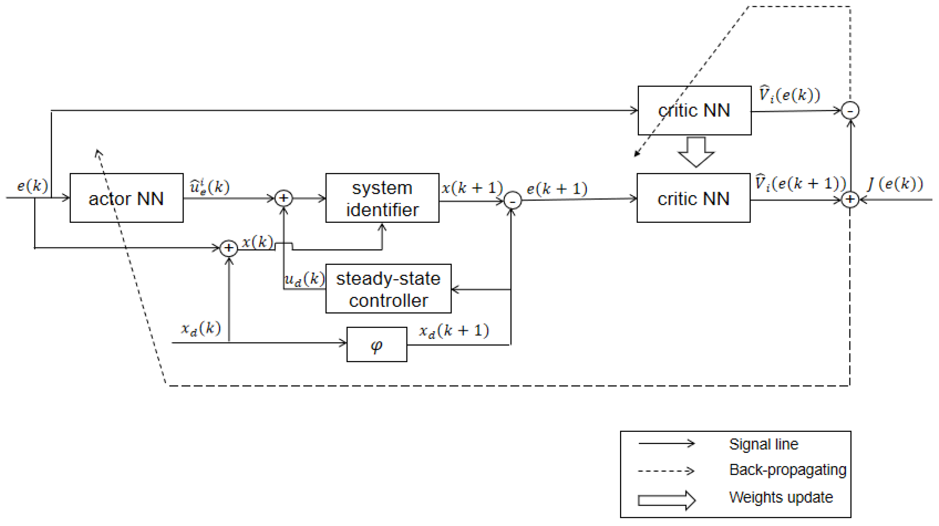
The working process of the proposed control technique is shown in
Figure 1. As shown in
Figure 1, with
,
and
, the estimated error
can be obtained by using the RBF-NN identifier and the steady-state controller. Corresponding to the steady-state controller
, we can obtain the reference trajectory
. Using the ADP algorithm, we can obtain nearly optimal feedback controller
. Then, the actual controller
and system dynamics
can be obtained. In addition, by using
and
the estimated tracking error
can be obtained,
can be further obtained. Finally, we can reconstruct the system dynamics to track the reference trajectory.
4. Simulation
In this section, we give the simulation results of our method and compare it with other methods [
36]. A discrete-time nonlinear system is introduced to demonstrate the effectiveness of the proposed tracking control method. The case is derived from [
24]. We assume that the nonlinear smooth function
is an unknown nonlinear drift function and
is a known function. The corresponding
and
are given as
The reference trajectory
for the above system is defined as
where
, and
of y-axis is chosen to have a
multiplied by
in the simulation.
4.1. Simulation Result of the Proposed Method
In this subsection, we give the simulation result for our proposed method.
Firstly, in order to deal with the unknown dynamics, we need to use two RBF networks to obtain the RBF identifier and the RBF steady-state controller. The RBF networks have a three-layer structure with two input neurons, hidden layers have nine neurons, and output layer have two neurons. The parameters
and
of the radial basis functions are chosen to be
and
, and the initial weights
are chosen to be random numbers between
. For the RBF identifier with its weights updating law (
21) to update the weights
, the unknown function
f is identified by the input/output data
. For the RBF steady-state controller, the reference trajectory data
and the weights updating law (
28) are used to update the weights
to identify the steady-state controller
. Because
, we can select
. According to
of Theorem 1, we can select
. For the control parameters
, because hidden layers have nine neurons,
,
, we select
. With control parameters
, we can know
and
from Theorem 1 and thus select
. The initial state is set as
. We trained the RBF networks with 10,000 steps of acquired data.
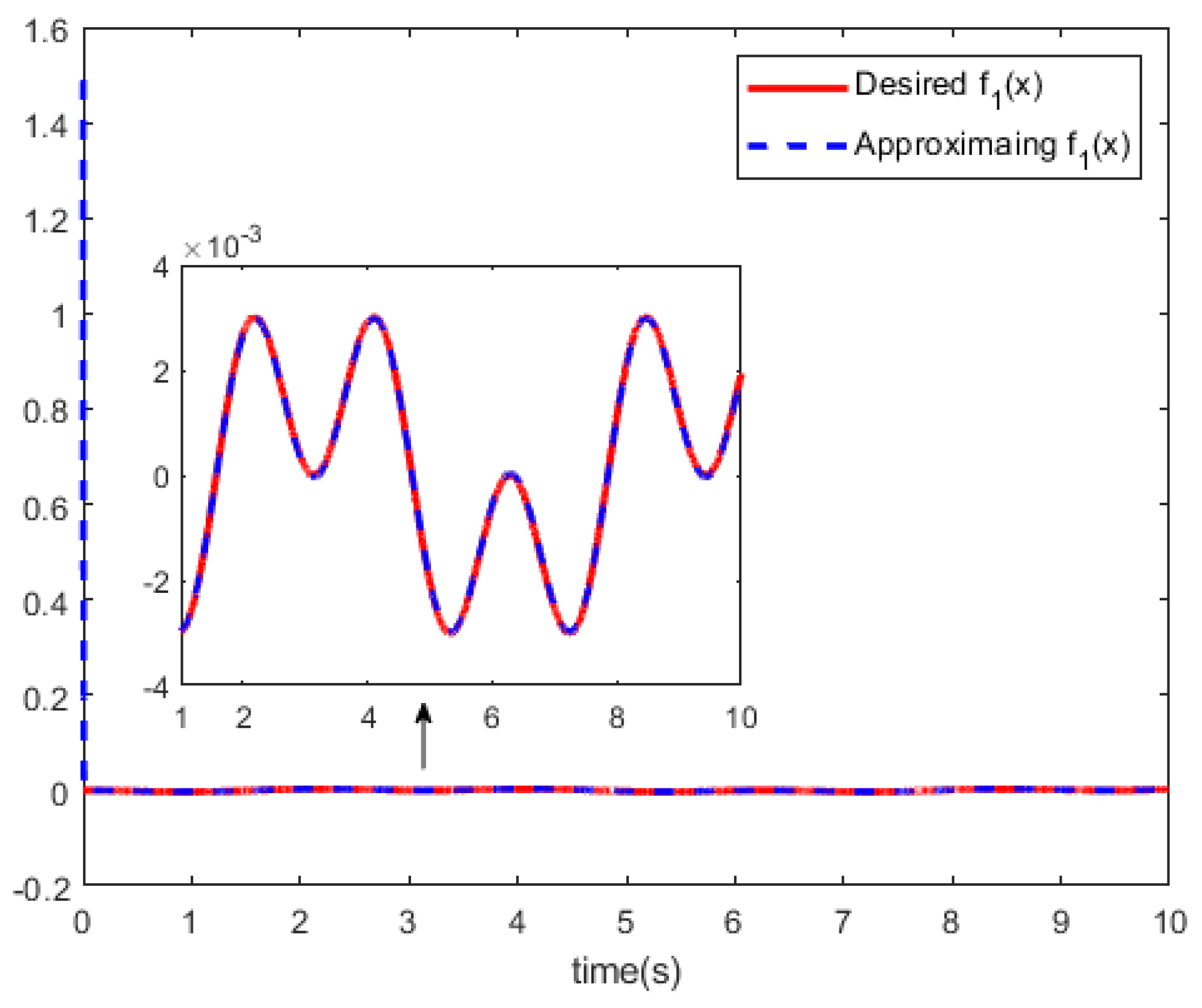
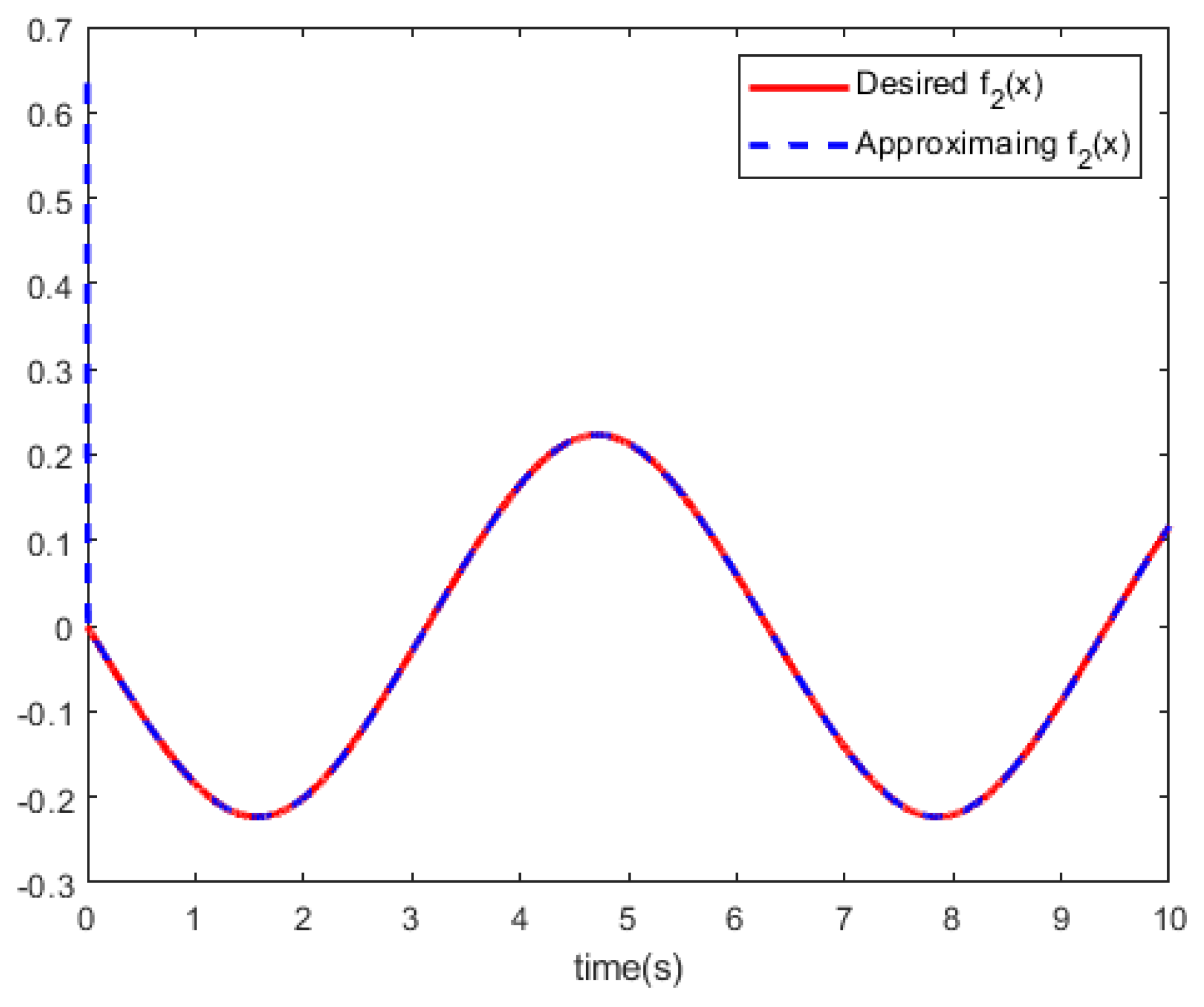
Figure 2 and
Figure 3 show the RBF-NN identifiers to approximate the tracking curves of the unknown dynamics
.
Then, based on the ADP algorithm of Bellman optimality, Equation (
6) was used to obtain the tracking error
e and the optimal feedback control
to train the critic network and the actor network, respectively. Meanwhile, the obtained standard control inputs
were used in system (
1), which keeps on looping until the value function
converge and the tracking error
is zero, where the performance index is selected as
and
, where
I is the identity matrix with appropriate dimension. For the actor network and the critic network, we used the same parameter settings. The initial weights of the critic networks and actor networks are randomly chosen between
. The input layer has 2 neurons, the hidden layer has 15 neurons, the output layer has 2 neurons, and the learning rate is 0.1. The hidden layer uses the function
and the function
, and the output layer uses the function
. Though parameter settings, we trained the actor network and the critic network with 5000 training steps to reach the given accuracy
.
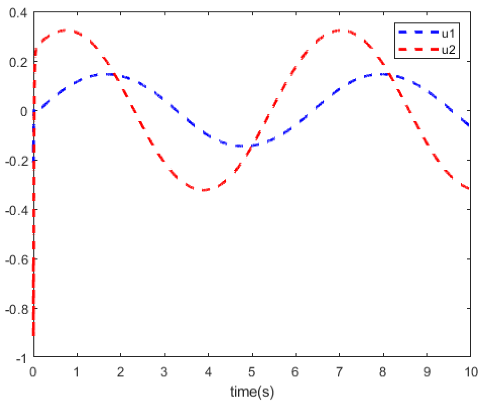
Figure 4 shows the curves of the system control
. In
Figure 5 and
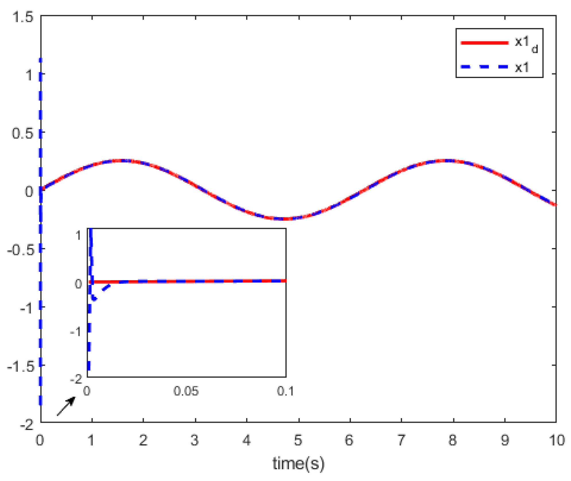
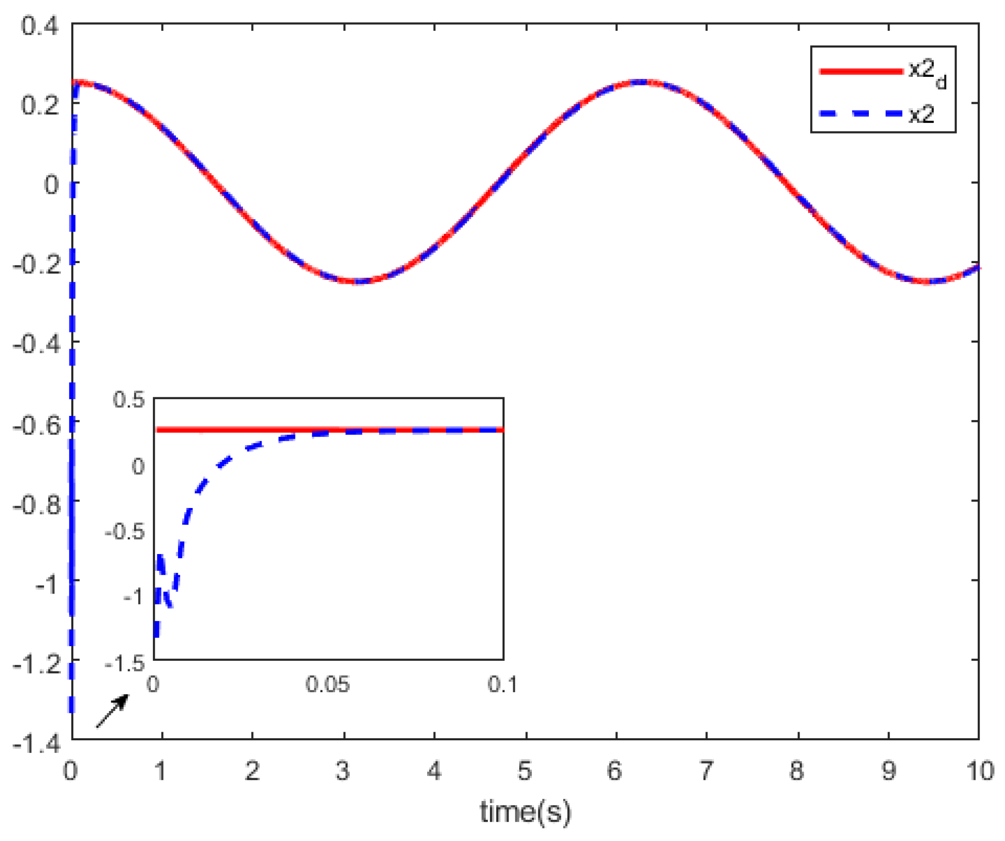
Figure 6, we can see the curves of the state trajectory
x and the reference trajectory
.
Based on above the results, the simulation results show that this tracking technique obtains a relatively satisfactory tracking performance for partially unknown discrete-time nonlinear systems.
4.2. Comparison with Other Methods
In this subsection, we will compare with the research results in [
36], which use a BP neural network to approximate the unknown system dynamics. In the comparison, we use the same system dynamics and desired tracking trajectory as (
61) and (
62) with the initial state
and the performance index
.
To begin with, an NN identifier is established by a three-layer BP neural network, which is chosen to have a 4–10–2 structure with four input neurons, eight hidden neurons, and two output neurons. The feedforward-neuro-controller is also established by a three-layer BP NN, which is chosen to have a 2–10–2 structure with two input neurons, eight hidden neurons, and two output neurons. For the NN identifier and the feedforward-neuro-controller, the parameter settings of the neural networks are identical, where the hidden layers use the sigmoidal function , the output layers use the linear function , the learning rate is 0.1, and the initial weights are chosen to be random numbers between .
For the actor network and the critic network, we also use the same parameter settings. A 2–15–2 structure is chosen for the critic networks and actor networks, the initial weights are randomly chosen between
, and the learning rate is 0.1. The hidden layer uses the function
and the function
, and the output layer uses the function
. Then, the given accuracy is
. In
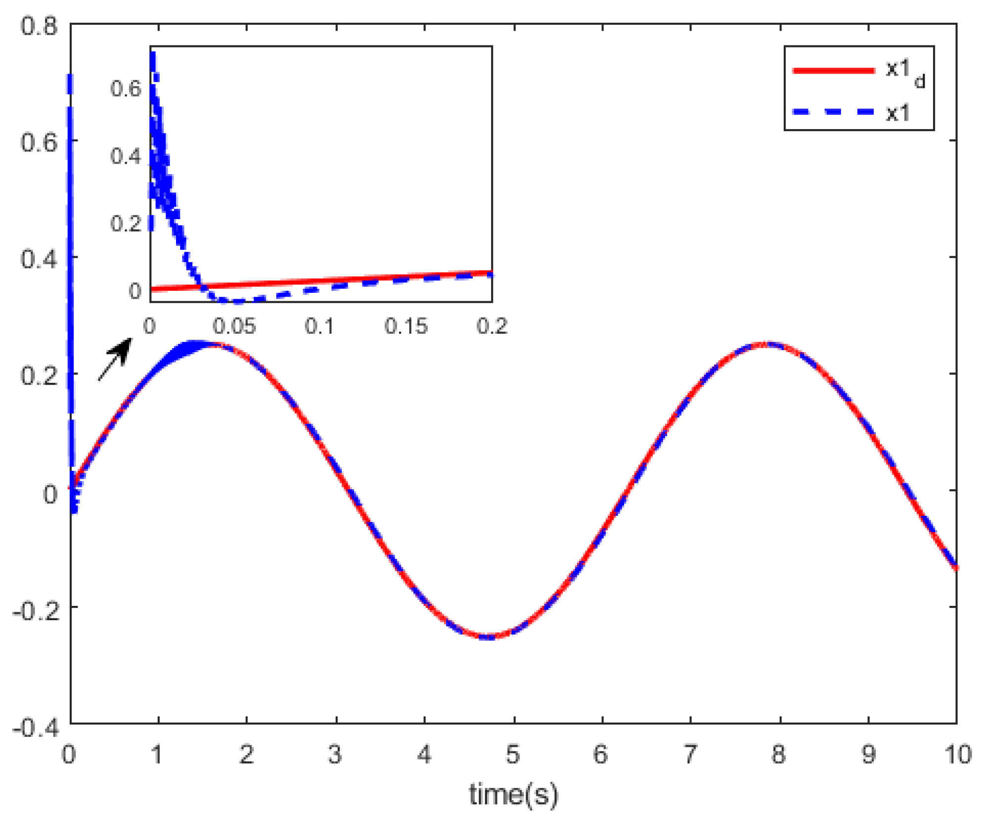
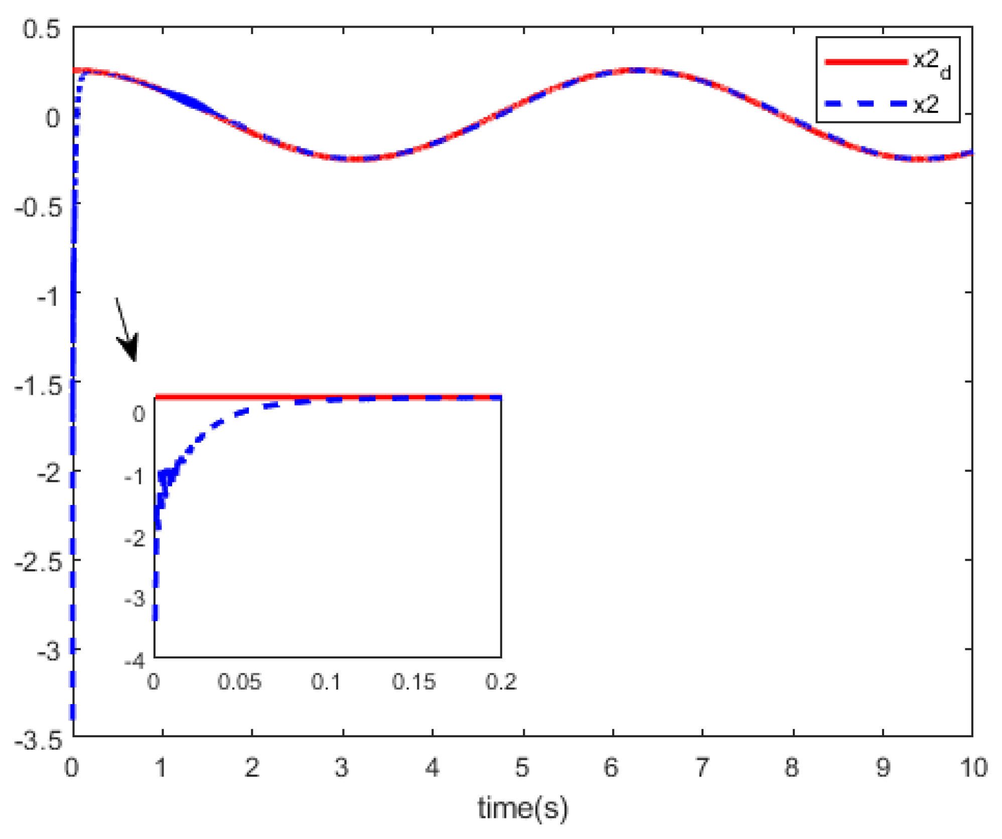
Figure 7 and
Figure 8, we can see the curves of the state trajectory
x and the reference trajectory
using tracking control methods for references.
Comparing the two methods, from
Figure 5,
Figure 6,
Figure 7 and
Figure 8, we can see that our method has better performance in tracking the reference trajectory.


