Abstract
Federated learning has become a prevalent distributed training paradigm, in which local devices collaboratively train learning models without exchanging local data. One of the most dominant frameworks of federated learning (FL) is FedAvg, since it is efficient and simple to implement; here, the first-order information is generally utilized to train the parameters of learning models. In practice, however, the gradient information may be unavailable or infeasible in some applications, such as federated black-box optimization problems. To solve the issue, we propose an innovative zeroth-order adaptive federated learning algorithm without using the gradient information, referred to as ZO-AdaFL, which integrates the zeroth-order optimization algorithm into the adaptive gradient method. Moreover, we also rigorously analyze the convergence behavior of ZO-AdaFL in a non-convex setting, i.e., where ZO-AdaFL achieves convergence to a region close to a stationary point at a speed of (T represents the total iteration number). Finally, to verify the performance of ZO-AdaFL, simulation experiments are performed using the MNIST and FMNIST datasets. Our experimental findings demonstrate that ZO-AdaFL outperforms other state-of-the-art zeroth-order FL approaches in terms of both effectiveness and efficiency.
Keywords:
black-box optimization; convergence rate; federated learning; gradient information; zeroth-order adaptive algorithm MSC:
68W40
1. Introduction
In the last few years, machine learning has received a lot of significant attention and enthusiasm. Deep learning especially has been successful in a range of applications, including ChatGPT, which is a notable example [1]. In deep learning, deep neural network models can be trained by using numerous data. Nevertheless, most of the data are generated and owned by personal devices like smartphones and PCs. The conventional method is to collect and transmit data to a central point, such as a data center. However, the data may leak the privacy of users during the process of transmission. Hence, it is difficult to train machine learning models by transmitting data from all users to the central server (CS), since the privacy and security of data need to be protected [2,3,4]. To mitigate this issue, FL is proposed in [5,6], where the raw data of the participating devices are kept locally; they participate in global machine learning model training in a collaborative manner by uploading local models instead of uploading data directly to the CS.
Because of its superiority, recently, a variety of optimization algorithms have been devoted to FL. One of the most popular FL approaches is the FedAvg algorithm [5]. Moreover, its variants have also been effectively discussed and understood recently [7,8,9]. Nonetheless, the aforementioned algorithms update the model parameters using stochastic gradient descent (SGD), which results in slow training and suboptimal performance. For this reason, adaptive gradient methods [10,11] were introduced in [12], which presents FedYogi and FedAdaGrad, respectively. Meanwhile, their convergence behaviors were also analyzed rigorously. Despite this progress, however, these algorithms need to have access to the gradient information during the training process. Nevertheless, this information might be unavailable in some real-world scenarios such as federated black-box optimization [13] and federated hyperparameter tuning [14]. Therefore, existing federated adaptive gradient methods are unsuitable for these scenarios.
One of the most popular gradient-free methods is the zeroth-order optimization algorithm, which has been successfully used in handling a variety of problems in the real world. The gradient information is expensive or infeasible, but the computation of objective functions is only available in these scenarios. Such examples include the black-box adversarial attack on structured prediction [15], reinforcement learning [16], and deep neural networks (DNNs) [17,18,19]. Due to its success, zeroth-order optimization has made great progress in recent years. Nesterov and Spokoiny [20] introduced a zeroth-order degree decrease (ZO-GD) algorithm by using a two-point Gaussian stochastic gradient estimator. Moreover, each gradient approximation requires only different function values. To improve the performance of zeroth-order optimization, a zeroth-order stochastic variance reduction algorithm known as ZO-SVRG was presented by Liu et al. [21]. Soon after, the ZO-AdaMM method was introduced in [22] as a zeroth-order adaptive momentum method for black-box optimization. The aim of this method is to reduce the large variance caused by the gradient estimator. Furthermore, an analysis of the convergence performance of ZO-AdaMM was also provided. The aforementioned efforts were made for the centralized machine learning framework. Nevertheless, the design and analysis of the zeroth-order optimization algorithm for the federated learning framework are still limited. Very recently, Fang et al. [23] presented the FedZO algorithm; several years ago, a federated zeroth-order optimization algorithm was presented, in which the zeroth-order gradient is integrated into federated learning. The SGD-based update rule is used in FedZO, which suffers from slow training speed. However, algorithmic and theoretical developments for federated adaptive zeroth-order optimization are still barely understood, to our knowledge.
Aspiring to remedy this gap in the research, this paper develops a communication efficient zeroth-order adaptive federated learning, referred to as ZO-AdaFL, under a non-convex setting. In each round of communication, ZO-AdaFL adopts the stochastic gradient estimator for multiple local model updates. Then, the adaptive gradient method is used to achieve a global update without first-order information. Meanwhile, multiple local iterations are implemented at each round of communication in ZO-AdaFL, which can reduce the communication overheads and is suitable in dealing with federated learning with numerous participants. Moreover, we also provide a theoretical guarantee for ZO-AdaFL for non-convex objective functions. This paper’s main contributions are summarized in the following points:
- We propose an algorithm for federated learning that aims to enhance communication efficiency, called zeroth-order adaptive federated learning (ZO-AdaFL), which inherits the framework of the FedAdam algorithm. Moreover, ZO-AdaFL only queries the values of objective functions without using gradient or Hessian information.
- We establish the convergence analysis of the proposed ZO-AdaFL algorithm under the non-convex setting. In particular, we prove that ZO-AdaFL achieves a convergence rate of with K local iterations and full device participation, where T represents the total number of iterations.
- We conduct various experiments to validate the performance of ZO-AdaFL. The experimental results show that ZO-AdaFL is effective and efficient compared with state-of-the-art federated zeroth-order learning methods.
The remaining work is organized as shown below. Section 2 introduces related work. We propose zeroth-order adaptive federated optimization in Section 3. In Section 4, we present the convergence analysis. We carefully verify our theoretical analysis through experiments in Section 5. We present the conclusion of this paper and discuss future work in Section 6. The notation interpretation is shown in Table 1.

Table 1.
Notation summary table.
Throughout this paper, we use and to denote the real number set and the expectation operator, respectively. Scalars, vectors, and matrices are denoted by regular letters, bold lower-case letters, and bold upper-case letters, respectively. The notation is used to represent a diagonal matrix with the diagonal entries determined by .
2. Related Work
In this section, we give a brief overview of related work on SGD, adaptive gradient methods, federated learning, zeroth-order optimization, respectively.
2.1. SGD and Adaptive Gradient Methods
SGD [24] is a popular method for training machine learning models, but it can be sensitive to parameter settings and slow to converge when dealing with heavy-tailed stochastic gradient noise. To address these issues, adaptive gradient methods like AdaGrad [25], RMSProp [26], and AdaDelta [27] can be used. Adam [10] and its variant AMSGrad [11] have been proposed. These methods are widely used in training deep neural networks and other variants [28,29,30] also have a crucial role in enhancing various aspects of the adaptive gradient method.
2.2. Federated Learning
FL is an innovative machine learning approach first mentioned by Google [5] in 2016 to address issues such as data privacy protection, security, and centralized processing bottlenecks. The technique allows data to be stored and models to be trained on local devices, but it also raises challenges in terms of communication efficiency, privacy protection, and device selection. To address these challenges effectively, FL [6] has now attracted considerable attention from the research community. Federated averaging (FedAvg) [5], as a classical framework, has strongly contributed to the rapid development of the field of FL through the periodic SGD updating of averages. Stich [31] provided a concise theoretical convergence guarantee for local SGD. Following the FedAvg algorithm, numerous other first-order optimization algorithms have been presented, e.g., FedProx [8], FedNova [7], and SCAFFOLD [32]. Furthermore, Reddi et al. [12] have also introduced a few adaptive federated optimization approaches in recent years, such as FedAdagrad, FedYogi, and FedAdam. These optimization approaches aim to yield even faster convergence to address the convergence problems of FedAvg. However, the mainstream first-order optimization algorithms have the following problems: the learning rate is too low, resulting in the too-slow convergence of the loss function; the learning rate is too high, which may affect the convergence and lead to fluctuations in the loss function on the minimum value, or even divergence, and is more sensitive to the parameters; the loss function is prone to converging to the local optimum, and it is difficult to jump out of the saddle point. To further reduce the communication overhead, several second-order optimization algorithms were proposed, such as GIANT [33], FedDANE [34], FedNL [35], and FedNew [36]. The second-order optimization algorithm accelerates the first-order gradient descent by using the curvature correction of the second-order derivative of the objective function. Compared to the first-order optimizer, it converges faster, highly approximates the optimal value, and the descent path is geometrically more consistent with the true optimal descent path. Although first-order and second-order optimization algorithms have made significant contributions to federated learning, they may not be suitable for scenarios where derivative or Hessian information is unavailable or large-scale datasets need to be trained. In such cases, zeroth-order optimization algorithms can be more effective. Zeroth-order optimization algorithms are advantageous due to their computational efficiency, independence from the gradient problem, and ability to adapt to non-smooth and discrete objective functions. Therefore, using zeroth-order optimization algorithms in these situations can be more efficient and effective.
2.3. Zeroth-Order Optimization
The ZO algorithm commonly uses a gradient estimator, such as the one-point or two-point gradient estimator, to approximate the full-gradient. The one-point gradient estimator estimates the gradient by evaluating the function at a random nearby location to the point [37,38]. On the other hand, the two-point gradient estimator uses two stochastic function queries to compute the finite difference [20,39]. ZO stochastic gradient descent (ZO-SGD) [40] and ZO stochastic coordinate descent (ZO-SCD) [41] are able to converge quickly in unconstrained stochastic optimization problems with a convergence rate of ; the number of optimization variables is d with T iterations. To enhance the iteration complexity of ZO algorithms, the variance reduction technique has been applied to ZO-SGD and ZO-SCD, resulting in stochastic-variation-reduced ZO algorithms, with an enhanced convergence rate in T, i.e., [21,42,43]. Several recent works [13,44] have concentrated on the study of distributed zeroth-order optimization. In particular, the authors of [44] have developed a ZONE algorithm using the primal–dual technique. However, ZONE requires sampling complexity per iteration. More comprehensive discussion on distributed zeroth-order optimization methods can be found in [45,46].
3. Zeroth-Order Adaptive Federated Optimization
Most federated optimization algorithms that utilize SGD to update the model have loss function values that are slow to change in some dimensions. They tend to fall into local minima and at saddle points in high-dimensional spaces, which leads to larger variance values of the loss function and hinders the algorithm’s convergence speed. In this paper, we devote much attention to two-point gradient estimators that aim to make the variance of the loss function smaller, thus speeding up the convergence of the algorithm and improving the complexity bounds of the ZO algorithms. Firstly, we analyze the non-convex optimization problems of FL; secondly, we propose an FL optimization algorithm called ZO-AdaFL. An overview flowchart of the ZO-AdaFL algorithm is shown in Figure 1.
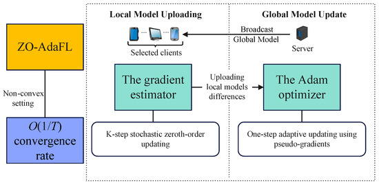
Figure 1.
The ZO-AadFL algorithm overview flowchart.
3.1. Problem Formulation
In FL, general FL algorithms have difficulty solving complex optimization models without gradients or where obtaining gradients is costly. This scenario occurs in many real-world applications, including—but not limited to—federal black-box attacks on DNNs [13]. The objective function in FL is typically non-convex due to the heterogeneity of client data. Furthermore, the problem of federated black-box attacks on DNN models is non-convex. Meanwhile, considering the practical application scenario of large-scale device participation and black-box attacks in FL, this paper aims to study the non-convex optimization problem in FL; the specific problem is described here:
where m is the total number of clients, represents the model parameter with dimension d, and represents the global loss function on the CS. In Equation (1), is a local non-convex loss function and is a measure of the expectation of risk above locally distributed data, denoted by where represents a random variable, , uniformly sampled from ; denotes the loss relative to which is evaluated at the model parameter .
In the FedAvg, an optimization solution is proposed for the problem involved in problem Equation (1). During the t-th iteration, the CS provides client i in the chosen subset with the model . Using the learning rate , the client i performs the K steps of the SGD update locally to obtain the local model . Each client can perform model updates based on local data and send the model parameter differences back to the CS. Then, the differences in the global model, denoted as , are updated by the CS through the simple averaging of the local model differences, . The global model is updated using the function , which is the same approach as that taken for the direct average local model , i.e., .
FedAdam was then proposed among several adaptive optimization methods in federated learning [12]. FedAdam replaces FedAvg’s SGD approach by introducing the Adam optimizer as a global update rule that can better accommodate different local variances and average them out to . The CS then uses the Adam optimizer to perform an accurate and fast update of the global model based on this global variance :
where serves as a pseudo gradient, and the global update can be considered as a single-step Adam update that uses . There have also been a number of algorithm variants proposed that make subtle modifications to the variance term , including FedAdagrad [12], FedYogi [12] and FedAMSGrad [47]. In order to prevent the term from becoming too small and causing instability in the optimization process, stability is ensured by adding to Equation (4).
3.2. ZO-AdaFL Algorithm
As shown in Algorithm 1, this section proposes a general zeroth-order algorithm for an adaptive federated optimization framework. The ZO-AdaFL algorithm aims to eliminate gradient dependence and focuses on reducing the model exchange frequency. To achieve these goals, in each round of communication, the ZO-AdaFL algorithm cleverly employs a gradient estimator and performs a K-step stochastic zeroth-order updating strategy. Each round of our ZO-AdaFL algorithm has the following four parts.
Broadcast Global Model: The CS chooses any collection of clients from the M clients for training at the beginning of round t, denoted as . Subsequently, each client in collection obtains a current global model parameter in a broadcast from the CS.
Local Model Update: Each selected client, , then trains its own local model parameters, , using K-steps of stochastic zeroth-order updating at a learning rate of . Specifically, at the k-th iteration of the t-th round, client i computes a two-point stochastic gradient estimator [45], as shown below.
where denotes the local model of client i, and is a personalized update of client i in each iteration. Specifically, is a random variable obtained by sampling a local data distribution of client i at the k-th iteration of the t-th round. is a random direction vector obtained by evenly sampling on the unit sphere of dimension d. denotes the magnitude of the movement in that random direction, i.e., the positive step size.
Afterwards, client i performs a stochastic zeroth-order update to update its local model, as follows:
where represents the learning rate. Client i obtains a new local model parameter through a total of k iterations.
Local Model Uploading: After the local training is completed, all of the clients from obtain the updated part of the local model parameters, i.e., . Then, they upload them to the CS.
Global Model Update: The CS aggregates to obtain after it receives the local model update from the selected client i, i.e., . acts as a pseudo gradient to calculate momentum and variance , following Equations (2) and (3). Subsequently, the CS obtains the new global model, that is, , where . Note that this is the same as the AMSGrad update rule [11], which addresses Adam’s non-convergence problem [10] by using non-decreasing .
| Algorithm 1 Zeroth-Order Adaptive Optimization for Federated Learning (ZO-AdaFL) |
Require: initial model , local step size , global step size , smoothing parameter , .
|
4. Convergence Analysis
The presentation in this section is about the theoretical convergence results of ZO-AdaFL. We focus on the setting of non-convex loss functions. In order to perform the convergence analysis, we need some assumptions. These assumptions are presented below.
Assumption 1
(Smoothness). Each loss function on the i-th worker is L-smooth, i.e., ,
Assumption 1 also implies the L-gradient Lipschitz condition, i.e., . Assumption 1 is a standard assumption in non-convex optimization problems, which has been also adopted in [10,11,48,49].
Assumption 2
(Bounded Gradient). Each loss function on the i-th worker has bounded stochastic gradient on , i.e., for all ξ, we have .
The assumption of bounded gradient is usually adopted in adaptive gradient methods [10,11,28,50].
Assumption 3
(Unbiasedness). The stochastic gradient is an unbiased estimate of , i.e.,
Assumption 4
(Bounded Variance). Each stochastic gradient on the i-th worker has a bounded local variance, i.e., for all , we have , and the loss function on each worker has a global variance bound, , where and represent the local stochastic gradient variance and global variance, respectively.
Assumption 4 is commonly applied in FL optimization issues [12,48,49]. The bounded local variance reflects the stochastic gradient stochasticity for each client, and the bounded global variance reflects the heterogeneity of the dataset across devices. When the value of the local variance is 0 (i.e., ), it represents a setting where the dataset for each client has the same distribution, i.e., independent and identically distributed (i.i.d.).
Here, we show the convergence results of ZO-AdaFL using an all-hands-on-deck scheme, where each client participates in the communication round and the model update, denoted as . Before proving the convergence results of ZO-AdaFL, several auxiliary lemmas are introduced.
Lemma 1.
Under Assumption 1, using the ZO-AdaMM update rule [22], we have
Proof.
See Appendix A. □
Lemma 2.
Suppose Assumptions 1–4 hold. Then, according to the ZO-AdaMM update rule [22], for the first term of Lemma 1, we have
Proof.
See Appendix B. □
Lemma 3.
Then, with Assumptions 1–4 and , for the second term of Lemma 1, we have
Proof.
The proof follows from Lemma 2.4 in [22]. □
Theorem 1.
Suppose Assumptions 1–4 hold. If the local learning rate satisfies , then, under the condition of the full participation of the devices, the iterates of ZO-AdaFL in Algorithm 1 satisfy
where , , and . Moreover, as the communication rounds increase, ZO-AdaFL converges to the neighborhood of a solution.
Proof of Theorem 1.
See Appendix C. □
Remark 1.
Equation (10) shows that the upper bound of the minimum gradient squared in the global model sequence is closely related to the total number of steps T, and it decreases as . Additionally, the convergence rate of the algorithm depends on and . In the scenario where each worker has the same data distribution (i.e., i.i.d.), the global variance is zero (), and the variance term Ψ will be reduced, relying less on the number of local steps K.
Remark 2.
Note that, compared with FedAdam [12], our theoretical analysis of ZO-AdaFL improves upon previous work by providing a comprehensive analysis of ZO-AdaFL with a non-zero momentum term. In contrast, the analysis in reference [12] only focuses on the scenario where .
5. Simulation Results
In this section, we introduce the results of our simulated experiments, evaluating the performance of the ZO-AadFL algorithm, which is proposed for federated black-box attacks. We verify the effectiveness of our ZO-AadFL under federated black-box attacks and the faster convergence speed of ZO-AadFL with the involvement of large-scale devices through different experimental setups.
5.1. Federated Black-Box Attack
Deep-learning-based image classification algorithms are mostly trained under carefully made datasets. For images outside the dataset or slightly modified images, the recognition ability of the network is often affected to some extent. Under this phenomenon, adversarial attacks begin to be included in the examination of network model robustness. By adding different noises or transforming certain areas of the image to generate antagonistic samples, the samples attack the network model to achieve the purpose of confusing the network. Since the black-box possesses the characteristic of not being able to directly observe the gradient information of the function, we need to solve the black-box attack optimization problem with zeroth-order optimization. We consider a well-trained DNN classifier model with a testing accuracy of on the standard MNIST dataset [13], and let this model simulate a federated black-box model. The federated black-box attack aims to jointly produce a universal adversarial perturbation that makes the perturbation image visually imperceptible, but this can mislead the classifier.
5.2. Experiment Setup
In this experiment setting, we randomly selected 200 samples from the training set of digit class “4”, and then distributed samples to each client i. The number of clients was set to . Moreover, and , , , . The learning rate and step size were set to and , respectively.
5.3. Experimental Results and Analysis
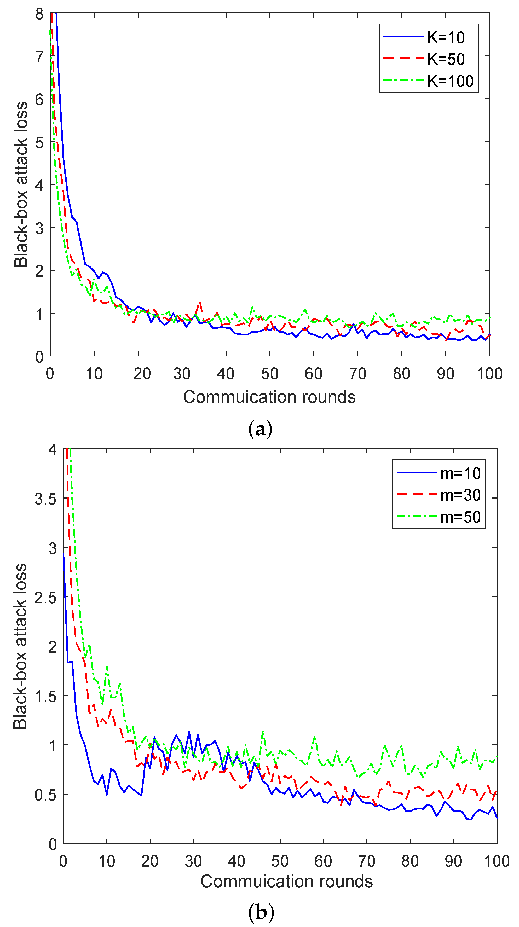
In the experiment, we observed the influence of a different number of local iterations and the number of participating clients on the convergence of ZO-AdaFL algorithm. The results are shown in Figure 2.
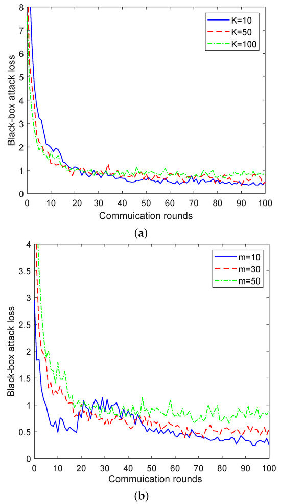
Figure 2.
Black-box attack loss for the ZO-AadFL algorithm vs. communication rounds. (a) Influence of number of local iterations. (b) Influence of number of participating clients.
In Figure 2a, we demonstrate the effect that the number of local iterations has on the convergence performance of ZO-AadFL when the total number of clients involved . Specifically, the relationship between the black-box attack loss and the number of communication rounds is presented by changing the number of local iterations . As shown in Figure 2a, as K increases, the attack loss of the ZO-AadFL algorithm decreases and the convergence rate tends to accelerate. It is worth noting that the ZO-AadFL algorithm converges to different losses for different K; this is because, with the non-convex nature of the federated black-box attack problem on DNN models, multiple saddle points exist. As a result, the ZO-AadFL algorithm may become trapped in any of these saddle points. In addition, Figure 2b shows the black-box attack losses of ZO-AadFL for different numbers of participating clients when the number of local iterations is . Specifically, the relationship between attack losses and communication rounds is presented by changing the number of participating clients . It can be observed that the ZO-AadFL is able to effectively reduce attack losses and produce a better convergence effect with the increase in m, because the more clients participate in training, the higher the precision of model training.
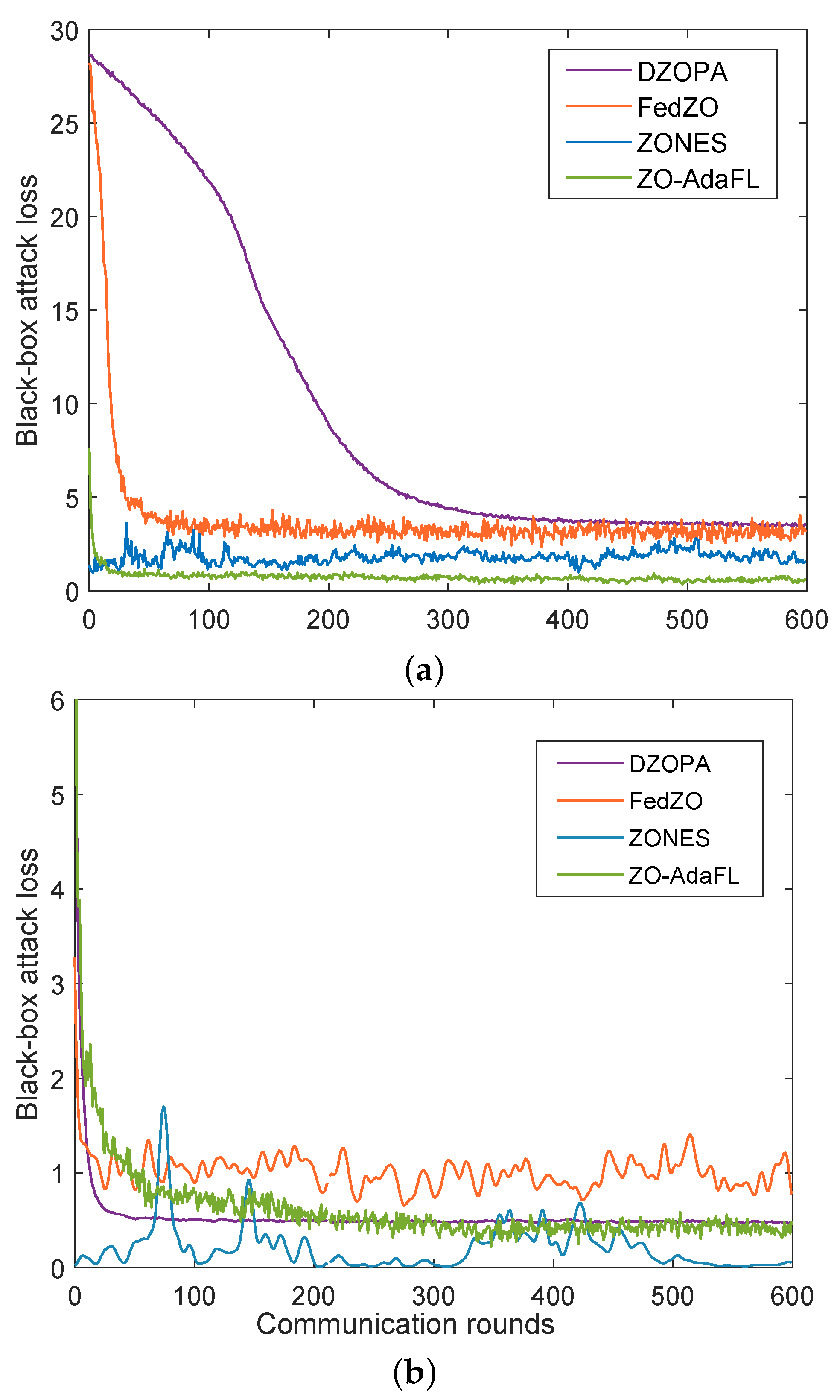
We further verified the effectiveness of the proposed ZO-AdaFL algorithm, and compared the performance of our algorithm with those of three baseline algorithms—i.e., the DZOPA [13], FedZO [23], and ZONES [44] algorithms—on training MNIST and FMNIST datasets, respectively, with the CNN model. The results are depicted in Figure 3. We compared communication rounds and the black-box attack loss for several algorithms on each dataset.
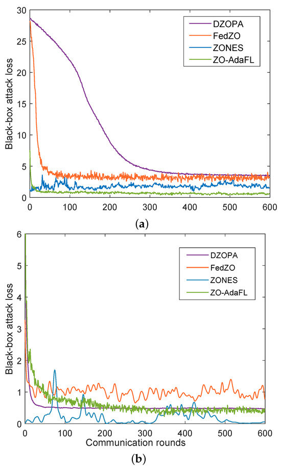
Figure 3.
Test training loss for different algorithms on MNIST and FMNIST datasets. (a) Training loss for different algorithms on MNIST dataset. (b) Training loss for different algorithms on FMNIST dataset.
For the MNIST experiments, Figure 3a shows the convergence result of ZO-AdaFL and other ZO optimization baselines. In the initial stage, the attack loss of each algorithm is high. As the number of communication rounds increases, the attack loss of all algorithms gradually decreases. Furthermore, our ZO-AdaFL algorithm’s loss decreases at a faster rate and ultimately reaches the lowest loss value. Note that—although DZOPA and FedZO have similar final performances—the DZOPA algorithm does not perform as well as FedZO when the number of communication rounds is low. Throughout the experiment, although the attack loss of the ZONES algorithm is always kept at a relatively lower level than that of FedZO, it is more volatile and less stable. Compared with the FedZO algorithm, the ZO-AadFL algorithm reduces the attack loss faster and has better convergence in the first 100 rounds. Based on the comparative analysis of the experimental results of the FedZO algorithm and the ZO-AadFL algorithm, we find that the loss of the ZO-AadFL algorithm is smaller than that of the FedZO algorithm, both in the initial and final stages. In contrast, ZO-AadFL significantly outperforms the other three baselines in terms of final black-box attack loss. This suggests that ZO-AadFL can be an ideal solution for zeroth-order optimization algorithms in the absence of first-order information.
For FMNIST experiments, Figure 3b shows the convergence result of ZO-AdaFL and other ZO optimization baselines. Obviously, our ZO-AadFL algorithm converges with the number of algorithmic communication rounds grown. Furthermore, the final black-box attack loss performance of ZO-AadFL algorithm is better than FedZO and DZOPA algorithms. However, compared to the ZONES algorithm, our algorithm has a higher attack loss rate. To further analyze the reasons for this phenomenon, we provide additional experimental results about the attack success rate and the distortion loss against 600 communication rounds in Table 2. It is important to note that all algorithms start with no perturbation. Consequently, the attack loss gradually decreases with the number of algorithmic communication rounds, which grows till it converges to zero, demonstrating a successful attack. Meanwhile, there is a possibility of an increase in distortion loss. In these circumstances, if the algorithm can quickly converge to where the optimal trade-off between zero attack loss and low distortion loss is reached, then the algorithm achieves optimal attack performance. In other words, there exists a trade-off between attack loss and perturbation distortion. Combining Figure 3b and Table 2, the ZONES algorithm achieves better attack loss performance due to its higher disturbance loss compared to our proposed algorithm. However, the success rate of our proposed algorithm in attacking is higher. Moreover, our proposed algorithm sacrifices disturbance loss to achieve lower attack loss and higher attack success rate, compared to the DZOPA and FedZO algorithms.
Table 2.
Summary of attack success rate and distortion loss for universal attack against under iterations on the FMNIST dataset.
6. Conclusions and Future Work
In this paper, we propose a zeroth-order adaptive optimization algorithm for FL, named ZO-AdaFL, which is the first application of zeroth-order optimization and adaptive optimization to FL. ZO-AdaFL adopts the zero-order optimization algorithm of estimating the gradient by function values to approximate the gradient to solve the FL black-box optimization problem, and the adaptive algorithm avoids FL falling into a local optimum under the non-convex setup condition of full device participation. The convergence speed of the ZO-AdaFL algorithm is also guaranteed. We also analyze the convergence behavior of the ZO-AdaFL algorithm theoretically and prove its convergence rate, , in a non-convex setting. The experiments conducted on a variety of benchmarks confirmed our theoretical analysis. In this work, we assume that evaluation on can be made in the absence of noise or error, which may limit the applicability of this result, since—in many practical scenarios—the functional values are obtained through some noisy measurement procedures. Because the variance of the stochastic gradient estimator can be unbounded, in the future, we hope to further incorporate the idea of variance reduction to minimize the constraints. Meanwhile, a distributed zero-order algorithm can be investigated on this basis.
Author Contributions
Conceptualization, P.X.; methodology, P.X.; software, P.X. and X.G.; validation, X.G., F.L., Y.Z. and H.S.; formal analysis, F.L.; investigation, P.X. and L.X.; resources, F.L.; data curation, P.X. and X.G.; writing—original draft preparation, P.X. and X.G.; writing—review and editing, X.G., F.L. and Y.Z.; supervision, Y.Z.; project administration, H.S.; funding acquisition, P.X. and L.X. All authors have read and agreed to the published version of the manuscript.
Funding
This research was funded by the National Natural Science Foundation of China (NSFC) under Grants No. 61801171 and 62072158, in part by the Henan Province Science Fund for Distinguished Young Scholars (222300420006), and Program for Innovative Research Team in University of Henan Province (21IRTSTHN015).
Data Availability Statement
In this study, we used publicly available datasets—FMNIST and MNIST. The model files used for the comparison experiments can be acquired from the respective authors.
Conflicts of Interest
The authors declare no conflicts of interest.
Abbreviations
The following abbreviations are used in this manuscript:
| FL | federated learning |
| ZO-AdaFL | zeroth-order adaptive federated learning |
| CS | central server |
| SGD | stochastic gradient descent |
| DNNs | deep neural networks |
| ZO-GD | zeroth-order degree decrease |
| ZO-SGD | zeroth-order stochastic gradient descent |
| ZO-SCD | zeroth-order stochastic coordinate descent |
Appendix A
Proof.
Before we can prove it, we need to introduce a sequence auxiliary variable, , which is very common in adaptive methods.
According to the smoothness of function f, we can obtain
Suppose and , we have
and thus
We further obtain
Summing t from 1 to T and take expectation, we can obtain
The proof is now complete. □
Appendix B
Proof.
Here, we recall the notation diag diag(max.
where the first inequality follows by the fact that . For the first term in Equation (A10), we can obtain Equation (A11).
We further analyze the last item in Equation (A11). According to the properties of the gradient estimator ([51] Lemma 4.2), . Thus, we can obtain Equation (A12), where the third equality follows from , the first inequality holds by applying Cauchy–Schwarz inequality; the second inequality follows from Assumption 1.
According to ([23], Lemma 2), when , we have
For the second term in Equation (A10), we have
where the last inequality from ([52], Lemma C.1). Since f has -bounded stochastic gradients, for any and , we have .
Now, let us analyze
Thus, we have Equation (A18).
At this point, the proof has been completed. □
Appendix C
Proof of Theorem 1.
By combining Lemmas 1, 2, and 3, we can obtain
By submitting ([52], Lemma C.2, Lemma C.5) into Equation (A19), and using the fact that , we have Equation (A20). The last inequality holds due to additional constraint of local learning rate with the inequality , we have the constraint .
Then, we can obtain
Therefore,
where , , and . □
References
- Abdullah, M.; Madain, A.; Jararweh, Y. ChatGPT: Fundamentals, Applications and Social Impacts. In Proceedings of the 9th International Conference on Social Networks Analysis, Management and Security, SNAMS 2022, Milan, Italy, 29 November–1 December 2022; pp. 1–8. [Google Scholar] [CrossRef]
- Shen, S.; Zhu, T.; Wu, D.; Wang, W.; Zhou, W. From distributed machine learning to federated learning: In the view of data privacy and security. Concurr. Comput. Pract. Exp. 2022, 34, e6002. [Google Scholar] [CrossRef]
- Guo, X. Federated Learning for Data Security and Privacy Protection. In Proceedings of the 12th International Symposium on Parallel Architectures, Algorithms and Programming, PAAP 2021, Xi’an, China, 10–12 December 2021; pp. 194–197. [Google Scholar] [CrossRef]
- Yu, S.; Cui, L. Introduction to Federated Learning. In Security and Privacy in Federated Learning; Springer Nature: Singapore, 2023; pp. 1–11. [Google Scholar] [CrossRef]
- McMahan, B.; Moore, E.; Ramage, D.; Hampson, S.; y Arcas, B.A. Communication-Efficient Learning of Deep Networks from Decentralized Data. In Proceedings of the 20th International Conference on Artificial Intelligence and Statistics, AISTATS 2017, Fort Lauderdale, FL, USA, 20–22 April 2017; Volume 54, pp. 1273–1282. [Google Scholar]
- Konečný, J.; McMahan, H.B.; Yu, F.X.; Richtárik, P.; Suresh, A.T.; Bacon, D. Federated Learning: Strategies for Improving Communication Efficiency. arXiv 2016, arXiv:1610.05492. [Google Scholar]
- Wang, J.; Liu, Q.; Liang, H.; Joshi, G.; Poor, H.V. A Novel Framework for the Analysis and Design of Heterogeneous Federated Learning. IEEE Trans. Signal Process. 2021, 69, 5234–5249. [Google Scholar] [CrossRef]
- Li, T.; Sahu, A.K.; Zaheer, M.; Sanjabi, M.; Talwalkar, A.; Smith, V. Federated Optimization in Heterogeneous Networks. In Proceedings of the Machine Learning and Systems 2020, MLSys 2020, Austin, TX, USA, 2–4 March 2020. [Google Scholar]
- Zhang, X.; Hong, M.; Dhople, S.V.; Yin, W.; Liu, Y. FedPD: A Federated Learning Framework With Adaptivity to Non-IID Data. IEEE Trans. Signal Process. 2021, 69, 6055–6070. [Google Scholar] [CrossRef]
- Kingma, D.P.; Ba, J. Adam: A Method for Stochastic Optimization. In Proceedings of the 3rd International Conference on Learning Representations, ICLR 2015, San Diego, CA, USA, 7–9 May 2015. [Google Scholar]
- Reddi, S.J.; Kale, S.; Kumar, S. On the Convergence of Adam and Beyond. In Proceedings of the 6th International Conference on Learning Representations, ICLR 2018, Vancouver, BC, Canada, 30 April–3 May 2018. [Google Scholar]
- Reddi, S.J.; Charles, Z.; Zaheer, M.; Garrett, Z.; Rush, K.; Konečný, J.; Kumar, S.; McMahan, H.B. Adaptive Federated Optimization. In Proceedings of the 9th International Conference on Learning Representations, ICLR 2021, Virtual, 3–7 May 2021. [Google Scholar]
- Yi, X.; Zhang, S.; Yang, T.; Johansson, K.H. Zeroth-order algorithms for stochastic distributed non-convex optimization. Automatica 2022, 142, 110353. [Google Scholar] [CrossRef]
- Dai, Z.; Low, B.K.H.; Jaillet, P. Federated Bayesian Optimization via Thompson Sampling. In Proceedings of the Advances in Neural Information Processing Systems 33: Annual Conference on Neural Information Processing Systems 2020, NeurIPS 2020, Virtual, 6–12 December 2020. [Google Scholar]
- Taskar, B.; Chatalbashev, V.; Koller, D.; Guestrin, C. Learning structured prediction models: A large margin approach. In Proceedings of the Machine Learning, Proceedings of the Twenty-Second International Conference (ICML 2005), Bonn, Germany, 7–11 August 2005; Volume 119, pp. 896–903. [Google Scholar] [CrossRef]
- Choromanski, K.; Rowland, M.; Sindhwani, V.; Turner, R.E.; Weller, A. Structured Evolution with Compact Architectures for Scalable Policy Optimization. In Proceedings of the 35th International Conference on Machine Learning, ICML 2018, Stockholmsmässan, Stockholm, Sweden, 10–15 July 2018; Volume 80, pp. 969–977. [Google Scholar]
- Papernot, N.; McDaniel, P.D.; Goodfellow, I.J.; Jha, S.; Celik, Z.B.; Swami, A. Practical Black-Box Attacks against Machine Learning. In Proceedings of the 2017 ACM on Asia Conference on Computer and Communications Security, AsiaCCS 2017, Abu Dhabi, United Arab Emirates, 2–6 April 2017; pp. 506–519. [Google Scholar] [CrossRef]
- Chen, P.; Zhang, H.; Sharma, Y.; Yi, J.; Hsieh, C. ZOO: Zeroth Order Optimization Based Black-box Attacks to Deep Neural Networks without Training Substitute Models. In Proceedings of the 10th ACM Workshop on Artificial Intelligence and Security, AISec@CCS 2017, Dallas, TX, USA, 3 November 2017; pp. 15–26. [Google Scholar] [CrossRef]
- Kurakin, A.; Goodfellow, I.J.; Bengio, S. Adversarial Machine Learning at Scale. In Proceedings of the 5th International Conference on Learning Representations, ICLR 2017, Toulon, France, 24–26 April 2017. [Google Scholar]
- Nesterov, Y.E.; Spokoiny, V.G. Random Gradient-Free Minimization of Convex Functions. Found. Comput. Math. 2017, 17, 527–566. [Google Scholar] [CrossRef]
- Liu, S.; Kailkhura, B.; Chen, P.; Ting, P.; Chang, S.; Amini, L. Zeroth-Order Stochastic Variance Reduction for non-convex Optimization. In Proceedings of the Advances in Neural Information Processing Systems 31: Annual Conference on Neural Information Processing Systems 2018, NeurIPS 2018, Montréal, QC, Canada, 3–8 December 2018; pp. 3731–3741. [Google Scholar]
- Chen, X.; Liu, S.; Xu, K.; Li, X.; Lin, X.; Hong, M.; Cox, D.D. ZO-AdaMM: Zeroth-Order Adaptive Momentum Method for Black-Box Optimization. In Proceedings of the Advances in Neural Information Processing Systems 32: Annual Conference on Neural Information Processing Systems 2019, NeurIPS 2019, Vancouver, BC, Canada, 8–14 December 2019; pp. 7202–7213. [Google Scholar]
- Fang, W.; Yu, Z.; Jiang, Y.; Shi, Y.; Jones, C.N.; Zhou, Y. Communication-Efficient Stochastic Zeroth-Order Optimization for Federated Learning. IEEE Trans. Signal Process. 2022, 70, 5058–5073. [Google Scholar] [CrossRef]
- Sinha, N.K.; Griscik, M.P. A Stochastic Approximation Method. IEEE Trans. Syst. Man Cybern. 1971, 1, 338–344. [Google Scholar] [CrossRef]
- Duchi, J.C.; Hazan, E.; Singer, Y. Adaptive Subgradient Methods for Online Learning and Stochastic Optimization. J. Mach. Learn. Res. 2011, 12, 2121–2159. [Google Scholar]
- Tieleman, T.; Hinton, G. Lecture 6.5-rmsprop: Divide the gradient by a running average of its recent magnitude. COURSERA Neural Netw. Mach. Learn. 2012, 4, 26–31. [Google Scholar]
- Zeiler, M.D. ADADELTA: An Adaptive Learning Rate Method. arXiv 2012, arXiv:1212.5701. [Google Scholar]
- Chen, J.; Zhou, D.; Tang, Y.; Yang, Z.; Cao, Y.; Gu, Q. Closing the Generalization Gap of Adaptive Gradient Methods in Training Deep Neural Networks. In Proceedings of the Twenty-Ninth International Joint Conference on Artificial Intelligence, IJCAI 2020, Yokohama, Japan, 11–17 July 2020; pp. 3267–3275. [Google Scholar] [CrossRef]
- Luo, L.; Xiong, Y.; Liu, Y.; Sun, X. Adaptive Gradient Methods with Dynamic Bound of Learning Rate. In Proceedings of the 7th International Conference on Learning Representations, ICLR 2019, New Orleans, LA, USA, 6–9 May 2019. [Google Scholar]
- Loshchilov, I.; Hutter, F. Decoupled Weight Decay Regularization. In Proceedings of the 7th International Conference on Learning Representations, ICLR 2019, New Orleans, LA, USA, 6–9 May 2019. [Google Scholar]
- Stich, S.U. Local SGD Converges Fast and Communicates Little. In Proceedings of the 7th International Conference on Learning Representations, ICLR 2019, New Orleans, LA, USA, 6–9 May 2019. [Google Scholar]
- Karimireddy, S.P.; Kale, S.; Mohri, M.; Reddi, S.J.; Stich, S.U.; Suresh, A.T. SCAFFOLD: Stochastic Controlled Averaging for Federated Learning. In Proceedings of the 37th International Conference on Machine Learning, ICML 2020, Virtual, 13–18 July 2020; Volume 119, pp. 5132–5143. [Google Scholar]
- Wang, S.; Roosta-Khorasani, F.; Xu, P.; Mahoney, M.W. GIANT: Globally Improved Approximate Newton Method for Distributed Optimization. In Proceedings of the Advances in Neural Information Processing Systems 31: Annual Conference on Neural Information Processing Systems 2018, NeurIPS 2018, Montréal, QC, Canada, 3–8 December 2018; pp. 2338–2348. [Google Scholar]
- Li, T.; Sahu, A.K.; Zaheer, M.; Sanjabi, M.; Talwalkar, A.; Smith, V. FedDANE: A Federated Newton–Type Method. arXiv 2020, arXiv:2001.01920. [Google Scholar]
- Safaryan, M.; Islamov, R.; Qian, X.; Richtárik, P. FedNL: Making Newton–Type Methods Applicable to Federated Learning. In Proceedings of the International Conference on Machine Learning, ICML 2022, Baltimore, MA, USA, 17–23 July 2022; Volume 162, pp. 18959–19010. [Google Scholar]
- Elgabli, A.; Issaid, C.B.; Bedi, A.S.; Rajawat, K.; Bennis, M.; Aggarwal, V. FedNew: A Communication-Efficient and Privacy-Preserving Newton–Type Method for Federated Learning. In Proceedings of the International Conference on Machine Learning, ICML 2022, Baltimore, MA, USA, 17–23 July 2022; Volume 162, pp. 5861–5877. [Google Scholar]
- Flaxman, A.; Kalai, A.T.; McMahan, H.B. Online convex optimization in the bandit setting: Gradient descent without a gradient. In Proceedings of the Sixteenth Annual ACM-SIAM Symposium on Discrete Algorithms, SODA 2005, Vancouver, BC, Canada, 23–25 January 2005; pp. 385–394. [Google Scholar]
- Shamir, O. On the Complexity of Bandit and Derivative-Free Stochastic Convex Optimization. In Proceedings of the COLT 2013—The 26th Annual Conference on Learning Theory, Princeton University, NJ, USA, 12–14 June 2013; Volume 30, pp. 3–24. [Google Scholar]
- Agarwal, A.; Dekel, O.; Xiao, L. Optimal Algorithms for Online Convex Optimization with Multi-Point Bandit Feedback. In Proceedings of the COLT 2010—The 23rd Conference on Learning Theory, Haifa, Israel, 27–29 June 2010; pp. 28–40. [Google Scholar]
- Ghadimi, S.; Lan, G. Stochastic First- and Zeroth-Order Methods for non-convex Stochastic Programming. SIAM J. Optim. 2013, 23, 2341–2368. [Google Scholar] [CrossRef]
- Lian, X.; Zhang, H.; Hsieh, C.; Huang, Y.; Liu, J. A Comprehensive Linear Speedup Analysis for Asynchronous Stochastic Parallel Optimization from Zeroth-Order to First-Order. In Proceedings of the Advances in Neural Information Processing Systems 29: Annual Conference on Neural Information Processing Systems 2016, Barcelona, Spain, 5–10 December 2016; pp. 3054–3062. [Google Scholar]
- Gu, B.; Huo, Z.; Huang, H. Zeroth-order Asynchronous Doubly Stochastic Algorithm with Variance Reduction. arXiv 2016, arXiv:1612.01425. [Google Scholar]
- Liu, L.; Cheng, M.; Hsieh, C.; Tao, D. Stochastic Zeroth-order Optimization via Variance Reduction method. arXiv 2018, arXiv:1805.11811. [Google Scholar]
- Hajinezhad, D.; Hong, M.; Garcia, A. ZONE: Zeroth-Order non-convex Multiagent Optimization Over Networks. IEEE Trans. Autom. Control 2019, 64, 3995–4010. [Google Scholar] [CrossRef]
- Tang, Y.; Zhang, J.; Li, N. Distributed Zero-Order Algorithms for non-convex Multiagent Optimization. IEEE Trans. Control Netw. Syst. 2021, 8, 269–281. [Google Scholar] [CrossRef]
- Li, Z.; Chen, L. Communication-Efficient Decentralized Zeroth-order Method on Heterogeneous Data. In Proceedings of the 13th International Conference on Wireless Communications and Signal Processing, WCSP 2021, Changsha, China, 20–22 October 2021; pp. 1–6. [Google Scholar] [CrossRef]
- Tong, Q.; Liang, G.; Bi, J. Effective Federated Adaptive Gradient Methods with Non-IID Decentralized Data. arXiv 2020, arXiv:2009.06557. [Google Scholar]
- Li, X.; Huang, K.; Yang, W.; Wang, S.; Zhang, Z. On the Convergence of FedAvg on Non-IID Data. In Proceedings of the 8th International Conference on Learning Representations, ICLR 2020, Addis Ababa, Ethiopia, 26–30 April 2020. [Google Scholar]
- Yang, H.; Fang, M.; Liu, J. Achieving Linear Speedup with Partial Worker Participation in Non-IID Federated Learning. In Proceedings of the 9th International Conference on Learning Representations, ICLR 2021, Virtual, 3–7 May 2021. [Google Scholar]
- Zhou, D.; Tang, Y.; Yang, Z.; Cao, Y.; Gu, Q. On the Convergence of Adaptive Gradient Methods for non-convex Optimization. arXiv 2018, arXiv:1808.05671. [Google Scholar]
- Gao, X.; Jiang, B.; Zhang, S. On the Information-Adaptive Variants of the ADMM: An Iteration Complexity Perspective. J. Sci. Comput. 2018, 76, 327–363. [Google Scholar] [CrossRef]
- Wang, Y.; Lin, L.; Chen, J. Communication-Efficient Adaptive Federated Learning. In Proceedings of the International Conference on Machine Learning, ICML 2022, Baltimore, MA, USA, 17–23 July 2022; Volume 162, pp. 22802–22838. [Google Scholar]

Disclaimer/Publisher’s Note: The statements, opinions and data contained in all publications are solely those of the individual author(s) and contributor(s) and not of MDPI and/or the editor(s). MDPI and/or the editor(s) disclaim responsibility for any injury to people or property resulting from any ideas, methods, instructions or products referred to in the content. |
© 2024 by the authors. Licensee MDPI, Basel, Switzerland. This article is an open access article distributed under the terms and conditions of the Creative Commons Attribution (CC BY) license (https://creativecommons.org/licenses/by/4.0/).